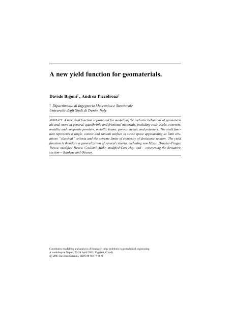
A new yield function for geomaterials. - Ingegneria - Università degli ...

A new yield function for geomaterials.
Davide Bigoni † , Andrea Piccolroaz †
† Dipartimento di Ingegneria Meccanica e Strutturale
Università degli Studi di Trento, Italy
ABSTRACT. A new yield function is proposed for modelling the inelastic behaviour of geomaterials
and, more in general, quasibrittle and frictional materials, including soils, rocks, concrete,
metallic and composite powders, metallic foams, porous metals, and polymers. The yield function
represents a single, convex and smooth surface in stress space approaching as limit situations
“classical” criteria and the extreme limits of convexity of deviatoric section. The yield
function is therefore a generalization of several criteria, including von Mises, Drucker-Prager,
Tresca, modified Tresca, Coulomb-Mohr, modified Cam-clay, and —concerning the deviatoric
section— Rankine and Ottosen.
Constitutive modelling and analysis of boundary value problems in geotechnical engineering
A workshop in Napoli, 22-24 April 2003, Viggiani, C. (ed)
c○ 2003 Hevelius Edizioni, ISBN 88-86977-36-0

266 Davide Bigoni, Andrea Piccolroaz
1. Introduction
Yielding or damage of quasibrittle and frictional materials (a collective denomination
for soil, concrete, rock, granular media, coal, cast iron, ice, porous metals,
metallic foams, as well as certain types of ceramic) is complicated by many effects,
including dependence on the first and third stress invariants (the so-called ‘pressuresensitivity’
and ‘Lode-dependence’ of yielding), and represents the subject of an intense
research effort. Restricting the attention to the formulation of yield criteria,
research moved in two directions: one was to develop such criteria on the basis of
micromechanics considerations, while another was to find direct interpolations to experimental
data. Examples of yield functions generated within the former approach
are numerous and, as a paradigmatic case, we may mention the celebrated Gurson
criterion (Gurson, 1977). The latter approach was also broadly followed, providing
some very successful yield condition, such as for instance the Ottosen criterion
for concrete (Ottosen, 1977). Although very fundamental in essence, the micromechanics
approach has however limits, particularly when employed for geomaterials.
For instance, it is usually based on variational formulations possible —for inelastic
materials— only for solids obeying the postulate of maximum dissipation at a microscale,
which is typically violated for frictional materials such as for instance soils.
A purely phenomenological point of view is assumed in the present article, where
a new yield function1 is formulated, tailored to interpolate experimental results for
quasibrittle and frictional materials, under the assumption of isotropy. The interest in
this proposal lies in the features evidenced by the criterion. These are:
– closure both in tension and in compression;
– non-circular deviatoric section of the yield surface, which may approach both
the upper and lower convexity limits for extreme values of material parameters;
– smoothness of the yield surface;
– extreme variation in shape of the yield surface and related capability of interpolating
a broad class of experimental data for different materials;
– reduction to known-criteria in limit situations;
– convexity of the yield function (and thus of the yield surface);
– simple mathematical expression.
None of the above features is essential, in the sense that a plasticity theory can be
developed without all of the above, but all are desirable for the development of certain
models of interest, particularly in the field of geomaterials.
1. We do not need to distinguish here between yield, damage and failure. Within a phenomenological
approach, all these situations are based on the concept of stress range, bounded by a
given hypersurface defined in stress space.

On a yield function 267
The range of material parameters corresponding to convexity of the proposed yield
function has been obtained by the autors in a related work (to appear), in which two
general propositions have been developed, that can be useful for analyzing convexity
of a broad class of yield functions. The propositions are shown to be constructive, in
the sense that these may be employed to generate convex yield functions.
2. Notation
The analysis will be restricted to isotropic behaviour, therefore the Haigh-Westergaard
representation of the yield locus is employed (Hill, 1950). This is well-known, so that
we limit the presentation here to a few remarks that may be useful in the following.
First, we recall that:
A1. a single point in the Haigh-Westergaard space is representative of the infinite (to
the power three) stress tensors having the same principal values;
A2. due to the arbitrary in the numeration of the eigenvalues of a tensor, six different
points correspond in the Haigh-Westergaard representation to a given stress
tensor. As a result, the yield surface results symmetric about the projections of
the principal axes on the deviatoric plane (Fig. 1);
A3. the Haigh-Westergaard representation preserves the scalar product only between
coaxial tensors;
A4. a convex yield surface —for a material with a fixed yield strength under triaxial
compression— must be internal to the two limit situations shown in Fig. 1
(Haythornthwaite, 1985). Note that the inner bound will be referred as ‘the
Rankine limit’.
Due to isotropy, the analysis of yielding can be pursued fixing once and for all a
reference system and restricting to all stress tensors diagonal in this system. We will
refer to this setting as to the Haigh-Westergaard representation. When tensors (for
instance, the yield function gradient) coaxial to the reference system are represented,
the scalar product is preserved, property A3. In the Haigh-Westergaard representation,
the hydrostatic and deviatoric stress components are defined by the invariants
tr σ
p = −
3 , q = 3J2, (1)
where
J2 = 1
tr σ
S · S, S = σ − I, (2)
2 3
in which S is the deviatoric stress, I is the identity tensor, a dot denotes scalar product
and tr denotes the trace operator, so that A · B = tr ABT , for every second-order

268 Davide Bigoni, Andrea Piccolroaz
2
1
3
Upper convexity
limit
Lower convexity
(Rankine) limit
Figure 1. Deviatoric section: definition of angle θ, symmetries, lower and upper convexity
bounds.
tensors A and B. The position of the stress point in the deviatoric plane is singled out
by the Lode (1926) angle θ defined as
θ = 1
3 cos−1
3 √ 3
2
J3
J2 3/2
, J3 = 1
3 tr S3 , (3)
so that θ ∈ [0,π/3]. As a consequence of property (A2) of the Haigh-Westergaard
representation, a single value of θ corresponds to six different points in the deviatoric
plane (Fig. 1). The following gradients of the invariants, that will be useful later,
∂p
∂σ
∂θ
∂σ
1 ∂J2 ∂J3
= − I, = S,
3 ∂σ
9
= −
2 q3 sin 3θ
S 2 −
∂σ = S2 −
tr S2
3 I,
tr S2 cos 3θ
I − q
3 3 S
can be obtained from well-known formulae (e.g. Truesdell and Noll, 1965, Sect. 9)
using the identity
∂S
∂σ
,
(4)
1
= I ⊗ I − I ⊗ I, (5)
3
where the symbol ⊗ denotes the usual dyadic product and I ⊗ I is the symmetrizing
fourth-order tensor, defined for every tensor A as I ⊗ I[A] =(A + A T )/2. Note that
∂θ/∂σ is orthogonal to I and to the deviatoric stress S.

On a yield function 269
3. A new yield function
We propose the seven-parameters yield function F : Sym → R ∪{+∞} defined
as:
F (σ) =f(p)+ q
,
g(θ)
(6)
where the dependence on the stress σ is included in the invariants p, q and θ, eqns (1)
and (3), through the ‘meridian’ function
⎧
⎨ −Mpc (Φ − Φm )[2(1−α)Φ + α]
f(p) =
⎩
+∞
if Φ ∈ [0, 1],
if Φ /∈ [0, 1],
(7)
where
p + c
Φ= ,
pc + c
(8)
describing the pressure-sensitivity and the ‘deviatoric’ function
g(θ) =
1
cos β π 1
6 − 3 cos−1 (γ cos 3θ)
, (9)
describing the Lode-dependence of yielding. The seven, non-negative material parameters:
M>0, pc > 0, c≥ 0, 0

270 Davide Bigoni, Andrea Piccolroaz
The yield function (6) corresponds to the following yield surface:
q = −f(p)g(θ), p ∈ [−c, pc], θ ∈ [0,π/3], (13)
which makes explicit the fact that f(p) and g(θ) define the shape of the meridian and
deviatoric sections, respectively.
The yield surface (13) is sketched in Figs. 2-3 for different values of the seven
above-defined material parameters (non-dimensionalization is introduced through division
by pc in Fig. 2). In particular, meridian sections are reported in Figs. 2, whereas
Fig. 3 pertains to deviatoric sections.
q/p c
q/p c
0.8
0.6
0.4
0.2
0
0.8
0.6
0.4
0.2
0
(a) 1.25
(b)
0.75
M=0.25
-0.4 -0.2 0 0.2 0.4 0.6 0.8 1 1.2 1.4
p/p c
(c) (d)
m=1.2
-0.4 -0.2 0 0.2 0.4 0.6 0.8 1 1.2 1.4
p/p c
2
4
q/p c
q/p c
0.8
0.6
0.4
0.2
0
0.8
0.6
0.4
0.2
0
0.4
0.2
c/p =0
C
-0.4 -0.2 0 0.2 0.4 0.6 0.8 1 1.2 1.4
p/p c
1.99
1
=0.01
-0.4 -0.2 0 0.2 0.4 0.6 0.8 1 1.2 1.4
p/p c
Figure 2. Meridian section: effects related to the variation of parameters M (a), c/pc (b), m
(c), and α (d).
As a reference, the case corresponding to the modified Cam-clay introduced by
Roscoe and Burland (1968) and Schofield and Wroth (1968) and corresponding to
β =1, γ =0, α =1, m = 2, and c = 0 is reported in Fig. 2 as a solid line,
for M = 0.75. The distortion of meridian section reported in Fig. 2(a) —where
M =0.25, 0.75, 1.25— can also be obtained within the framework of the modified
Cam-clay, whereas the effect of an increase in cohesion reported in Fig. 2(b) —where
c/pc =0, 0.2, 0.4— may be employed to model the gain in cohesion consequent to
plastic strain, during compaction of powders.
The shape distortion induced by the variation of parameters m and α, Fig. 2(c)
—where m =1.2, 2, 4— and 2(d) —where α =0.01, 1.00, 1.99— is crucial to fit
experimental results relative to frictional materials.

On a yield function 271
30
30
(a) = 0.99
(b) = 1
0
60
30
30
60
0
30
0 0.5 1 1.5 2
g( )
30
(c) = 0
(d) = 0.5
0
60
2.0
0
30
0.75
30
1.5
0.5
1.0
=0
=1
60
0
30
0 0.5
g( )
1
30
0
60
0
60
30
30
30
30
0
60
0
60
30
30
30
30
1.5
0.5
1.0
=0
60
0
30
0 0.5 1 1.5 2
g( )
60
0
30
30
0 0.5
g( )
1
Figure 3. Deviatoric section: effects related to the variation of β and γ. Variation of β =
0, 0.5, 1, 1.5, 2 at fixed γ =0.99 (a) and γ =1(b). Variation of γ =1, 0.75, 0 at fixed β =0
(c) and β =0.5 (d).
The possibility of extreme shape distortion of the deviatoric section, which may
range between the upper and lower convexity limits, and approach Tresca, von Mises
and Coulomb-Mohr, is sketched in Fig. 3. It should be noted that to simplify reading
of the figure, function g(θ) has been normalized through division by g(π/3), so that
all deviatoric sections coincide at the point θ = π/3. Parameter γ is kept fixed in
Figs. 3 (a) and (b) and equal to 0.99 and 1, respectively, whereas parameter β is fixed
in Figs. 3 (c) and (d) and equal to 0 and 1/2. Therefore, figures (a) and (b) demonstrate
the effect of the variation in β (= 0, 0.5, 1, 1.5, 2) which makes possible a distortion
of the yield surface from the upper to lower convexity limits going through Tresca
and Coulomb-Mohr shapes. The role played by γ (= 1, 0.75, 0) is investigated in
figures (c) and (d), from which it becomes evident that γ has a smoothing effect on
the corners, emerging in the limit γ =1. The von Mises (circular) deviatoric section
emerges when γ =0.
The yield surface in the biaxial plane σ1 versus σ2, with σ3 =0is sketched in
Fig. 4, where axes are normalized through division by the uniaxial tensile strength f t.
0
2.0
0.75
=1
30
0
60
0
60
30
30

272 Davide Bigoni, Andrea Piccolroaz
In particular, the figure pertains to M =0.75, pc =50c, m =2, and α =1, whereas
γ =0.99 is fixed and β is equal to {0, 0.5, 1, 1.5, 2} in Fig. 4(a) and, vice-versa,
β =0is fixed and γ is equal to {0, 0.75, 0.99} in Fig. 4(b).
=0
(a) = 0.99
(b) = 0
0.5
- 12 - 10 - 8 - 6 - 4 - 2
2
1.5
1
/f t
- 2
- 4
- 6
- 8
- 10
- 12
1 /f t
=0.99
- 12 - 10 - 8 - 6 - 4 - 2
Figure 4. Yield surface in the biaxial plane σ1/ft vs. σ2/ft, with σ3 = 0. Variation of
β =0, 0.5, 1, 1.5, 2 at fixed γ =0.99 (a) and variation of γ =0, 0.75, 0.99 at fixed β =0(b).
3.1. Reduction of yield criterion to known cases
The yield function (6)-(9) reduces to almost all 2 ‘classical’ criteria of yielding.
These can be obtained as limit cases in the way illustrated in Tab. 1 where the modified
Tresca criterion was introduced by Drucker (1953), whereas the Haigh-Westergaard
representation of the Coulomb-Mohr criterion was proposed by Shield (1955). In
Tab. 1 parameter r denotes the ratio between the uniaxial strengths in compression
(taken positive) and tension, indicated by f c and ft, respectively. We note that for real
materials r ≥ 1 and that we did not explicitly consider the special cases of no-tension
ft =0or granular ft = fc =0materials [which anyway can be easily incorporated
as limits of (6)-(9)].
We note that the expression of the Tresca criterion which follows from (6)-(9) in
the limits specified in Tab. 1, was provided also by Bardet (1990) and answers —
in a positive way— the question (raised by Salençon, 1974) if a proper form of the
criterion in terms of stress invariants exist.
2. A remarkable exception is the isotropic Hill (1950 b) criterion, corresponding to a Tresca
criterion rotated of π/6 in the deviatoric plane.
0.75
0
- 10
- 12
/f t
- 2
- 4
- 6
- 8
1 /f t

On a yield function 273
Table 1. Yield criteria obtained as special cases of (6)-(9), r = fc/ft and fc and ft are the
uniaxial strengths in compression and tension, respectively.
Criterion Meridian function f(p) Deviatoric function g(θ)
von Mises
Drucker-Prager
Tresca
mod. Tresca
Coulomb-Mohr
α =1, m =2,
M = 2ft
, c = pc −→ ∞
pc
α =0, M =
3(r − 1)
√ 2(r +1) ,
c = 2fc
, pc = fc m −→ ∞
3(r − 1)
as for von Mises,
√
except that
3ft
M =
pc
as for Drucker-Prager, except that
M = 3√3(r − 1)
2 √ 2(r +1)
as for Drucker-Prager, except that
M = 3 r cos β π
π
π
− − cos β 6 3
6
√
2(r +1)
c = fc
π π
π
cos β − +cosβ 6 3
6
π
− 3cosβ
3r cos β π
6
− π
3
6
β =1, γ =0
as for von Mises
β =1, γ −→ 1
as for Tresca
β = 6
π tan−1
√
3
2r +1 ,
γ −→ 1
mod. Cam-clay m =2,α=1,c=0 as for von Mises
The Mohr-Coulomb limit merits a special mention. In fact, if the following values
of the parameters are selected
α =0, c = fc
π π
π
cos β 6 − 3 +cosβ6 3r cos β π
π
π ,
6 − 3 − 3cosβ6 M = 3 r cos β π
(14)
π
π
6 − 3 − cos β 6
√ ,
2(r +1)

274 Davide Bigoni, Andrea Piccolroaz
and then the limits
γ −→ 1, pc = fc m −→ ∞, (15)
are performed, a three-parameters generalization of Coulomb-Mohr criterion is obtained,
which reduces to the latter criterion in the special case when β is selected in
the form specified in Tab. 1 (yielding an expression noted also by Chen and Saleeb,
1982). The cases reported in Tab. 1 refer to situations in which the criterion (6)-(9)
reduces to known yield criteria both in terms of function f(p) and of function g(θ).
It is however important to mention that the Lode’s dependence function g(θ) reduces
also to well-known cases, but in which the pressure-sensitivity cannot be described by
the meridian function (7). These are reported in Tab. 2. It is important to mention that
the form of our function g(θ), eqn. (9), was indeed constructed as a generalization of
the deviatoric function introduced by Ottosen (1977).
Table 2. Deviatoric yield functions obtained as special cases of (9)
Criterion Deviatoric function g(θ)
Lower convexity (Rankine) β =0, γ −→ 1
Upper convexity β =2, γ −→ 1
Ottosen β =0, 0 ≤ γ

On a yield function 275
q (MPa)
0.8
0.6
0.4
0.2
0.2
0.4
(a) (b)
0.2 0.4 0.6 0.8 1
=
=
p (MPa)
q/p e
0.6
0.4
0.2
- 0.2
- 0.4
0.2 0.4 0.6 0.8 1
p/p e
=0 =0
Figure 5. Comparison with experimental results relative to sand (Yasufuku et al. 1991) (a)
and clay (Parry, reported by Wood, 1990) (b).
and Fleck (2000) —their Figs. 5(b) and 9(c)— relative to ductile powders is reported
in Fig. 6. In particular, Fig. 6(a) is relative to an aluminum powder (Al D 0=0.67,
D=0.81 in Sridhar and Fleck, their Fig. 5b), Fig. 6(b) to an aluminum powder reinforced
by 40 vol.%SiC (Al-40%Sic D0=0.66, D=0.82 in Sridhar and Fleck, their
Fig. 5b), Fig. 6(c) to a lead powder (0% steel in Sridhar and Fleck, their Fig. 9c), and
Fig. 6(d) to a lead shot-steel composite powder (20% steel in Sridhar and Fleck, their
Fig. 9c). Beside the fairly good agreement between experiments and proposed yield
function, we note that the aluminium powder has a behaviour —different from soils
and lead-based powders— resulting in a meridian section of the yield surface similar
to the early version of the Cam-clay model (Roscoe and Schofield, 1963).
Regarding concrete, among the many experimental results currently available, we
have referred to Sfer et al. (2002, their Fig. 6) and to the Newman and Newman (1971)
empirical relationship
σ1
fc
=1+3.7
σ3
fc
0.86
, (16)
where σ1 and σ3 are the maximum and minimum principal stresses at failure and f c
is the value of the ultimate uniaxial compressive strength. Small circles in Fig. 7 represents
results obtained using relationship (16) in figure (a) and experimental results
by Sfer et al. (2002) in figure (b); the approximation provided by the criterion (7)-(8)
is also reported as a continuous line.
As far as rocks are concerned, we limit to a few examples. However, we believe
that due to the fact that our criterion approaches Coulomb-Mohr, it should be particularly
suited for these materials. In particular, data taken from Hoek and Brown (1980,
their pages 143 and 144) are reported in Fig. 8 as small circles for two rocks, chert
(Fig. 8a) and dolomite (Fig. 8b).
A few data on polymers are reported in Fig. 9 —together with the fitting provided
by our model— concerning polymethil methacrylate (Fig. 9a) and an epoxy binder

276 Davide Bigoni, Andrea Piccolroaz
q/p C
q/p C
0.8
0.7
0.6
0.5
0.4
0.3
0.2
0.1
0.5
0.4
0.3
0.2
0.1
(a) (b)
=
=
0.2 0.4 0.6 0.8 1
p/p C
p/p C
q/p C
q/p C
0.5
0.4
0.3
0.2
0.1
0.2 0.4 0.6 0.8 1
p/p C
(c) (d)
=
=
0.2 0.4 0.6 0.8 1
0.5
0.4
0.3
0.2
0.1
0.2 0.4 0.6 0.8 1
Figure 6. Comparison with experimental results relative to aluminium powder (a) aluminum
composite powder (b), lead powder (c) and lead shot-steel composite powder(d), data taken
from Sridhar and Fleck (2000).
q/f C
30
25
20
15
10
5
p/f C
q/f C
p/p C
(a) =
(b) =
5 10 15 20 25 30
5
4
3
2
1
- 1 1 2 3 4
Figure 7. Comparison with the experimental relation (16) proposed by Newman and Newman
(1971) (a) and with results by Sfer et al. (2002) (b).
(Fig. 9b), taken from Ol’khovik (1983, their Fig. 5), see also Altenbach and Tushtev
(2001, their Figs. 2 and 3).
Finally, our model describes —with a different yield function— the same yield
surface proposed by Deshpande and Fleck (2000) to describe the behaviour of metallic
foams. In particular, the correspondence between parameters of our model (6)-(9) and
p/f C

On a yield function 277
q/f C
4
3.5
3
2.5
2
1.5
1
0.5
(a) =
(b) =
0.5 1 1.5 2
p/f C
q/f C
4
3.5
3
2.5
2
1.5
1
0.5
0.5 1 1.5 2
Figure 8. Comparison with experiments for rocks. Chert (a) and dolomite (b), data taken from
Hoek and Brown (1980).
q (MPa)
250
200
150
100
50
p (MPa)
q (MPa)
p/f C
(a) =
(b) =
100 200 300 400
250
200
150
100
50
100 200 300 400
p (MPa)
Figure 9. Comparison with experimental results for polymers. Methacrylate (a) and an epoxy
binder (b), data taken from Ol’khovik (1983).
of the yield surface proposed by Deshpande and Fleck [2000, their eqns. (2)-(3)] is
obtained setting
β =1, γ =0, m =2, α =1,
and assuming the correlations given in Tab. 3.
The proposed function (6)-(9) is also expected to model correctly yielding of
porous ductile metals. As a demonstration of this, we present in Fig. 10 a comparison
with the Gurson (1977) model. The Gurson yield function has a circular deviatoric
section so that β =1and γ =0in our model, in addition, we select
α =1, m =2,
2
pc = c = σM
3q2
2
M = σM 1+q3f 2 − 2fq1,
pc
cosh −1 1+q3f 2
2fq1
,
(17)

278 Davide Bigoni, Andrea Piccolroaz
Table 3. Correspondence between parameters of (6)-(9) and Deshpande and Fleck (2002) yield
functions —the latter shortened as ‘DF model’— to describe the behaviour of metallic foams.
DF model
Y ,α 2α
Model (6)-(9) DF model
M c pc Y α
Y
1+
α
α
2 Y
1+
3 α
Model (6)-(9)
M,pc,c — — —
α
2 3
2
— —
cM
1+ M
6
where f is the void volume fraction (taking the values {0.01, 0.1, 0.3, 0.6 } in Fig. 10),
σM is the equivalent flow stress in the matrix material and q1 =1.5, q2 =1and
q3 = q 2 1 are the parameters introduced by Tvergaard (1981, 1982). A good agreement
between the two models can be appreciated from Fig. 10, increasing when the void
volume fraction f increases.
q/ M
1
0.8
0.6
0.4
0.2
0.6
0.3
0.1
0.5 1 1.5 2 2.5 3 3.5
p/
Present model
Gurson model
f = 0.01
Figure 10. Comparison with the Gurson model at different values of void volume fraction f.
As far as the deviatoric section is regarded, we limit to two examples —reported
in Fig. 11— concerning sandstone and dense sand, where the experimental data have
been taken from Lade (1997, their Figs. 2 and 9a).
Experimental data referred to the biaxial plane σ 3 =0for grey cast iron and concrete
(taken respectively from Coffin and Schenectady, 1950, their Fig. 5 and Tasuji et
al. 1978, their Figs. 1 and 2) are reported in Fig. 12.
2
M
2

On a yield function 279
30
(a)
(b)
0
60
30
30
60
0
30
30
0
0 0.5
g( )
1
60
30
30
0
60
30
30
60
0
30
30
0
0 0.5
g( )
1
Figure 11. Comparison with experimental results relative to deviatoric section for sandstone
(a) and dense sand (b) data taken from (Lade, 1997).
(a) (b)
0.5
- 1.5 - 1 - 0.5 0.5
- 0.5
- 1
- 1.5
/f C
1 /fC
- 1.5 - 1 - 0.5 0.5
Figure 12. Comparison with experimental results on biaxial plane for cast iron (data taken
from Coffin and Schenectady, 1950)(a) and concrete (data taken from Tasuji et al. 1978)(b).
4. Conclusions
In the modelling of the inelastic behaviour of several materials, the knowledge of
a smooth yield surface approaching know-criteria and possessing an extreme shape
variation to fit experimental results may be very useful. In the present paper, such
a yield function has been proposed, which is shown to be capable of an accurate description
of the behaviour of a broad class of materials including soils, concrete, rocks,
powders, metallic foams, porous materials, and polymers.
References
Altenbach, H., Tushtev, K., 2001, A new static failure criterion for isotropic polymers, Mech.
Compos. Mater., 37, 475-482.
Bardet, J.P., 1990, Lode dependences for isotropic pressure-sensitive elastoplastic materials, J.
Appl. Mech., 57, 498-506.
0.5
- 0.5
- 1
- 1.5
/f C
60
30
1 /fC

280 Davide Bigoni, Andrea Piccolroaz
Chen, W.F., Saleeb, A.F., 1982, Constitutive equations for engineering materials: elasticity and
modelling, Wiley & Sons, New York.
Coffin, L.F., Schenectady, N.Y., 1950, The flow and fracture of a brittle material, J. Appl. Mech.,
17, 233-248.
Deshpande, V.S., Fleck, N.A., 2000, Isotropic constitutive models for metallic foams, J. Mech.
Phys. Solids, 48, 1253-1283.
Drucker, D.C., 1953, Limit analysis of two and three dimensional soil mechanics problems, J.
Mech. Phys. Solids, 1, 217-226.
Gurson, A.L., 1977, Continuum theory of ductile rupture by void nucleation and growth: part
I, yield criteria and flow rules for porous ductile media, Int. J. Engng. Mat. Tech., 99, 2-15.
Haythornthwaite, R.M., 1985, A family of smooth yield surfaces, Mechanics Research Communications,
12, 87-91.
Hill, R., 1950 a, The mathematical theory of plasticity, Clarendon Press, Oxford.
Hill, R., 1950 b, Inhomogeneous deformation of a plastic lamina in a compression test, Phil.
Mag., 41, 733-744.
Hoek, E., Brown, E.T., 1980, Underground excavations in rock, The Institution of Mining and
Metallurgy, London.
Lade P.V., 1997, Modelling the strengths of engineering materials in three dimensions, Mech.
Cohes. Frict. Mat., 2, 339-356.
Lode, W., 1926, Versuche über den Einfluß der mittleren Hauptspannung auf das Fließen der
Metalle Eisen Kupfer und Nickel, Z. Physik., 36, 913-939.
Newman, K., Newman, J.B., 1971, Failure theories and design criteria for plain concrete, in:
Structure, Solid Mechanics and Engineering Design, Proc. 1969 Southampton Civil Engineering
Conf., Te’eni, M. Ed., Wiley Interscience, New York, pp. 963-995.
Ol’khovik, O., 1983, Apparatus for testing of strength of polymers in a three-dimensional
stressed state, Mech. Compos. Mater., 19, 270-275.
Ottosen, N.S., 1977, A failure criterion for concrete, J. Eng. Mech. Div.-ASCE, 103, 527-535.
Roscoe, K.H., Burland, J.B., 1968, On the generalized stress-strain behaviour of ’wet’ clay, Engineering
Plasticity, Heyman, J. and Leckie, F.A., Eds., Cambridge University Press, Cambridge.
Roscoe, K.H., Schofield, A.N., 1963, Mechanical behaviour of an idealised ’wet’ clay, Proc. European
Conf. on Soil Mechanics and Foundation Engineering, Wiesbaden (Essen: Deutsche
Gesellshaft für Erd- und Grundbau e. V.), vol. 1, pp. 47-54.
Salençon, J., 1974, Applications of the theory of plasticity in soil mechanics, Wiley & Sons,
Chichester.
Schofield, A.N., Wroth, C.P., 1968, Critical state soil mechanics, McGraw-Hill Book Company,
London.
Sfer, D., Carol, I., Gettu, R., Etse, G., 2002, Study of the behaviour of concrete under triaxial
compression, ASCE J. Engng. Mech., 128, 156-163.
Shield, R.T., 1955, On Coulomb’s law of failure in soils, J. Mech. Phys. Solids, 4, 10-16.
Sridhar, I., Fleck, N.A., 2000, Yield behaviour of cold compacted composite powders, Acta
mater., 48, 3341-3352.
Tasuji, M.E., Slate, F.O., Nilson, A.H., 1978, Stress-strain response and fracture of concrete in
biaxial loading, ACI J., 75, 306-312.
Truesdell, C. and Noll, W., 1965, The non-linear field theories of mechanics, in Flügge, S., ed.,
Encyclopedia of Physics:III/3, Springer-Verlag, Berlin.
Tvergaard, V., 1981, Influence of voids on shear band instabilities under plane strain conditions,
Int. J. Fracture, 17, 389-407.

On a yield function 281
Tvergaard, V., 1982, On localization in ductile materials containing spherical voids, Int. J. Fracture,
18, 237-252.
Wood, D.M., 1990, Soil behaviour and critical state soil mechanics, Cambridge University
Press, Cambridge.
Yasufuku, N., Murata, H., Hyodo, M., 1991, Yield characteristics of anisotropically consolidated
sand under low and high stress, Soils and Foundations, 31, 95-109.