journal of forest science

That means they are the recursive system of equations
from the equation structure point of view. orest biometricians
usually work with models which have recursive
relation in nature (sequential relationships between some
equations) but which also exhibit cross-equation correlation
between error com- ponents. The endogenous variable
H2 in equation (3) is not a function of other
endogenous variables, but the endogenous variable G2
in equation (2) is a function of H2 in equation (3), and
the endogenous variable V2 in equation (1) is a function
of H2 in equation (3) and G2 in equation (2). Application
of OLS method to each of the structural equations
leads to unbiased, consistent, and asymptotically efficient
parameter estimates if the variance-covariance matrix of
the structural errors for the recursive system of equations
is diagonal. The RHS endogenous variables will be correlated
with the error components of the LHS endogenous
variables if significant cross-equations are present
and the system is not recursive by definition (BORDERS
1989). urthermore, the consistent estimators will not be
produced by implementing OLS. However, nonlinear
3SLS and SUR could be used to estimate parameters
(BORDERS 1989).
COMPARISON O ALTERNATIVE METHODS O
ESTIMATION
The methods of estimating structural equations of
a general interdependent system, especially recursive system
of equations, have been discussed. Therefore, it
might be of interest to compare the results obtained from
the system of equations (1) and (3) by the different estimation
methods, which are nonlinear ordinary least
squares (NOLS) and nonlinear three-stage least squares
(N3SLS) and nonlinear seemingly unrelated regression
(NSUR). The results from NOLS are shown and compared
to N3SLS and NSUR because NOLS is commonly
used in applied work. In this case comparing various estimators
is like comparing different guns on the basis of
one shot from each. All estimates are accomplished by
using TSP 386 program (TSP International 1990). The
Gauss-Newton iterative method using the Taylor series
expansion as described in AMEMIYA (1988) was applied
to all fits because an advantage of the Gauss-Newton iterative
method over the Newton-Raphson iteration is that
the former requires only the first derivatives of expanding
function.
The criteria of comparison in different methods of estimation
are calculated for each equation according to
the following indicators.
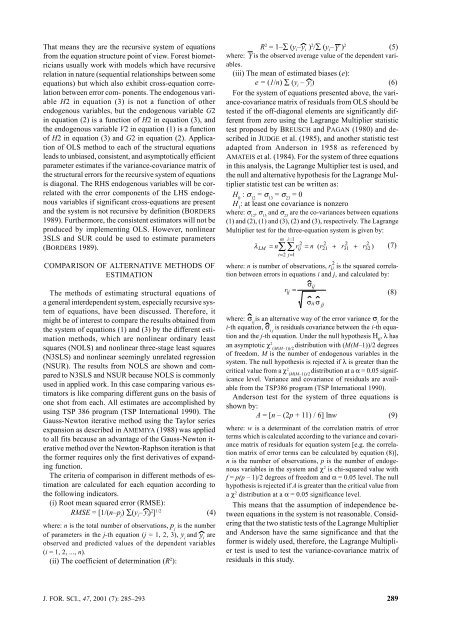
(i) Root mean squared error (RMSE):
RMSE = [1/(n–pj) ∑(yi– ) 2 ] 1/2 (4)
where: n is the total number of observations, p is the number
j
of parameters in the j-th equation (j = 1, 2, 3), y and are
i yi observed and predicted values of the dependent variables
(i = 1, 2, ..., n).
(ii) The coefficient of determination (R 2 ):
y i
R
where: Y is the observed average value of the dependent variables.
(iii) The mean of estimated biases (e):
e = (1/n) ∑ (yi – yi) (6)
or the system of equations presented above, the variance-covariance
matrix of residuals from OLS should be
tested if the off-diagonal elements are significantly different
from zero using the Lagrange Multiplier statistic
test proposed by BREUSCH and PAGAN (1980) and described
in JUDGE et al. (1985), and another statistic test
adapted from Anderson in 1958 as referenced by
AMATEIS et al. (1984). or the system of three equations
in this analysis, the Lagrange Multiplier test is used, and
the null and alternative hypothesis for the Lagrange Multiplier
statistic test can be written as:
H : σ = σ = σ = 0
0 12 13 23
H : at least one covariance is nonzero
1
where: σ , σ and σ are the co-variances between equations
12 13 23
(1) and (2), (1) and (3), (2) and (3), respectively. The Lagrange
Multiplier test for the three-equation system is given by:
2 = 1–∑ (yi– ) 2 /∑ (yi– ) 2 yi Y
(5)
2
where: n is number of observations, ri
j
is the squared correlation
between errors in equations i and j, and calculated by:
rij
=
σij
σii
σ jj
(8)
where: is an alternative way of the error variance σ for the i
i-th equation, is residuals covariance between the i-th equation
and the j-th equation. Under the null hypothesis H , λ has 0
an asymptotic χ2 distribution with (M(M–1))/2 degrees
(M(M–1))/2
of freedom. M is the number of endogenous variables in the
system. The null hypothesis is rejected if λ is greater than the
critical value from a χ2 σi j
distribution at a α = 0.05 signif-
(M(M–1))/2
icance level. Variance and covariance of residuals are available
from the TSP386 program (TSP International 1990).
Anderson test for the system of three equations is
shown by:
A = [n – (2p + 11) / 6] lnw (9)
where: w is a determinant of the correlation matrix of error
terms which is calculated according to the variance and covariance
matrix of residuals for equation system [e.g. the correlation
matrix of error terms can be calculated by equation (8)],
n is the number of observations, p is the number of endogenous
variables in the system and χ 2 is chi-squared value with
f = p(p – 1)/2 degrees of freedom and α = 0.05 level. The null
hypothesis is rejected if A is greater than the critical value from
a χ 2 distribution at a α = 0.05 significance level.
This means that the assumption of independence between
equations in the system is not reasonable. Considering
that the two statistic tests of the Lagrange Multiplier
and Anderson have the same significance and that the
former is widely used, therefore, the Lagrange Multiplier
test is used to test the variance-covariance matrix of
residuals in this study.
J. FOR. SCI., 47, 2001 (7): 285–293 289
σ ii
λ
LM
= n
m i=
1
2
∑∑rij
i=
2 j=
1
= n ( r
2
21
+
2
31
r
+
2
32
r
)
(7)