Using the Pareto Distribution in Queueing Modeling - Classweb ...
Using the Pareto Distribution in Queueing Modeling - Classweb ...
Using the Pareto Distribution in Queueing Modeling - Classweb ...

You also want an ePaper? Increase the reach of your titles
YUMPU automatically turns print PDFs into web optimized ePapers that Google loves.
Abstract<br />
Submitted to Journal of Probability and Statistical Science, Mar. 2005.<br />
<strong>Us<strong>in</strong>g</strong> <strong>the</strong> <strong>Pareto</strong> <strong>Distribution</strong> <strong>in</strong> Queue<strong>in</strong>g Model<strong>in</strong>g<br />
John Shortle Mart<strong>in</strong> Fischer<br />
Donald Gross Denise Masi<br />
George Mason University Mitretek Systems<br />
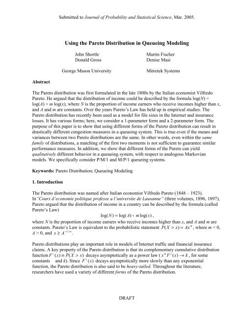
The <strong>Pareto</strong> distribution was first formulated <strong>in</strong> <strong>the</strong> late 1800s by <strong>the</strong> Italian economist Vilfredo<br />
<strong>Pareto</strong>. He argued that <strong>the</strong> distribution of <strong>in</strong>come could be described by <strong>the</strong> formula log(N) =<br />
log(A) + m log(x), where N is <strong>the</strong> proportion of <strong>in</strong>come earners who receive <strong>in</strong>comes higher than x,<br />
and A and m are constants. Over <strong>the</strong> years <strong>Pareto</strong>’s Law has held up <strong>in</strong> empirical studies. The<br />
<strong>Pareto</strong> distribution has recently been used as a model for file sizes <strong>in</strong> <strong>the</strong> Internet and <strong>in</strong>surance<br />
losses. It has various forms; here, we consider a 1-parameter form and a 2-parameter form. The<br />
purpose of this paper is to show that us<strong>in</strong>g different forms of <strong>the</strong> <strong>Pareto</strong> distribution can result <strong>in</strong><br />
drastically different congestion measures <strong>in</strong> a queue<strong>in</strong>g system. This is true even if <strong>the</strong> means and<br />
variances between two <strong>Pareto</strong> distributions are <strong>the</strong> same. In o<strong>the</strong>r words, even with<strong>in</strong> <strong>the</strong> same<br />
family of distributions, a match<strong>in</strong>g of <strong>the</strong> first two moments is not sufficient to guarantee similar<br />
performance measures. In addition, we show that different forms of <strong>the</strong> <strong>Pareto</strong> can yield<br />
qualitatively different behavior <strong>in</strong> a queue<strong>in</strong>g system, with respect to analogous Markovian<br />
models. We specifically consider P/M/1 and M/P/1 queue<strong>in</strong>g systems.<br />
Keywords: <strong>Pareto</strong> <strong>Distribution</strong>; Queue<strong>in</strong>g Model<strong>in</strong>g<br />
1. Introduction<br />
The <strong>Pareto</strong> distribution was named after Italian economist Vilfredo <strong>Pareto</strong> (1848 – 1923).<br />
In“Cours d’economie politique professe a l’universite de Lausanne” (three volumes, 1896, 1897),<br />
<strong>Pareto</strong> argued that <strong>the</strong> distribution of <strong>in</strong>come <strong>in</strong> a country can be described by <strong>the</strong> formula (called<br />
<strong>Pareto</strong>’s Law)<br />
log( N ) = log( A)<br />
+ m log( x)<br />
,<br />
where N is <strong>the</strong> proportion of <strong>in</strong>come earners who receive <strong>in</strong>comes higher than x, and A and m are<br />
m<br />
constants. <strong>Pareto</strong>’s Law is equivalent to <strong>the</strong> probabilistic statement P ( X > x)<br />
= Ax , where m < 0,<br />
−1/<br />
m<br />
A > 0, and x ≥ A .<br />
<strong>Pareto</strong> distributions play an important role <strong>in</strong> models of Internet traffic and f<strong>in</strong>ancial <strong>in</strong>surance<br />
claims. A key property of <strong>the</strong> <strong>Pareto</strong> distribution is that its complementary cumulative distribution<br />
function F ( x)<br />
P(<br />
X x)<br />
decays asymptotically as a power law ( , for some<br />
constants and k). S<strong>in</strong>ce decays asymptotically more slowly than any exponential<br />
function, <strong>the</strong> <strong>Pareto</strong> distribution is also said to be heavy-tailed. Throughout <strong>the</strong> literature,<br />
researchers have used a variety of different forms of <strong>the</strong> <strong>Pareto</strong> distribution.<br />
c<br />
α c<br />
≡ ><br />
x F ( x)<br />
→ k<br />
F (x)<br />
c<br />
DRAFT
The purpose of this paper is to show that us<strong>in</strong>g different forms of <strong>the</strong> <strong>Pareto</strong> distribution can result<br />
<strong>in</strong> drastically different performance measures <strong>in</strong> a queue<strong>in</strong>g system. This is true even if <strong>the</strong> means<br />
and variances between two <strong>Pareto</strong> distributions are <strong>the</strong> same. Previous research has compared <strong>the</strong><br />
impact of us<strong>in</strong>g different families of heavy-tailed distributions – specifically <strong>the</strong> Weibull, <strong>Pareto</strong>,<br />
and lognormal distributions – <strong>in</strong> M/G/1, G/M/1, and G/M/c/c queues [5], [6], [14]. In this paper,<br />
we show that qualitatively different performance measures can result from us<strong>in</strong>g different<br />
distributions with<strong>in</strong> <strong>the</strong> same <strong>Pareto</strong> family of distributions – even when <strong>the</strong> first two moments are<br />
matched.<br />
Table 1 summarizes various forms of <strong>the</strong> <strong>Pareto</strong> distribution that have been used by researchers.<br />
α c<br />
All forms follow an asymptotic power law with shape parameter ( x F ( x)<br />
→ k ). Form (2c)<br />
seems to be used most widely <strong>in</strong> <strong>the</strong> literature. Many textbooks use this form (e.g., [13]), as does<br />
<strong>the</strong> popular distribution fitt<strong>in</strong>g package, ExpertFit. This form is used <strong>in</strong> many papers deal<strong>in</strong>g with<br />
Internet traffic (e.g., [4], [7], [15]) and <strong>in</strong>surance claims (e.g., [1], [11]). This form also directly fits<br />
α<br />
<strong>Pareto</strong>’s law given above, with γ and<br />
−<br />
A = m = −α<br />
.<br />
Form (3) <strong>in</strong> <strong>the</strong> table is <strong>the</strong> most general, <strong>in</strong>volv<strong>in</strong>g three parameters – shape , scale , and<br />
location (or shift). The o<strong>the</strong>r forms can be obta<strong>in</strong>ed from (3) by sett<strong>in</strong>g appropriate values for<br />
and/or , as shown <strong>in</strong> <strong>the</strong> table. In our previous work, (e.g., see [9], [10], [16], [17]), we have used<br />
form (1) due to its simplicity and because it allows <strong>the</strong> random variable to start at zero, <strong>in</strong>stead of a<br />
m<strong>in</strong>imum threshold.<br />
Number of<br />
Parameters<br />
Table 1. Forms of <strong>the</strong> <strong>Pareto</strong> <strong>Distribution</strong><br />
Reference<br />
Number Parameter Restrictions F ( t)<br />
1 F(<br />
t)<br />
c<br />
= −<br />
3 (3) α, β > 0, γ ≥ 0<br />
2<br />
(2a) Set γ = 0<br />
(2b) Set β =1<br />
(2c) Set β = γ<br />
1 (1) Set γ = 0, β =1<br />
⎛ β ⎞<br />
⎜ ⎟<br />
⎝t<br />
+ β − γ ⎠<br />
⎛ β ⎞<br />
⎜ ⎟⎠<br />
⎝t<br />
+ β<br />
α<br />
γ ⎟ ⎛ 1 ⎞<br />
⎜<br />
⎝t<br />
+1 − ⎠<br />
⎛γ<br />
⎞<br />
⎜ ⎟⎠<br />
⎝ t<br />
α<br />
⎛ 1 ⎞<br />
⎜ ⎟<br />
⎝t<br />
+1⎠<br />
α<br />
α<br />
α<br />
(t ≥ γ ≥ 0)<br />
(t ≥ 0)<br />
(t ≥ γ ≥ 0)<br />
(t ≥ γ > 0)<br />
(t ≥ 0)<br />
A key issue is that several forms of <strong>the</strong> <strong>Pareto</strong> distribution (and <strong>in</strong> particular, form (2c)) have a<br />
m<strong>in</strong>imum value strictly greater than zero. In o<strong>the</strong>r words, <strong>the</strong> random variable cannot take on<br />
values between zero and some value > 0. In a queue<strong>in</strong>g system, this could imply, for example, a<br />
m<strong>in</strong>imum time between successive arrivals, or a m<strong>in</strong>imum service time. We show that this has<br />
important consequences on performance measures of a queue<strong>in</strong>g system. Thus, care should be<br />
taken when us<strong>in</strong>g <strong>the</strong>se forms.<br />
2
In this paper, we <strong>in</strong>vestigate how <strong>the</strong> form of <strong>the</strong> <strong>Pareto</strong> <strong>in</strong>fluences congestion measures of a<br />
queue<strong>in</strong>g model. We specifically consider <strong>the</strong> P/M/1 and M/P/1 queues (where P stands for<br />
<strong>Pareto</strong>).<br />
2. The <strong>Pareto</strong> <strong>Distribution</strong>s Compared <strong>in</strong> this Study<br />
In this paper, we compare two forms of <strong>the</strong> <strong>Pareto</strong> distribution: <strong>the</strong> popular (2c) form and <strong>the</strong><br />
s<strong>in</strong>gle parameter (1) form. The o<strong>the</strong>r forms reduce ei<strong>the</strong>r to form (1) or (2c) when match<strong>in</strong>g<br />
moments or shape parameters, as discussed <strong>in</strong> <strong>the</strong> next paragraph, so it suffices just to compare<br />
<strong>the</strong>se forms. The key difference is that form (2c) has a m<strong>in</strong>imum value of , while form (1) has a<br />
m<strong>in</strong>imum value of 0. Table 2 gives <strong>the</strong> means and variances of both distributions, and also gives<br />
necessary and sufficient conditions for <strong>the</strong> first two moments to exist. (In general, for <strong>the</strong> k th<br />
moment to exist, <strong>the</strong> shape parameter must be greater than k.)<br />
Form<br />
(1)<br />
(2c)<br />
F (x)<br />
c<br />
⎛ 1 ⎞<br />
⎜ ⎟<br />
⎝t<br />
+1⎠<br />
⎛γ<br />
⎞<br />
⎜ ⎟⎠<br />
⎝ t<br />
α<br />
2<br />
Table 2. Comparison of moments of <strong>Pareto</strong> distributions<br />
α<br />
Mean Variance<br />
1<br />
α − 1<br />
α 2γ<br />
α − 1<br />
2<br />
2<br />
1<br />
−<br />
( α − 2)(<br />
α − 1)<br />
( α − 1<br />
2<br />
α 2γ<br />
⎛ α ⎞ 2γ<br />
− ⎜ ⎟<br />
α − 2 ⎝ α − 1⎠<br />
2<br />
2<br />
2<br />
2<br />
)<br />
Conditions for Existence of<br />
First Two Moments<br />
t > 0, α > 2<br />
t > γ, α2 > 2<br />
We specifically look at two different ways of match<strong>in</strong>g distributions:<br />
Case I: Match <strong>the</strong> mean and variance,<br />
Case II: Match <strong>the</strong> mean and shape parameter<br />
In Case I, <strong>the</strong> coefficients of variation (CV = <strong>the</strong> standard deviation divided by <strong>the</strong> mean) are<br />
equal, but <strong>the</strong> asymptotic tail behavior is different. For Case II, <strong>the</strong> tail behavior is similar (i.e., a<br />
similar asymptotic power law), but <strong>the</strong> variances are not equal. The relationships between<br />
parameters that achieve <strong>the</strong> appropriate matches are:<br />
α 2 −1<br />
Case I: α 2 = 1+<br />
2 − 2 / α , γ =<br />
(assum<strong>in</strong>g > 2 and 2 > 2),<br />
α ( α −1)<br />
Case II: α = α<br />
2 , γ<br />
2<br />
1/<br />
α<br />
= (assum<strong>in</strong>g > 1 and 2 > 1).<br />
For Case I, 2 is monotonically <strong>in</strong>creas<strong>in</strong>g as a function of , start<strong>in</strong>g at 2 and bounded above by<br />
1+ 2 . In addition, we can show that 2 when Thus, for Case I, we have 2<br />
and also 1+ 2 > 2 > 2. This implies that <strong>the</strong> 1-parameter <strong>Pareto</strong> could have more than just <strong>the</strong><br />
first two moments but <strong>the</strong> 2-parameter <strong>Pareto</strong> will only have its first two moments. For Case II, is<br />
a monotonically decreas<strong>in</strong>g function of and is always less than 1.<br />
1<br />
Let α 2 = f ( α ) ≡ 1 +<br />
2<br />
2 − 2 / α . Then f ′ ( α ) = ( α<br />
−1<br />
2 − 2 / α ) < 1 when α > 2 . Therefore, s<strong>in</strong>ce<br />
and f ′ ( α ) < 1,<br />
α > 2 , <strong>the</strong>nα = f ( α ) < α , α > 2 .<br />
2<br />
f ( 2)<br />
=<br />
2<br />
3
Table 3 shows a numerical example of both cases. For Case I, form (2c), <strong>the</strong> m<strong>in</strong>imum value of <strong>the</strong><br />
random variable is about 0.256. This is more than half of <strong>the</strong> mean value of 0.476. In Case II, form<br />
(2c), <strong>the</strong> m<strong>in</strong>imum value of <strong>the</strong> random variable is about 0.323, which is almost 75% of <strong>the</strong> mean<br />
value. In contrast, form (1) <strong>in</strong> both cases has a m<strong>in</strong>imum value of 0. Thus, <strong>the</strong>re is a significant<br />
difference between <strong>the</strong> two distributions with regard to <strong>the</strong>ir support.<br />
3. The P/M/1 Model<br />
Table 3. Numerical example of match<strong>in</strong>g two forms of <strong>the</strong> <strong>Pareto</strong><br />
(or ) Mean Variance CV<br />
<strong>Pareto</strong> Form Case I: Match<strong>in</strong>g Mean and Variance<br />
(1) 3.1 -- 0.47619 0.63904 1.6787<br />
(2c) 2.1639754 0.2561369 0.47619 0.63904 1.6787<br />
Case II: Match<strong>in</strong>g Mean and<br />
(1) 3.1 -- 0.47619 0.639043 1.6787<br />
(2c) 3.1 0.3225806 0.47619 0.066498 0.5415<br />
In this section, we <strong>in</strong>vestigate <strong>the</strong> performance of <strong>the</strong> P/M/1 queue us<strong>in</strong>g different forms of <strong>the</strong><br />
<strong>Pareto</strong> distribution. For notation, let be <strong>the</strong> mean service rate; let be <strong>the</strong> mean arrival rate; let<br />
*<br />
be <strong>the</strong> traffic <strong>in</strong>tensity (with < 1). Let A ( s)<br />
be <strong>the</strong> Laplace-Stieltjes transform (LST)<br />
of <strong>the</strong> <strong>in</strong>ter-arrival time distribution.<br />
The usual approach to obta<strong>in</strong><strong>in</strong>g <strong>the</strong> stationary queue-wait distribution is to solve <strong>the</strong> follow<strong>in</strong>g<br />
equation <strong>in</strong>volv<strong>in</strong>g A * (s) (often called <strong>the</strong> fundamental equation of <strong>the</strong> branch<strong>in</strong>g process):<br />
*<br />
z = A [ µ ( 1−<br />
z)]<br />
.<br />
Let 0 ( 0,<br />
1)<br />
be <strong>the</strong> unique root of this equation. Then, <strong>the</strong> expected queue wait<strong>in</strong>g time W q and<br />
<strong>the</strong> queue wait<strong>in</strong>g time cumulative distribution function (CDF) have <strong>the</strong> same functional<br />
form as for <strong>the</strong> M/M/1 queue, except with r0 replac<strong>in</strong>g (e.g., [8]):<br />
∈ r<br />
Wq (t)<br />
r0<br />
−µ<br />
( 1−r0<br />
) t<br />
Wq = , Wq<br />
( t)<br />
= 1−<br />
r0e<br />
(t ≥ 0).<br />
µ 1−<br />
r )<br />
( 0<br />
For <strong>the</strong> case of <strong>Pareto</strong> arrivals, a closed form for A * (s) does not exist, so we use an approximation<br />
technique called <strong>the</strong> Transform Approximation Method (TAM, [10], [16], [17]). That is, we use<br />
TAM to approximate A * (s) and <strong>the</strong>n use Newton’s method to solve for r0.<br />
We now <strong>in</strong>vestigate <strong>the</strong> effects of us<strong>in</strong>g <strong>the</strong> 1- and 2-parameter <strong>Pareto</strong> forms (1 and 2c) for <strong>the</strong><br />
<strong>in</strong>ter-arrival distribution. We first look at Case I, where we match <strong>the</strong> mean and variance between<br />
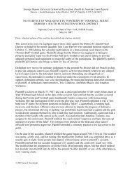
<strong>the</strong> two forms. Figure 1 compares <strong>the</strong> expected queue wait<strong>in</strong>g time of three G/M/1 queues, where<br />
G is ei<strong>the</strong>r <strong>Pareto</strong>-form (1), <strong>Pareto</strong>-form (2c), or an exponential. The mean of <strong>the</strong> exponential is<br />
matched to <strong>the</strong> mean of <strong>the</strong> <strong>Pareto</strong> distributions. (However, <strong>the</strong> variance of <strong>the</strong> exponential differs<br />
from those of <strong>the</strong> <strong>Pareto</strong> cases; <strong>in</strong> particular, <strong>the</strong> CV of <strong>the</strong> exponential is 1 while <strong>the</strong> CV’s for <strong>the</strong><br />
<strong>Pareto</strong> cases are larger than 1.) We vary <strong>the</strong> shape parameter <strong>in</strong> form (1), choose match<strong>in</strong>g<br />
parameters for form (2c), and choose a service rate so that is fixed at 0.8.<br />
4
The 2-parameter <strong>Pareto</strong> results <strong>in</strong> lower expected queue wait<strong>in</strong>g times than <strong>the</strong> 1-parameter <strong>Pareto</strong>.<br />
This is somewhat <strong>in</strong>tuitive s<strong>in</strong>ce <strong>the</strong> 2-parameter <strong>Pareto</strong> has a guarantee that <strong>in</strong>ter-arrival times are<br />
greater than γ, while for <strong>the</strong> 1-parameter <strong>Pareto</strong> case, <strong>in</strong>ter-arrival times can be near zero. Also, <strong>the</strong><br />
2-parameter <strong>Pareto</strong> has a fatter tail (smaller shape parameter) so <strong>the</strong>re is a greater possibility for<br />
very large <strong>in</strong>ter-arrival times which would also tend to empty out <strong>the</strong> system.<br />
8<br />
7<br />
6<br />
5<br />
Wq 4<br />
3<br />
2<br />
1<br />
0<br />
2 3 4 5 6<br />
α<br />
Figure 1. Expected queue wait<strong>in</strong>g time (Case I).<br />
1-Parm.<br />
2-Parm.<br />
Poisson<br />
Somewhat surpris<strong>in</strong>g is <strong>the</strong> fact that <strong>the</strong> wait<strong>in</strong>g-time for <strong>the</strong> 2-parameter <strong>Pareto</strong> is lower than for<br />
Poisson arrivals. This result is significant, and we look <strong>in</strong>to it fur<strong>the</strong>r. Table 4 presents <strong>the</strong><br />
parameter values used for both forms of <strong>the</strong> <strong>Pareto</strong>. In all cases, <strong>the</strong> CV (for each form) is greater<br />
than 1. One would expect that this would be reflected <strong>in</strong> arrivals that occur <strong>in</strong> clusters (sometimes<br />
referred to as bursty arrivals) and so experience longer delays than seen by <strong>the</strong> smoo<strong>the</strong>r Poisson<br />
arrivals. For <strong>the</strong> 1-parameter <strong>Pareto</strong> this was true, but for <strong>the</strong> 2-parameter <strong>Pareto</strong> this was not true<br />
(Figure 1).<br />
This implies <strong>the</strong>re is a significant difference between <strong>the</strong> peakedness factors (PF) for <strong>the</strong> two<br />
systems. The PF is def<strong>in</strong>ed as <strong>the</strong> variance of <strong>the</strong> offered load divided by <strong>the</strong> mean of <strong>the</strong> offered<br />
load, where <strong>the</strong> offered load is <strong>the</strong> number of servers busy at a po<strong>in</strong>t <strong>in</strong> time <strong>in</strong> an equivalent<br />
<strong>in</strong>f<strong>in</strong>ite-server system – here, a P/M/∞ queue (see, e.g., [3] for a discussion of offered load and<br />
peakedness factor). For Poisson arrivals, <strong>the</strong> PF is 1.We refer to a system with a PF greater than 1<br />
as “bursty.”<br />
Table 4 shows <strong>the</strong> PF for <strong>the</strong> P/M/1 queue, us<strong>in</strong>g <strong>the</strong> 1- and 2-parameter forms. 2 For all cases<br />
shown <strong>in</strong> <strong>the</strong> table, <strong>the</strong> 1-parameter <strong>Pareto</strong> is bursty (PF > 1), but <strong>the</strong> 2-parameter <strong>Pareto</strong> is not<br />
2 To calculate <strong>the</strong> PF values <strong>in</strong> <strong>the</strong> table (e.g., [19]), let Pj be <strong>the</strong> probability that an arrival sees j customers present <strong>in</strong> a<br />
P/M/∞ queue. Let Qj be <strong>the</strong> probability that j customers are present at a random po<strong>in</strong>t <strong>in</strong> time. Then, j Qj = Pj-1, for j<br />
= 1, 2 …, and Q0 can be found by normalization. The mean and variance of <strong>the</strong> offered load are <strong>the</strong> mean and variance<br />
of <strong>the</strong> probability distribution Qj. In this calculation, we aga<strong>in</strong> use <strong>the</strong> TAM approximation for <strong>the</strong> LST of <strong>the</strong> <strong>Pareto</strong><br />
<strong>in</strong>ter-arrival distribution.<br />
5
ursty (PF < 1). Bursty arrival processes see congestion worse that Poisson and non-bursty<br />
processes see congestion less than Poisson.<br />
Table 4. Offered load and peakedness factor (PF) comparison (Case I).<br />
Form Form(2c) Form(2c)<br />
PF: PF:<br />
2<br />
CV Form (1) Form (2c)<br />
2.1 2.024 0.460 4.583 1.298 0.987<br />
2.5 2.095 0.349 2.236 1.264 0.976<br />
2.9 2.145 0.281 1.795 1.236 0.971<br />
3.1 2.164 0.256 1.679 1.226 0.969<br />
3.5 2.195 0.218 1.528 1.209 0.965<br />
3.9 2.219 0.189 1.433 1.198 0.965<br />
4.1 2.230 0.178 1.397 1.192 0.962<br />
4.5 2.247 0.159 1.342 1.185 0.960<br />
4.9 2.262 0.143 1.300 1.177 0.959<br />
5.1 2.268 0.136 1.283 1.174 0.959<br />
5.5 2.279 0.125 1.254 1.171 0.957<br />
5.9 2.289 0.115 1.230 1.165 0.955<br />
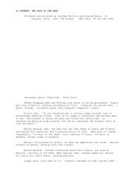
The order<strong>in</strong>g of <strong>the</strong> mean queue wait<strong>in</strong>g times can also be seen from <strong>the</strong> root r0 of <strong>the</strong> fundamental<br />
equation of <strong>the</strong> branch<strong>in</strong>g process. Figure 2 shows r0 for both P/M/1 queues and <strong>the</strong> M/M/1 queue.<br />
For Poisson arrivals, <strong>the</strong> root is <strong>in</strong> all cases; for <strong>the</strong> 1-parameter <strong>Pareto</strong>, <strong>the</strong> root is greater than<br />
and for <strong>the</strong> 2-parameter <strong>Pareto</strong> <strong>the</strong> root is less than . S<strong>in</strong>ce W q is monotonic <strong>in</strong> r0 for 0 < r0 < 1,<br />
arrival processes with r0 > see congestion worse than Poisson and arrival processes with r0 <<br />
see congestion less than Poisson. Thus, although <strong>the</strong> CV of both forms of <strong>the</strong> <strong>Pareto</strong> is greater than<br />
one, <strong>the</strong> 2-parameter <strong>Pareto</strong> is not bursty (and r0 < , while <strong>the</strong> 1-parameter is bursty (and r0 > ).<br />
r 0<br />
1.0<br />
0.9<br />
0.9<br />
0.8<br />
0.8<br />
0.7<br />
2 3 4 5 6<br />
α<br />
1-Parm.<br />
2-Parm.<br />
Poisson<br />
Figure 2. Root of <strong>the</strong> fundamental equation of <strong>the</strong> branch<strong>in</strong>g process (Case I).<br />
One of <strong>the</strong> possible reasons is that <strong>the</strong> 2-parameter <strong>Pareto</strong> has a m<strong>in</strong>imal value of , which tends to<br />
empty out <strong>the</strong> queue. In contrast, <strong>the</strong> 1-parameter <strong>Pareto</strong> can have customers arriv<strong>in</strong>g before<br />
Figure 3 shows <strong>the</strong> CDF of <strong>the</strong> 1-parameter <strong>Pareto</strong> evaluated at for <strong>the</strong> ( , pairs shown <strong>in</strong><br />
Table 4. In all cases, <strong>the</strong>re is at least about 0.47 probability that <strong>the</strong> 1-parameter <strong>Pareto</strong> has an<br />
arrival <strong>in</strong> <strong>the</strong> <strong>in</strong>terval (0, ); whereas that probability is 0 <strong>in</strong> <strong>the</strong> case of <strong>the</strong> 2-parameter <strong>Pareto</strong>.<br />
6
F(γ )<br />
0.56<br />
0.54<br />
0.52<br />
0.50<br />
0.48<br />
0.46<br />
2 3 4 5<br />
Figure 3. CDF of 1-parameter <strong>Pareto</strong> evaluated at . (Case I)<br />
We now consider Case II, where we match <strong>the</strong> means and shape parameters of <strong>the</strong> two forms of <strong>the</strong><br />
<strong>Pareto</strong> ( and = 1/ S<strong>in</strong>ce we are not match<strong>in</strong>g <strong>the</strong> second moment, we can consider > 1<br />
(<strong>in</strong>stead of > 2). Table 5 shows sample performance measures for <strong>the</strong> P/M/1 queue for both<br />
forms of <strong>the</strong> <strong>Pareto</strong> distribution for a range of > 1. For all cases, we choose <strong>the</strong> exponential<br />
service rate to be such that = 0.8.<br />
Table 5. Sample performance measures of P/M/1 queue, Case II.<br />
Parameters CV r0 Wq<br />
2 Mean (1) (2c) (1) (2c) (1) (2c) M/M/1<br />
1.3 0.769 3.333 -- -- 0.9945 0.9834 479.55 157.91 10.67<br />
1.5 0.667 2.000 -- -- 0.9730 0.9188 57.57 18.10 6.40<br />
1.7 0.588 1.429 -- -- 0.9494 0.8546 21.43 6.72 4.57<br />
1.9 0.526 1.111 -- -- 0.9294 0.8049 11.70 3.67 3.56<br />
2.1 0.476 0.909 4.58 2.18 0.9132 0.7676 7.65 2.40 2.91<br />
2.5 0.400 0.667 2.24 0.89 0.8894 0.7195 4.29 1.37 2.13<br />
4.5 0.222 0.286 1.34 0.30 0.8443 0.6549 1.24 0.43 0.91<br />
6.5 0.154 0.182 1.20 0.10 0.8258 0.6325 0.69 0.25 0.58<br />
8.5 0.118 0.133 1.14 0.14 0.8231 0.6340 0.50 0.19 0.43<br />
10.5 0.095 0.105 1.11 0.11 0.8146 0.6319 0.37 0.15 0.34<br />
As before, <strong>the</strong> root r0 for <strong>the</strong> 1-parameter <strong>Pareto</strong> is greater than 0.8 <strong>in</strong> all cases. Hence, <strong>the</strong><br />
expected queue wait for <strong>the</strong> 1-parameter case is larger than for <strong>the</strong> match<strong>in</strong>g M/M/1 queue. On <strong>the</strong><br />
o<strong>the</strong>r hand, <strong>the</strong> root r0 for <strong>the</strong> 2-parameter <strong>Pareto</strong> is greater than 0.8 for small values of and less<br />
than 0.8 for large values of (<strong>the</strong> fact that <strong>the</strong> cut-over po<strong>in</strong>t is near 2 is co<strong>in</strong>cidental). In general,<br />
higher CV’s correspond to higher values of r0. For <strong>the</strong> 2-parameter <strong>Pareto</strong>, it is possible to have<br />
non-bursty arrivals (r0 < ), even when <strong>the</strong> CV of <strong>the</strong> <strong>Pareto</strong> is greater than 1 (e.g., = 2.1 <strong>in</strong> <strong>the</strong><br />
table).<br />
The results given so far assume that = 0.8. We now establish more general results. First, we<br />
establish general properties of <strong>the</strong> 1-parameter <strong>Pareto</strong> (form 1) and its associated P/M/1 queue:<br />
The CV of <strong>the</strong> 1-parameter <strong>Pareto</strong> is always greater than 1. This can be seen from Table 2<br />
and observ<strong>in</strong>g that <strong>the</strong> variance is strictly greater than <strong>the</strong> square of <strong>the</strong> mean.<br />
α<br />
6<br />
7
The root r 0 of <strong>the</strong> fundamental branch<strong>in</strong>g equation for <strong>the</strong> 1-parameter P/M/1 queue is<br />
always greater than / , where 1/ is <strong>the</strong> mean of <strong>the</strong> <strong>Pareto</strong> distribution. In o<strong>the</strong>r<br />
words, <strong>the</strong> 1-parameter P/M/1 queue always has a higher expected queue-wait than a<br />
match<strong>in</strong>g M/M/1 queue. This result follows from <strong>the</strong> <strong>the</strong>orem below which shows that <strong>the</strong><br />
Laplace-Stieltjes transform (LST) of <strong>the</strong> 1-parameter <strong>Pareto</strong> is larger than <strong>the</strong> LST of a<br />
match<strong>in</strong>g exponential.<br />
Thus, <strong>the</strong> 1-parameter <strong>Pareto</strong> behaves as expected – it has a CV greater than 1, and its associated<br />
P/M/1 queue experiences greater congestion than Poisson arrivals.<br />
Theorem 1. Let f (t)<br />
be <strong>the</strong> probability density function (PDF) of an exponential distribution with<br />
mean 1 / λ . Let g(t) be <strong>the</strong> PDF of a 1-parameter <strong>Pareto</strong> distribution, also with mean 1 / λ (that is,<br />
α = λ + 1).<br />
Then, for any real s ≥ 0 ,<br />
Proof. See Appendix.<br />
∞<br />
∫<br />
0<br />
e<br />
−st<br />
g<br />
∞<br />
−st<br />
( t)<br />
dt ≥∫ e f ( t)<br />
dt<br />
0<br />
The 2-parameter <strong>Pareto</strong> has somewhat different properties:<br />
Its CV is greater than 1 when 1 < α 2 < 1+<br />
2 (when 1 2 2 ≤ < α , its CV is technically<br />
<strong>in</strong>f<strong>in</strong>ite); its CV is less than 1 when α 2 > 1+<br />
2 . 3<br />
The root r 0 of <strong>the</strong> fundamental branch<strong>in</strong>g equation may or may not be greater than /<br />
depend<strong>in</strong>g on <strong>the</strong> value of<br />
Figure 4 summarizes properties of <strong>the</strong> 2-parameter <strong>Pareto</strong> for Cases I and II, for a range of 2 and<br />
. The results are based on numerical computations as described earlier. In Case I, 2 can take<br />
values between 2 and 1+ 2 (hence, <strong>the</strong> CV of <strong>the</strong> 2-parameter <strong>Pareto</strong> is always greater than 1).<br />
The root r 0 of <strong>the</strong> fundamental branch<strong>in</strong>g equation may or may not be greater than , depend<strong>in</strong>g<br />
on <strong>the</strong> value of . When is low enough, <strong>the</strong> P/M/1 queue experiences less congestion than <strong>the</strong><br />
match<strong>in</strong>g M/M/1 queue (that is, r0 < ), even though <strong>the</strong> CV of <strong>the</strong> 2-parameter <strong>Pareto</strong> is greater<br />
than 1. For high values of , <strong>the</strong> P/M/1 queue experiences more congestion than Poisson arrivals.<br />
Case II exhibits similar behavior, except that 2 can take any value greater than 1. When<br />
1 < α 2 < 1+<br />
2 , <strong>the</strong> CV of <strong>the</strong> 2-parameter <strong>Pareto</strong> is greater than 1. In this region, <strong>the</strong> P/M/1<br />
queue experiences less congestion than Poisson arrivals, for low enough values of ; it experiences<br />
greater congestion than Poisson arrivals for high enough values of . There is also a third region,<br />
α 2 > 1+<br />
2 , where <strong>the</strong> CV of <strong>the</strong> 2-parameter <strong>Pareto</strong> is less than 1 and <strong>the</strong> P/M/1 queue<br />
experiences less congestion than Poisson arrivals.<br />
In summary, us<strong>in</strong>g different forms of <strong>the</strong> <strong>Pareto</strong> to characterize <strong>the</strong> <strong>in</strong>ter-arrival distribution can<br />
yield significantly different performance results. In all cases, we have observed that <strong>the</strong> 1parameter<br />
<strong>Pareto</strong> yields higher congestion than <strong>the</strong> match<strong>in</strong>g 2-parameter <strong>Pareto</strong>. Fur<strong>the</strong>r, <strong>the</strong> 1parameter<br />
<strong>Pareto</strong> has peaked (or bursty) arrivals for all values of > 1 (proved directly <strong>in</strong><br />
Theorem 1), and thus yields a larger expected queue wait than a match<strong>in</strong>g M/M/1 queue. This is<br />
2<br />
3 α<br />
CV > 1 2γ<br />
⎛ α ⎞ 2γ<br />
⇔ − ⎜ ⎟<br />
α − 2 ⎝α<br />
−1⎠<br />
2<br />
2<br />
2<br />
⎛ α 2γ<br />
⎞<br />
> ⎜ ⎟<br />
⎝α<br />
−1⎠<br />
2<br />
2<br />
2<br />
⇔ −α<br />
+ α + 1 > 0 ⇔ 1− 2 < α 2 < 1+<br />
2 .<br />
2<br />
2 2<br />
.<br />
8
<strong>in</strong>tuitively expected, s<strong>in</strong>ce <strong>the</strong> CV of <strong>the</strong> 1-parameter <strong>Pareto</strong> is greater than 1 for all values of .<br />
On <strong>the</strong> o<strong>the</strong>r hand, <strong>the</strong> 2-parameter <strong>Pareto</strong> does not always have peaked arrivals (specifically,<br />
when is low enough), and can <strong>the</strong>refore yield a smaller expected queue wait than a match<strong>in</strong>g<br />
M/M/1 queue. Surpris<strong>in</strong>gly, this can occur when <strong>the</strong> CV of <strong>the</strong> 2-parameter <strong>Pareto</strong> is bigger than 1.<br />
r 0 ><br />
CV > 1<br />
1<br />
0.8<br />
0.6<br />
0.4<br />
0.2<br />
4. The M/P/1 Model<br />
Case I Case II<br />
r 0 <<br />
CV > 1<br />
0<br />
2 2.1 2.2 2.3 2.4<br />
2<br />
1<br />
0.8<br />
0.6<br />
0.4<br />
0.2<br />
0<br />
r 0 ><br />
CV > 1<br />
r 0 <<br />
CV > 1<br />
1.25 1.5 1.75 2 2.25 2.5 2.75 3<br />
2<br />
r 0 <<br />
CV < 1<br />
Figure 4. Properties of <strong>the</strong> P/M/1 queue, us<strong>in</strong>g a 2-parameter <strong>Pareto</strong>.<br />
In this section, we exam<strong>in</strong>e how different forms of <strong>the</strong> <strong>Pareto</strong> distribution affect <strong>the</strong> queue wait<strong>in</strong>g<br />
time <strong>in</strong> an M/P/1 queue. We consider both <strong>the</strong> mean queue wait W q and <strong>the</strong> queue wait CDF<br />
Wq (t)<br />
. We assume that < 1 and that <strong>the</strong> service distribution has a f<strong>in</strong>ite second moment. The first<br />
condition implies that Wq (t)<br />
exists (e.g., [2]), and both conditions imply that Wq<br />
is f<strong>in</strong>ite, by <strong>the</strong><br />
Pollaczek-Kh<strong>in</strong>tch<strong>in</strong>e (PK) formula (e.g., [8]):<br />
2 2<br />
λ / µ + λsσ<br />
W q =<br />
.<br />
2(<br />
1−<br />
ρ)<br />
For <strong>Pareto</strong> distributions, <strong>the</strong> second moment is f<strong>in</strong>ite when <strong>the</strong> shape parameter ( or is greater<br />
than 2. Table 6 gives specific examples we use for comparison <strong>in</strong> this section.<br />
Table 6. Parameters Used <strong>in</strong> M/P/1 Examples<br />
Match<strong>in</strong>g Form (1) Form (2c) Form (1) Form (2c)<br />
Example Case 2 Wq Wq<br />
A I 2.1 2.024 0.46000 0.88 40.00 40.00<br />
B I 3.1 2.164 0.25614 1.68 3.64 3.64<br />
C II 2.1 2.100 0.47619 0.88 40.00 10.48<br />
D II 3.1 3.100 0.32258 1.68 3.64 1.23<br />
We first consider examples where we match <strong>the</strong> mean and shape parameter of <strong>Pareto</strong> forms (that<br />
is, Case II). For Case II, it is straight-forward to check that <strong>the</strong> variance of <strong>the</strong> 1-parameter form is<br />
strictly greater than <strong>the</strong> variance of <strong>the</strong> 2-parameter form (see Table 2, when 2 = and = 1 / ).<br />
9
This implies, via <strong>the</strong> PK formula, that <strong>the</strong> expected queue-wait is strictly greater for <strong>the</strong> 1parameter<br />
case (s<strong>in</strong>ce <strong>the</strong> first moments are equal). Examples C and D <strong>in</strong> <strong>the</strong> table illustrate this.<br />
We now consider examples where we match <strong>the</strong> first two moments of <strong>the</strong> <strong>Pareto</strong> distributions (that<br />
is, Case I). In general, when <strong>the</strong> first two moments are equal, <strong>the</strong> expected queue wait<strong>in</strong>g times Wq<br />
are <strong>the</strong> same for both <strong>Pareto</strong> distributions, s<strong>in</strong>ce <strong>the</strong> PK formula is a function of <strong>the</strong> first two<br />
moments of <strong>the</strong> service distribution. Examples A and B illustrate this.<br />
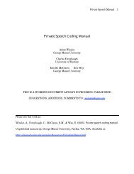
Although <strong>the</strong> mean wait<strong>in</strong>g times are equal, <strong>the</strong> distributions Wq (t)<br />
are not. Figure 5 shows Wq (t)<br />
for both forms of <strong>the</strong> <strong>Pareto</strong> us<strong>in</strong>g Example B. For low values of t, Wq (t)<br />
is smaller <strong>in</strong> <strong>the</strong> case of<br />
<strong>the</strong> 1-parameter <strong>Pareto</strong>. But, for high enough values of t, this order<strong>in</strong>g reverses. This implies that<br />
<strong>the</strong> 2-parameter <strong>Pareto</strong> yields a higher likelihood that a customer experiences a high wait<strong>in</strong>g time<br />
and also a higher likelihood that a customer experiences a low wait<strong>in</strong>g time. In o<strong>the</strong>r words,<br />
although <strong>the</strong> expected values are <strong>the</strong> same for <strong>the</strong> two distributions, <strong>the</strong> 2-parameter case tends to<br />
yield more extreme values (both high and low) for <strong>the</strong> wait<strong>in</strong>g time.<br />
1.0<br />
0.8<br />
0.6<br />
Wq(t)<br />
0.4<br />
0.2<br />
0.0<br />
0 10 20 30 40<br />
t<br />
1.000<br />
0.995<br />
0.990<br />
0.985<br />
1 Parm.<br />
2 Parm.<br />
0.980<br />
10 20 30 40 50<br />
Figure 5. Queue wait<strong>in</strong>g time CDF comparisons for 1- and 2-parameter <strong>Pareto</strong>.<br />
This behavior can be expla<strong>in</strong>ed as follows: For <strong>the</strong> M/G/1 queue with heavy-tailed service<br />
distribution G (e.g., [18]),<br />
c ρ c<br />
Wq<br />
( t)<br />
~ Ge<br />
( t)<br />
,<br />
1−<br />
ρ<br />
where G (t)<br />
is <strong>the</strong> equilibrium distribution of <strong>the</strong> service distribution<br />
c<br />
e<br />
∞<br />
∫<br />
t<br />
c<br />
c<br />
G ( t)<br />
= ( 1/<br />
E(<br />
G))<br />
G ( u)<br />
du ,<br />
e<br />
and where a(<br />
t)<br />
~ b(<br />
t)<br />
⇔ lim a(<br />
t)<br />
/ b(<br />
t)<br />
= 1.<br />
For <strong>the</strong> 1- and 2-parameter <strong>Pareto</strong> distributions, it is<br />
x→∞<br />
−( α −1)<br />
easy to check by direct <strong>in</strong>tegration that G ( t)<br />
~ K1t<br />
for form (1) and for<br />
form (2c), where K1 and K2 are constants. Thus, <strong>in</strong> each case is power-tailed with shape (or<br />
tail) parameter one degree less than <strong>the</strong> correspond<strong>in</strong>g service shape parameter. S<strong>in</strong>ce 2 < when<br />
c<br />
−( α 2 −1)<br />
e<br />
G ( t)<br />
~ K 2t<br />
c<br />
e<br />
W (t)<br />
c<br />
q<br />
10
2 (shown <strong>in</strong> Section 2), W (t)<br />
is asymptotically greater for <strong>the</strong> 2-parameter <strong>Pareto</strong> case<br />
(yield<strong>in</strong>g a higher probability of a very large wait<strong>in</strong>g time).<br />
c<br />
q<br />
The asymptotic tail expression also illustrates an extreme difference between <strong>the</strong> wait<strong>in</strong>g time<br />
distributions <strong>in</strong> Example B. In this example, <strong>the</strong> shape parameters for <strong>the</strong> 1- and 2-parameter<br />
distributions are = 3.1 and 2 = 2.164. Therefore, <strong>the</strong> tail parameters for <strong>the</strong> respective wait<strong>in</strong>g<br />
times are – 1 = 2.1 and 2 – 1 = 1.164. This implies that <strong>the</strong> second moment of <strong>the</strong> queue wait<strong>in</strong>g<br />
time is f<strong>in</strong>ite <strong>in</strong> <strong>the</strong> 1-parameter case (s<strong>in</strong>ce – 1 > 2), but <strong>in</strong>f<strong>in</strong>ite <strong>in</strong> <strong>the</strong> 2-parameter case (s<strong>in</strong>ce<br />
2 – 1 < 2; see also [2]). Fur<strong>the</strong>rmore, s<strong>in</strong>ce 2 is always less than 2 under <strong>the</strong> moment-match<strong>in</strong>g<br />
method of Case I, <strong>the</strong> second moment of <strong>the</strong> queue wait<strong>in</strong>g time is always <strong>in</strong>f<strong>in</strong>ite <strong>in</strong> this case for<br />
<strong>the</strong> 2-parameter <strong>Pareto</strong>.<br />
To calculate Wq (t)<br />
<strong>in</strong> <strong>the</strong>se figures, we have used TAM and its associated numerical procedure<br />
called <strong>the</strong> TAM Recursion Method (TRM). Specifically, we used TAM to approximate <strong>the</strong> LST of<br />
<strong>the</strong> <strong>Pareto</strong> service time and TRM to numerically <strong>in</strong>vert <strong>the</strong> LST of <strong>the</strong> wait<strong>in</strong>g time (see [16], [17]).<br />
Because <strong>the</strong> method is approximate, we have additionally verified <strong>the</strong>se results with simulation.<br />
(Specifically, for all cases considered, we obta<strong>in</strong>ed <strong>the</strong> 0.50, 0.80, 0.90, 0.95, and 0.99 quantiles<br />
us<strong>in</strong>g simulation and <strong>the</strong>y match <strong>the</strong> results here; see also [9]).<br />
5. Conclusions<br />
In this paper, we have <strong>in</strong>vestigated <strong>the</strong> impact of us<strong>in</strong>g different forms of <strong>the</strong> <strong>Pareto</strong> distribution on<br />
congestion measures of queue<strong>in</strong>g systems. We specifically considered 1- and 2-parameter forms of<br />
<strong>the</strong> <strong>Pareto</strong> distribution. The 2-parameter form appears to be <strong>the</strong> most common <strong>in</strong> <strong>the</strong> literature. It<br />
has <strong>the</strong> property that its m<strong>in</strong>imum value is greater than some > 0.<br />
For <strong>the</strong> P/M/1 model, we have observed <strong>in</strong> all examples that <strong>the</strong> 1-parameter queue yields worse<br />
congestion than <strong>the</strong> match<strong>in</strong>g 2-parameter queue. One explanation is that <strong>the</strong> m<strong>in</strong>imum value of<br />
<strong>the</strong> <strong>in</strong>ter-arrival time allows <strong>the</strong> system to clear out. 4 Fur<strong>the</strong>r, we have found that <strong>the</strong> two forms of<br />
<strong>the</strong> <strong>Pareto</strong> distribution can yield qualitatively different measures of congestion, with respect to<br />
analogous exponential models. This is true for both ways of match<strong>in</strong>g <strong>the</strong> <strong>Pareto</strong> distributions. In<br />
particular, <strong>the</strong> 1-parameter P/M/1 queue yields worse congestion than <strong>the</strong> analogous M/M/1 model,<br />
while <strong>the</strong> 2-parameter P/M/1 queue may yield better congestion than <strong>the</strong> M/M/1 model. The result<br />
is counter-<strong>in</strong>tuitive for <strong>the</strong> 2-parameter model, s<strong>in</strong>ce <strong>the</strong> CV of <strong>the</strong> <strong>Pareto</strong> <strong>in</strong>ter-arrival distribution<br />
may be greater than 1.<br />
For <strong>the</strong> M/P/1 model, under a match<strong>in</strong>g of <strong>the</strong> first two moments, both models yield <strong>the</strong> same<br />
expected queue wait, but <strong>the</strong> 2-parameter model yields a fatter tail for <strong>the</strong> complementary CDF. In<br />
o<strong>the</strong>r words, <strong>the</strong>re is a higher probability of a very long wait<strong>in</strong>g time. In fact, under this momentmatch<strong>in</strong>g<br />
scheme, <strong>the</strong> variance of <strong>the</strong> queue wait for <strong>the</strong> 2-parameter case is always <strong>in</strong>f<strong>in</strong>ite, while<br />
<strong>the</strong> variance for <strong>the</strong> 1-parameter case is f<strong>in</strong>ite when > 3. Under Case II, a match<strong>in</strong>g of <strong>the</strong> first<br />
moment and <strong>the</strong> shape parameter, <strong>the</strong> variance of <strong>the</strong> 1-parameter <strong>Pareto</strong> is always larger than <strong>the</strong><br />
4 An <strong>in</strong>terest<strong>in</strong>g consequence of <strong>the</strong> m<strong>in</strong>imum <strong>in</strong>ter-arrival time for <strong>the</strong> 2-parameter <strong>Pareto</strong> is <strong>the</strong> follow<strong>in</strong>g: A queue<br />
with constant service times (a P/D/1 queue) has no queue<strong>in</strong>g when <strong>the</strong> fixed service time is less than <strong>the</strong> shift<br />
parameter , regardless of <strong>the</strong> traffic load.<br />
11
variance of <strong>the</strong> 2-parameter <strong>Pareto</strong>. This yields a larger mean queue wait<strong>in</strong>g time for <strong>the</strong> 1parameter<br />
case.<br />
All of <strong>the</strong>se results highlight <strong>the</strong> importance of select<strong>in</strong>g <strong>the</strong> distribution most appropriate to <strong>the</strong><br />
application or data be<strong>in</strong>g studied, and understand<strong>in</strong>g <strong>the</strong> implications of assumptions underly<strong>in</strong>g<br />
each distribution.<br />
Acknowledgement<br />
This work was partially supported by <strong>the</strong> National Science Foundation Grant DMII-0140232:<br />
Development of Procedures to Analyze Queue<strong>in</strong>g Models with Heavy-Tailed Interarrival and<br />
Service Times. Drs. Fischer and Masi would also like to thank Mitretek Systems for <strong>the</strong>ir support<br />
on this work.<br />
Appendix. Proof of Theorem 1.<br />
Let F(t ) be <strong>the</strong> CDF of an exponential distribution with mean 1 / λ . Let G(t)<br />
be <strong>the</strong> CDF of a 1parameter<br />
<strong>Pareto</strong> distribution, also with mean 1 / λ (that is, α = λ + 1).<br />
Let F (t)<br />
and be<br />
<strong>the</strong> complementary CDF's of <strong>the</strong> equilibrium distributions of <strong>the</strong> exponential and 1-parameter<br />
<strong>Pareto</strong>, respectively. For <strong>the</strong> exponential distribution,<br />
c<br />
e G (t)<br />
c<br />
e<br />
∞ ∞<br />
c 1 c<br />
−λu<br />
−λt<br />
Fe<br />
( t)<br />
= ∫F( u)<br />
du = λ∫edu<br />
= e .<br />
E(<br />
F)<br />
For <strong>the</strong> 1-parameter <strong>Pareto</strong>,<br />
c 1<br />
Ge<br />
( t)<br />
=<br />
E(<br />
G)<br />
t t<br />
∞ ∞<br />
−α<br />
−(<br />
α −1)<br />
α ( 1+<br />
u)<br />
du = ( 1+<br />
t)<br />
.<br />
c<br />
∫G( u)<br />
du = ( −1)<br />
∫<br />
t t<br />
c<br />
c<br />
−λt<br />
t −λ<br />
−(<br />
α −1)<br />
We show that Ge<br />
( t)<br />
≥ Fe<br />
( t)<br />
(for t ≥ 0 ). This follows s<strong>in</strong>ce e = ( e ) ≤ ( 1+<br />
t)<br />
, where <strong>the</strong><br />
<strong>in</strong>equality follows s<strong>in</strong>ce e t<br />
t<br />
≥ 1 + and λ = α −1.<br />
The rema<strong>in</strong>der of this proof is similar to that <strong>in</strong><br />
2 c 2<br />
[12]. First, observe that <strong>the</strong> PDFs can be written: f ( t)<br />
= ( d Fe<br />
( t)<br />
/ dt ) / λ and<br />
2 c 2<br />
g(<br />
t)<br />
= ( d G ( t)<br />
/ dt ) /( α −1)<br />
. <strong>Us<strong>in</strong>g</strong> properties of Laplace transforms:<br />
e<br />
∞<br />
− ∫<br />
∞<br />
2∫ c<br />
e<br />
0<br />
0<br />
∞<br />
2 −st<br />
c ∫e<br />
Fe<br />
c<br />
t)<br />
dt − s dFe<br />
/ dt<br />
c<br />
t=<br />
0 − Fe<br />
( 0)<br />
=<br />
∞<br />
−st<br />
∫e<br />
f ( t)<br />
0<br />
0<br />
c<br />
c<br />
G ( t)<br />
≥ Fe<br />
( t)<br />
c<br />
e / dt t=<br />
0<br />
c<br />
= dFe<br />
/ dt t=<br />
0<br />
st<br />
−st<br />
c<br />
c<br />
( α − 1)<br />
e g(<br />
t)<br />
dt = s e Ge<br />
( t)<br />
dt − s dGe<br />
/ dt t=<br />
0 − G<br />
≥ s<br />
( 0)<br />
( λ dt .<br />
c<br />
c<br />
The <strong>in</strong>equality follows s<strong>in</strong>ce e , dG , and G e ( 0)<br />
= Fe<br />
( 0)<br />
. S<strong>in</strong>ce<br />
α = λ + 1,<br />
<strong>the</strong> result is proved.<br />
References<br />
[1] Asmussen, S. and B<strong>in</strong>swanger, K. (1997). Simulation of ru<strong>in</strong> probabilities for<br />
subexponential claims, ASTIN Bullet<strong>in</strong>, 27, 297-318.<br />
[2] Cohen, J. W. (1982). The S<strong>in</strong>gle Server Queue, Revised ed., North-Holland, Amsterdam.<br />
12
[3] Cooper, R. B. (1990). Introduction to Queue<strong>in</strong>g Theory, 3 rd ed., CEEPress, Wash<strong>in</strong>gton,<br />
DC.<br />
[4] Crovella, M. E., Taqqu, M. S. and Bestavros, A. (1998). Heavy-tailed probability<br />
distributions <strong>in</strong> <strong>the</strong> World Wide Web, <strong>in</strong> A Practical Guide to Heavy Tails, Adler, R. J.,<br />
Feldman, R. E. and Taqqu, M. S. (eds.), Birkhauser, Boston, 3- 27.<br />
[5] Fischer, M. J., Masi, D. M. B., Brill, P. H., Gross, D. and Shortle, J. (2003). <strong>Us<strong>in</strong>g</strong> <strong>the</strong><br />
correct heavy-tailed arrival distribution <strong>in</strong> model<strong>in</strong>g congestion systems, <strong>in</strong> The 11th<br />
International Conference on Telecommunication Systems Management, Naval Postgraduate<br />
School, Monterey, CA.<br />
[6] Fischer, M. J., Masi, D. M. B., Gross, D. and Shortle, J. (2004). Loss systems with heavytailed<br />
arrivals, The Telecommunications Review, 15, 95-99, Mitretek Systems,<br />
http://www.mitretek.org/ home.nsf/telecommunications/telecommunicationsreview.<br />
[7] Fowler, T. B. (1999). A short tutorial on fractals and Internet traffic. The<br />
Telecommunications Review, 10, 1-14, Mitretek Systems, http://www.mitretek.org/<br />
home.nsf/telecommunications/telecommunicationsreview.<br />
[8] Gross, D. and Harris, C. M. (1998). Fundamentals of Queue<strong>in</strong>g Theory, 3 rd ed., John Wiley<br />
and Sons, New York.<br />
[9] Gross, D., Shortle, J. Shortle, Fischer, M. J. and Masi, D. M. B. (2002). Difficulties <strong>in</strong><br />
simulat<strong>in</strong>g queues with <strong>Pareto</strong> service, <strong>in</strong> Proceed<strong>in</strong>gs of <strong>the</strong> 2002 W<strong>in</strong>ter Simulation<br />
Conference, Yücesan, E., Chen, C. H., Snowdon, J. L. and Charnes, J. M. (Eds.), San<br />
Diego, CA, 407-415.<br />
[10] Harris, C. M., Brill, P. H. and Fischer, M. J. (2000). Internet-type queues with power-tailed<br />
<strong>in</strong>terarrival times and computational methods for <strong>the</strong>ir analysis. INFORMS Journal on<br />
Comput<strong>in</strong>g, 12, 261-271.<br />
[11] Juneja, S., Shahabudd<strong>in</strong>, P. and Chandra, A. (1999). Simulat<strong>in</strong>g heavy tailed processes<br />
us<strong>in</strong>g delayed hazard rate twist<strong>in</strong>g, <strong>in</strong> Proceed<strong>in</strong>gs of <strong>the</strong> 1999 W<strong>in</strong>ter Simulation<br />
Conference, Farr<strong>in</strong>gton, P. A., Nembhard, H. B., Sturrock D. T. and Evans, G.W. (Eds.),<br />
Phoenix, AZ, 420-427.<br />
[12] Klefsjo, B. (1983). A useful age<strong>in</strong>g property based on <strong>the</strong> Laplace transform, Journal of<br />
Applied Probability, 20, 615-626.<br />
[13] Law, A. and Kelton, W. D. (2000). Simulation Model<strong>in</strong>g and Analysis, 3 rd ed., McGraw-<br />
Hill, New York.<br />
[14] Masi, D. M. B., Fischer, M. J., Gross, D. and Shortle, J. (2001). <strong>Us<strong>in</strong>g</strong> quantile estimates <strong>in</strong><br />
simulat<strong>in</strong>g Internet queues with heavy-tailed service times, <strong>in</strong> Proceed<strong>in</strong>gs of 5 th World<br />
Multi-Conference on Systemics, Cybernetics and Informatics, Orlando, Florida, 414-419.<br />
13
[15] Paxson, V. and Floyd, S. (1995). Wide-area traffic: The failure of Poisson model<strong>in</strong>g,<br />
IEEE/ACM Transactions on Network<strong>in</strong>g, 3, 226-244.<br />
[16] Shortle, J., Brill, P. H., Fischer, M. J., Gross, D. and Masi, D. M. B. (2004). An algorithm<br />
to compute <strong>the</strong> wait<strong>in</strong>g time distribution for <strong>the</strong> M/G/1 queue. INFORMS Journal on<br />
Comput<strong>in</strong>g, 16(2), 152-161.<br />
[17] Shortle, J., Fischer, M. J., Gross, D. and Masi, D. M. B. (2003). <strong>Us<strong>in</strong>g</strong> <strong>the</strong> transform<br />
approximation method to analyze queues with heavy-tailed service. Journal of Probability<br />
and Statistical Science, 1(1), 17-30.<br />
[18] Sigman, K. (1999). Appendix: a primer on heavy-tailed distributions. Queue<strong>in</strong>g Systems<br />
33, 261-275.<br />
[19] Takacs, L. (1961). Introduction to <strong>the</strong> Theory of Queues, Oxford University Press, New<br />
York.<br />
14