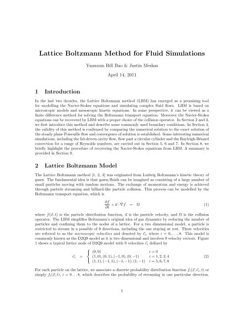
Lattice Boltzmann Method for Fluid Simulations

Lattice Boltzmann Method for Fluid Simulations
1 Introduction
Yuanxun Bill Bao & Justin Meskas
April 14, 2011
In the last two decades, the Lattice Boltzmann method (LBM) has emerged as a promising tool
for modelling the Navier-Stokes equations and simulating complex fluid flows. LBM is based on
microscopic models and mesoscopic kinetic equations. In some perspective, it can be viewed as a
finite difference method for solving the Boltzmann transport equation. Moreover the Navier-Stokes
equations can be recovered by LBM with a proper choice of the collision operator. In Section 2 and 3,
we first introduce this method and describe some commonly used boundary conditions. In Section 4,
the validity of this method is confirmed by comparing the numerical solution to the exact solution of
the steady plane Poiseuille flow and convergence of solution is established. Some interesting numerical
simulations, including the lid-driven cavity flow, flow past a circular cylinder and the Rayleigh-Bénard
convection for a range of Reynolds numbers, are carried out in Section 5, 6 and 7. In Section 8, we
briefly highlight the procedure of recovering the Navier-Stokes equations from LBM. A summary is
provided in Section 9.
2 Lattice Boltzmann Model
The Lattice Boltzmann method [1, 2, 3] was originated from Ludwig Boltzmann’s kinetic theory of
gases. The fundamental idea is that gases/fluids can be imagined as consisting of a large number of
small particles moving with random motions. The exchange of momentum and energy is achieved
through particle streaming and billiard-like particle collision. This process can be modelled by the
Boltzmann transport equation, which is
∂f
∂t
+ u · ∇f = Ω (1)
where f(x, t) is the particle distribution function, u is the particle velocity, and Ω is the collision
operator. The LBM simplifies Boltzmann’s original idea of gas dynamics by reducing the number of
particles and confining them to the nodes of a lattice. For a two dimensional model, a particle is
restricted to stream in a possible of 9 directions, including the one staying at rest. These velocities
are referred to as the microscopic velocities and denoted by ei, where i = 0, . . . , 8. This model is
commonly known as the D2Q9 model as it is two dimensional and involves 9 velocity vectors. Figure
1 shows a typical lattice node of D2Q9 model with 9 velocities ei defined by
ei =
⎧
⎨
⎩
(0, 0) i = 0
(1, 0), (0, 1), (−1, 0), (0, −1) i = 1, 2, 3, 4
(1, 1), (−1, 1), (−1, −1), (1, −1) i = 5, 6, 7, 8
For each particle on the lattice, we associate a discrete probability distribution function fi(x, ei, t) or
simply fi(x, t), i = 0 . . . 8, which describes the probability of streaming in one particular direction.
1
(2)

Figure 1: Illustration of a lattice node of the D2Q9 model
The macroscopic fluid density can be defined as a summation of microscopic particle distribution
function,
ρ(x, t) =
8
fi(x, t) (3)
Accordingly, the macroscopic velocity u(x, t) is an average of microscopic velocities ei weighted by
the distribution functions fi,
i=0
u(x, t) = 1
ρ
8
cfiei
The key steps in LBM are the streaming and collision processes which are given by
fi(x + cei∆t, t + ∆t) − fi(x, t)
Streaming
i=0
= − [fi(x, t) − f eq
i (x, t)]
τ
Collision
In the actual implementation of the model, streaming and collision are computed separately, and special
attention is given to these when dealing with boundary lattice nodes. Figure 2 shows graphically
how the streaming step takes place for the interior nodes.
Figure 2: Illustration of the streaming process of a lattice node
In the collision term of (5), f eq
i (x, t) is the equilibrium distribution, and τ is considered as the relaxation
time towards local equilibrium. For simulating single phase flows, it suffices to use Bhatnagar-
Gross-Krook (BGK) collision, whose equilibrium distribution f eq
i is defined by
f eq
i (x, t) = wiρ + ρsi(u(x, t)) (6)
2
(4)
(5)

where si(u) is defined as
and wi, the weights,
si(u) = wi
wi =
3 ei · u
c
⎧
⎨
⎩
9 (ei · u)
+
2
2
c2 − 3
2
4/9 i = 0
1/9 i = 1, 2, 3, 4
1/36 i = 5, 6, 7, 8
u · u
c2
, (7)
and c = ∆x
is the lattice speed. The fluid kinematic viscosity ν in the D2Q9 model is related to the
∆t
relaxation time τ by
ν =
The algorithm can be summarized as follows:
1. Initialize ρ, u, fi and f eq
i
2τ − 1 (∆x)
6
2
∆t
2. Streaming step: move fi −→ f ∗ i in the direction of ei
3. Compute macroscopic ρ and u from f ∗ i
4. Compute f eq
i
using (6)
using (3) and (4)
5. Collision step: calculate the updated distribution function fi = f ∗ i
6. Repeat step 2 to 5
− 1
τ (f ∗ i − f eq
i
) using (5)
Notice that numerical issues can arise as τ → 1/2. During the streaming and collision step, the
boundary nodes require some special treatments on the distribution functions in order to satisfy the
imposed macroscopic boundary conditions. We discuss these in details in Section 3.
3 Boundary Conditions
Boundary conditions (BCs) are central to the stability and the accuracy of any numerical solution.
For the lattice Boltzmann method, the discrete distribution functions on the boundary have to be
taken care of to reflect the macroscopic BCs of the fluid. In this project, we explore two of the most
widely used BCs: Bounce-back BCs [4] and Zou-He velocity and pressure (density) BCs [5].
3.1 Bounce-back BCs
Bounce-back BCs are typically used to implement no-slip conditions on the boundary. By the so-called
bounce-back we mean that when a fluid particle (discrete distribution function) reaches a boundary
node, the particle will scatter back to the fluid along with its incoming direction. Bounce-back BCs
come in a few variants and we focus on two types of implementations: the on-grid and the mid-grid
bounce-back [4].
The idea of the on-grid bounce-back is particularly simple and preserves a decent numerical accuracy.
In this configuration, the boundary of the fluid domain is aligned with the lattice points (see Figure
3). One can use a boolean mask for the boundary and the interior nodes. The incoming directions
of the distribution functions are reversed when encountering a boundary node. This implementation
3
(8)
(9)

Figure 3: Illustration of on-grid bounce-back
does not distinguish the orientation of the boundaries and is ideal for simulating fluid flows in complex
geometries, such as the porous media flow.
The configuration of the mid-grid bounce-back introduces fictitious nodes and places the boundary
wall centered between fictitious nodes and boundary nodes of the fluid (see Figure 4). At a given
time step t, the distribution functions with directions towards the boundary wall would leave the
domain. Collision process is then applied and directions of these distribution functions are reversed
and they bounce back to the boundary nodes. We point out that the distribution functions at the
end of bounce-back in this configuration is the post-collision distribution functions.
Figure 4: Illustration of mid-grid bounce-back
Although the on-grid bounce-back is easy to implement, it has been verified that it is only first-order
accurate due to its one-sided treatment on streaming at the boundary. However the centered nature
of the mid-grid bounce-back leads to a second order of accuracy at the price of a modest complication.
3.2 Zou-He Velocity and Pressure BCs
In many physical situations, we would like to model flows with prescribed velocity or pressure (density)
at the boundary. This particular velocity/pressure BC we discuss here was originally developed by Zou
and He in [5]. For illustration, we consider that the velocity uL = (u, v) is given on the left boundary.
After streaming, f0, f2, f3, f4, f6 and f7 are known. What’s left undetermined are f1, f5, f8 and ρ (see
Figure 5).
4

Figure 5: Illustration of Zou-He velocity BC
The idea of Zou-He BCs is to formulate a linear system of f1, f5, f8 and ρ using (3) and (4). After
rearranging:
By considering (10) and (11), we can determine
f1 + f5 + f8 = ρ − (f0 + f2 + f4 + f3 + f6 + f7) (10)
f1 + f5 + f8 = ρu + (f3 + f6 + f7) (11)
f5 − f8 = ρv − f2 + f4 − f6 + f7 (12)
ρ =
1
1 − u [(f0 + f2 + f4 + 2(f3 + f6 + f7)] (13)
However, we need a fourth equation to close the system and solve for f1, f5 and f8. The assumption
made by Zou and He is that the bounce-back rule still holds for the non-equilibrium part of the
particle distribution normal to the boundary. In this case, the fourth equation is
f1 − f eq
1 = f3 − f eq
3
With f1 solved by (6) and (14), f5, f8 are subsequently determined:
(14)
f1 = f3 + 2
ρv
3
(15)
f5 = f7 − 1
2 (f2 − f4) + 1 1
ρu + ρv
6 2
(16)
f8 = f6 + 1
2 (f2 − f4) + 1 1
ρu − ρv
6 2
(17)
A similar procedure is taken if a given pressure (density) is imposed on the boundary. Here we notice
that this type of BC depends on the orientation of the boundary and thus is hard to generalize for
complex geometries.
5

4 Steady Plane Poiseuille Flow
In this simulation we apply the lattice BGK model in Section 2 to solve the steady plane Poiseuille
flow. The flow is steady and in driven by a pressure gradient at the inlet and the outlet of the channel
(see Figure 6).
Figure 6: Plane Poiseuille flow
By using symmetry and incompressibility, the velocity components u, v do not have any horizontal
variation and v ≡ 0. The Navier-Stokes equations are further reduced to
where ∂p
∂x = P1 − P0
. The initial and boundary conditions are
L
µ ∂2u ∂p
= , (18)
∂y2 ∂x
u(x, y, 0) = v(x, y, 0) = 0; p(x, y, 0) = Pavg
u(x, 0, t) = v(x, 0, t) = 0; u(x, H, t) = v(x, H, t) = 0
p(0, y, t) = P0; p(L, y, t) = P1
where Pavg = (P0 + P1)/2, and P0 and P1 are the pressure at the inlet and the outlet of the channel.
The steady Poiseuille flow has the exact solution for velocity:
u(x, y, t) = ∆p
y(y − H)
2µL
(19)
v(x, y, t) = 0 (20)
For the simulation, we apply periodic BCs at the inlet and the outlet. Both mid-grid and on-grid
BCs are implemented on the top and bottom plates and compared for convergence. We take L = 40,
H = 32, ∆p = −0.05, τ = 1. The criterion of steady state is
ij
|u n+1
ij
ij
− un ij|
|u n+1
ij |
≤ 5.0 × 10 −9
where u n ij is the horizontal velocity component on (xi, yj) at the n th time step.
The left graph of Figure 7 shows that the computed velocity profile agrees closely with the analytical
solution. The first order convergence of on-grid bounce-back and the second order convergence of midgrid
bounce-back, discussed in Section 3.1, have been validated for this problem in the convergence
plot.
6
(21)

y
35
30
25
20
15
10
5
parabolic velocity profile
LBM
Analytical
0
0 1 2 3 4 5
u(y)
6 7 8 9 10
error
10 1
10 2
10 3
10 4
10 5
10 0
convergence of bounceback boundary conditions
Figure 7: Parabolic velocity profile of plane Poiseuille flow and convergence of solution
5 Lid-Driven Cavity Flow
10 1
N
midgrid
ongrid
2nd order
1st order
In this simulation we have a 2D fluid flow that is driven by a lid at the top which moves at a speed of
u(x, 1, t) = Vd in the right direction. The other three walls have bounce-back BCs for the distribution
function and no-slip BCs for the velocity, u = 0 and v = 0. The moving lid has Zou-He BCs . The
initial conditions state that the velocity field is zero everywhere and the initial distribution function
is set by the weights, fi = wi. This results in an initial condition that ρ = 1 from (3). The only
exception is the velocity of the fluid on the top is set to be Vd.
Figure 8: Color plot of the norm of the velocity: Re = 1000, ν = 1/18, τ = 2/3, 256 × 256 lattice
The two top corner lattice points are singular points and are considered as part of the moving lid.
Simulations were done with a 256 × 256 lattice, ν = 1/18, τ = 2/3 and with Re = 400 and 1000.
Figure 8 shows a color visualization of the simulation for Re = 1000.
7
10 2

y
1
0.9
0.8
0.7
0.6
0.5
0.4
0.3
0.2
0.1
Stream Trace for Re = 400
0
0 0.2 0.4 0.6 0.8 1
x
y
1
0.9
0.8
0.7
0.6
0.5
0.4
0.3
0.2
0.1
Stream Trace for Re = 1000
0
0 0.2 0.4 0.6 0.8 1
x
Figure 9: Stream traces for Re = 400 and 1000, ν = 1/18, τ = 2/3, 256 × 256 lattice
From the stream traces of Figure 9 the simulation produces similar vortex-like behavior as a real
physical flow, with a clockwise center vortex and a counter-clockwise secondary vortex in the right
bottom corner. With higher Re a third counter-clockwise vortex is visible in the left bottom corner.
6 Flow Past A Circular Cylinder
The study of flow past an object dates its history back to aircraft design in the early 20th century.
Researchers were interested in the design of wings of an aircraft and understanding the behavior of
the flow past them. It turns out that the Reynolds number plays an important role in characterizing
the behavior of the flow.
Figure 10: Illustration of flow past a cylinder
In this simulation, we set up a 2D channel with a steady Poiseuille flow. A circular cylinder is then
immersed into the flow at the start of the simulation. On-grid bounce-back BCs are applied on the
cylinder as well as the top and the bottom plates. Zou-He velocity and pressure (density) BCs are
implemented at the inlet and the outlet of the flow (see Figure 10).
8

Simulations with Re = 5, 40, 150 have been carried out and the behavior of the flow is matched with
images from laboratory experiments. The results are summarized in the following figures.
• Re < 5: a smooth laminar flow across the cylinder
Figure 11: Re = 5: Laminar flow past a cylinder: simulation vs experiment
• 5 < Re < 40: a pair of fixed symmetric vortices generated at the back of the cylinder
Figure 12: Re = 40: A fixed pair of vortices: simulation vs experiment
• 40 < Re < 400: Vortex streets
Figure 13: Streamlines of flow at Re = 150
9

Figure 14: Vorticity plot of flow past a cylinder at Re = 150, a Karman vortex street is generated
7 Rayleigh-Bénard convection
Rayleigh-Bénard convection is a type of natural convection, in which the fluid motion is not purely
driven by an external force, but also by density differences in the fluid due to temperature gradients.
A very important implication of convection is the ocean-atmosphere dynamics, where heated air or
water vapor upwell from the ocean into the atmosphere and this is fundamental in understanding
climate patterns such as El Niño and La Niña.
The Boussinesq approximation is often used in the study of natural convection. With this approximation,
density is assumed to be constant except for the buoyancy term in the equations of motion.
The governing equations are
10

∇ · u = 0 (22)
Du
Dt
=
1
− ∇p + ν∇
ρ0
2 u + ρ
g
ρ0
(23)
DT
Dt = κ∇2T (24)
where u is the fluid velocity, ν is the kinematic viscosity, ρ is the density variation, ρ0 is the constant
ambient fluid density, T is the temperature and κ is the thermal diffusivity constant. Furthermore
the density ρ is assumed to be linearly related to the temperature T :
ρ = ρ0(1 − β(T − T0)) (25)
Here T0 is the average fluid temperature and β is the coefficient of thermal expansion.
By putting (25) into (23) and absorbing the first term of ρ into the pressure term, we get the following
coupled equations between velocity and temperature:
∇ · u = 0 (26)
Du
Dt
=
1
− ∇p + ν∇
ρ0
2 u − gβ(T − T0) (27)
DT
Dt = κ∇2T (28)
An important observation is that T appears as a buoyancy force in the momentum equation (27).
Thus the Boussinesq equations (26)-(28) can be simulated by two independent BGK models with a
buoyancy forcing term coupling the two models. For velocity u, a modified BGK model (ID2Q9) with
much less compressible effects is applied in [6]. This model is based on the same D2Q9 lattice but
uses pressure p instead of density ρ as a primitive variable. A new microscopic distribution function
gi(x, t) is introduced along with its equilibrium distribution function geq (x, t) defined by
g eq (x, t) =
where si(u) is defined as before in (7).
⎧
⎪⎨
⎪⎩
−4σ p
c 2 + s1(u) i = 0
λ p
c 2 + si(u) i = 1, 2, 3, 4
γ p
c 2 + si(u) i = 5, 6, 7, 8
The evolution equation of the distribution function gi(x, t) is similar to (5),
(29)
gi(x + cei∆t, t + ∆t) = gi(x, t) − 1
τ (gi − g eq
i ) (30)
The relaxation time τ is related to kinematic viscosity ν through
ν =
2τ − 1 (∆x)
6
2
∆t
The marcoscopic velocity u and pressure p are given by
8
u = ceigi, p = c2
8
gi + s0(u)
4σ
i=0
11
i=1
(31)
(32)

It can be shown rigorously that the incompressible Navier-Stokes equation can be derived from this
discrete model using a multiscaling expansion with an error of O(∆t 2 ) [1].
A simple D2Q4 BGK model is used to simulate the advection-diffusion of temperature. A lattice
with four discrete velocity directions e1, e2, e3 and e4 as defined in (2) is implemented. The evolution
equations of the temperature distribution function Ti is given by
with the equilibrium temperature
Ti(x + cei∆t, t + ∆t) = Ti(x, t) − 1
T eq
i
T
= 1 + 2
4
ei
· u
c
τ ′ (Ti − T eq
i
The relaxation time τ ′ is related with the thermal diffusivity κ through
κ = 2τ ′ − 1 (∆x)
4
2
∆t
The fluid temperature is then calculated from the temperature distribution function
T =
4
i=1
) (33)
It is shown that this model is able to approximate the advection-diffusion equation (28) to O(∆t 2 )
in [6].
The coupling of the two models is established by recognizing that temperature is incorporated into
(27) as a buoyancy forcing term. In the discrete lattice model, this forcing term is given by:
where α = δi2 + δi4 and δij is the Kronecker delta.
Ti
(34)
(35)
(36)
bi = − 1
2c ∆tαiei · gβ(T − T0) (37)
By adding this force term (37) to the evolution equation (30), we complete the coupling of the two
BGK models:
gi(x + cei∆t, t + ∆t) = gi(x, t) − 1
τ (gi − g eq
i ) + bi (38)
The configuration of Rayleigh-Bénard convection is a 2D rectangular container with a hot wall on
the bottom and a cool wall on the top (see Figure 15).
There are two dimenstionless constants that characterize the type of heat transfer.
• The Rayleigh number Ra = gβ∆T H 3 /(νκ), where ∆T = Th − Tc is the temperature gradient
and H is the height of the domain. Heat transfer primarily takes the form of conduction for
Ra below a critical value. On the other hand, convection of thermal energy dominates for Ra
above a critical value.
• The Prantl number P r = ν/κ controls the relative thickness of the momentum and thermal
boundary layers.
12

Figure 15: Illustration of Rayleigh-Bénard convection
In all simulations, a bounce-back (no-slip) boundary condition for velocity and a Zou-He boundary
condition for temperature are applied on the top and the bottom wall. Periodic boundary conditions
for both velocity and temperature are applied on the two vertical walls. The lattice size is chosen
to be 50 × 200. ν, κ and τ ′ are subsequently determined by fixing τ, Ra and P r. In the first two
simulations, we fix τ = 1/1.2, P r = 0.71 for air and compare the results of Ra = 5 × 10 3 and 5 × 10 4 .
At the start of the simulation, thermal energy is primarily transferred in conduction due to a temperature
gradient between the two walls. As the density of the fluid near the bottom wall decreases,
the buoyancy force will take over and the less dense hot fluid upwells and carries the heat along with
it. The hot fluid loses heat and becomes more dense as it encounters colder fluid. Once the buoyancy
force is no longer dominant, the fluid then takes a downward motion. This process is best illustrated
by looking at the convection streamlines and the temperature figure. It is interesting to point out
that the stability of convection cells changes with varying Ra (see Figure 16 and 17).
yaxis
50
40
30
20
10
Streamlines (Ra = 5000, t = 14100)
20 40 60 80 100
xaxis
120 140 160 180 200
Figure 16: Streamlines of convection and temperature field at Ra = 5 × 10 3
13

yaxis
50
40
30
20
10
Streamlines (Ra = 50000, t = 3200)
20 40 60 80 100
xaxis
120 140 160 180 200
Figure 17: Streamlines of convection and temperature field at Ra = 5 × 10 4
For the last simulation, a very high Rayleigh number Ra = 10 7 is used. However, τ is set to be
1/1.95 without running into numerical instability. The structure of the the convection cell is much
more complicated and the temperature field suggests that it is close to turbulence.
yaxis
50
40
30
20
10
Streamlines (Ra = 10000000, t = 7600)
20 40 60 80 100
xaxis
120 140 160 180 200
Figure 18: Streamlines of flow and temperature field at Ra = 10 7
14

8 Connection with FD and the Navier-Stokes Equations
The Lattice Boltzmann method can be viewed as a special finite difference method [7] for solving the
Boltzmann transport equation (1) on a lattice. To see this, we write down the Boltzmann transport
equation in terms of the discrete distribution function,
∂fi
∂t + ei · ∇fi = Ωi (39)
If we discretize the differential operator and the collision operator in this form,
fi(x, t + ∆t) − fi(x, t)
∆t
+ fi(x + ei∆x, t + ∆t) − fi(x, t + ∆t)
∆x
= − fi(x, t) − f eq
i (x, t)
τ
and assume that ∆x = ∆t = 1, we essentially recover the LBM evolution equation (5).
The primary reason why LBM can serve as a method for fluid simulations is that the Navier-Stokes
equations can be recovered from the discrete equations through the Chapman-Enskog procedure, a
multi-scaling expansion technique. Specifically the ID2Q9 model used in simulating Rayleigh-Bénard
convection is able to recover the incompressible Navier-Stokes equations. Here we highlight the key
steps. A detailed derivation is provided in the appendix of [1, 8].
With a multi-scaling expansion, we may write
where g (0)
i
gi = g (0)
i
∂
∂t
∂
∂x
(40)
+ ɛg(1) i + ɛ2g (2)
i + . . . (41)
∂ 2 ∂
= ɛ + ɛ + . . . (42)
∂t1 ∂t2
= ɛ ∂
∂x1
= geq i and ɛ = ∆t is the expansion parameter. It is proved in [6] that up to O(ɛ) we can
derive the following continuity and momentum equations,
(43)
∇ · u = 0 + O(ɛ) (44)
∂u
∂t + ∇ · (Π0 ) = 0 + O(ɛ) (45)
where Π0 is the equilibrium flux tensor. And to O(ɛ2 ), the following equations are derived
∇ · u =
ɛ τ − 1
P + O(ɛ
2
2 ∂u
∂t
) (46)
+ ∇ · (Π0 ) =
ɛ τ − 1
Q + O(ɛ
2
2 ) (47)
where it is shown that P ∼ O(ɛ) and Q ∼ O(ɛ) + O(M 2 ) + c2
3 ∇2 u, M is the Mach number. By
applying results of P and Q to (46) and (47), the continuity equation is derived accurate to O(ɛ 2 )
and the momentum equation is derived to O(ɛ 2 + ɛM 2 ).
∇ · u = 0 + O(ɛ 2 ) (48)
∂u
∂t + u · ∇u = −∇p + ν∇2 u + O(ɛ 2 + ɛM 2 ) (49)
15

9 Conclusion
In this project, we conducted a comprehensive study of the Lattice Boltzmann method and its
corresponding boundary conditions. The validity of this method was verified by comparing numerical
solutions to the exact solutions of the steady plane Poiseuille flow. Three nontrivial simulations: liddriven
cavity flow, flow past a circular cylinder and Rayleigh-Bénard convection were performed
and they agreed closely with physical situations. We drew a connection between LBM and FD and
concluded that it is a special discretization of the Boltzmann transport equation. The connection
between LBM and Navier-Stokes was not fully worked out in this report, though we did attempt to
highlight the important steps.
The Lattice Boltzmann method has several advantages for fluid simulations over traditional finite
difference methods.
• LBM is very applicable to simulate multiphase/multicomponent flows.
• Complex boundaries are much easier to deal with using on-grid bounce-back and thus LBM can
be applied to simulate flows with complex geometries such as porous media flows.
• LBM can be easily parallelized and thus can be applied to do large simulations.
However, by reading references on the derivation of the Navier-Stokes equations from LBM, we realize
that this method is subject to some compressible effects. Therefore it is expected that some source
of errors come in the form of artificial compressibility when solving the incompressible Navier-Stokes
equations using LBM.
References
[1] Z. Guo, B. Shi, and N. Wang, Lattice BGK Model for Incompressible Navier-Stokes Equation, J.
Comput. Phys. 165, 288-306 (2000)
[2] M. Sukop and D.T. Thorne, Lattice Boltzmann Modeling: an introduction for geoscientists and
engineers. Springer Verlag, 1st edition. (2006)
[3] R. Begum, and M.A. Basit, Lattice Boltzmann Method and its Applications to Fluid Flow Problems,
Euro. J. Sci. Research 22, 216-231 (2008)
[4] S. Succi, The Lattice Boltzmann Equation for Fluid Dynamics and Beyond. pp. 82-84 Oxford
University Press, Oxford. (2001)
[5] Q. Zou, and X. He, Pressure and velocity boundary conditions for the lattice Boltzmann, J. Phys.
Fluids 9, 1591-1598 (1997)
[6] Z. Guo, B. Shi, and C. Zheng, A coupled lattice BGK model for the Boussinesq equations, Int.
J. Numer. Meth. Fluids 39, 325-342 (2002)
[7] S. Chen, D. Martínez, and R. Mei, On boundary conditions in lattice Boltzmann methods, J.
Phys. Fluids 8, 2527-2536 (1996)
[8] X. He, L. Luo, Lattice Boltzmann for the incompressible Navier-Stokes equation, J. Stat. Phys,
Vol 88, Nos. 3/4 (1997)
16