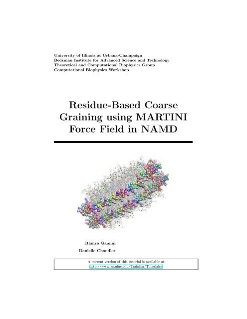
Residue-Based Coarse Graining using MARTINI Force Field in NAMD
Residue-Based Coarse Graining using MARTINI Force Field in NAMD
Residue-Based Coarse Graining using MARTINI Force Field in NAMD

Create successful ePaper yourself
Turn your PDF publications into a flip-book with our unique Google optimized e-Paper software.
University of Ill<strong>in</strong>ois at Urbana-Champaign<br />
Beckman Institute for Advanced Science and Technology<br />
Theoretical and Computational Biophysics Group<br />
Computational Biophysics Workshop<br />
<strong>Residue</strong>-<strong>Based</strong> <strong>Coarse</strong><br />
<strong>Gra<strong>in</strong><strong>in</strong>g</strong> <strong>us<strong>in</strong>g</strong> <strong>MARTINI</strong><br />
<strong>Force</strong> <strong>Field</strong> <strong>in</strong> <strong>NAMD</strong><br />
Ramya Gam<strong>in</strong>i<br />
Danielle Chandler<br />
A current version of this tutorial is available at<br />
http://www.ks.uiuc.edu/Tra<strong>in</strong><strong>in</strong>g/Tutorials/
CONTENTS 2<br />
Contents<br />
1 <strong>Coarse</strong>-gra<strong>in</strong><strong>in</strong>g an atomic structure 8<br />
1.1 Structural model of lipoprote<strong>in</strong>. . . . . . . . . . . . . . . . . . . . 8<br />
1.2 <strong>Coarse</strong>-gra<strong>in</strong><strong>in</strong>g of a lipoprote<strong>in</strong> structure. . . . . . . . . . . . . . 9<br />
1.3 Solvation and Ionization. . . . . . . . . . . . . . . . . . . . . . . . 12<br />
2 Runn<strong>in</strong>g a coarse-gra<strong>in</strong>ed simulation 17<br />
2.1 Prepar<strong>in</strong>g a configuration file. . . . . . . . . . . . . . . . . . . . . 17<br />
2.2 Simulation outputs. . . . . . . . . . . . . . . . . . . . . . . . . . 18<br />
3 Other examples 20<br />
3.1 Ubiquit<strong>in</strong> . . . . . . . . . . . . . . . . . . . . . . . . . . . . . . . 20<br />
3.2 Lipid Bilayer . . . . . . . . . . . . . . . . . . . . . . . . . . . . . 22<br />
3.3 Membrane Prote<strong>in</strong> . . . . . . . . . . . . . . . . . . . . . . . . . . 23
CONTENTS 3<br />
Introduction<br />
In this session, we will learn about coarse-gra<strong>in</strong>ed (CG) molecular dynamics<br />
(MD) simulations. Atomistic simulations are useful computational tools for<br />
<strong>in</strong>vestigat<strong>in</strong>g biological systems such as prote<strong>in</strong>s, lipids and nucleic acids over<br />
timescales of nanoseconds. However, many <strong>in</strong>terest<strong>in</strong>g phenomena, <strong>in</strong>clud<strong>in</strong>g<br />
vesicle fusion, membrane deformation, prote<strong>in</strong>-prote<strong>in</strong> assembly etc., occur at<br />
longer time scales that fall outside the capabilities of atomic scale simulations.<br />
In order to reach the relevant timescales, simplification of the model is required.<br />
The term ”coarse gra<strong>in</strong><strong>in</strong>g” (CG) can be used to refer to any simulation technique<br />
that simplifies the system by group<strong>in</strong>g several atoms of it <strong>in</strong>to one component,<br />
thus to consist of fewer, larger components. CG thereby represents an<br />
attractive alternative to atomistic scale simulations s<strong>in</strong>ce the reduction <strong>in</strong> <strong>in</strong>teraction<br />
particles and number of degrees of freedom allow for simulations to be<br />
run over relatively long periods of time and length scales at a reduced level of<br />
detail.<br />
This tutorial presents one CG method, termed residue-based coarse-gra<strong>in</strong>ed<br />
(RBCG). In a residue-based coarse-gra<strong>in</strong>ed (RBCG) model for biological systems<br />
compris<strong>in</strong>g prote<strong>in</strong>s and or lipids, several atoms are grouped together <strong>in</strong> a<br />
”virtual” bead that <strong>in</strong>teracts through an effective potential. For example, each<br />
am<strong>in</strong>o acid residue and 4 water molecules are represented by 2-5 beads and 1<br />
bead respectively (Figure 1).The reduction of the number of degrees of freedom<br />
and the use of shorter-range potential functions makes the model computationally<br />
very efficient, allow<strong>in</strong>g a <strong>in</strong>crease <strong>in</strong> the base time-step and thus a reduction<br />
of the simulation time by 2 - 3 orders of magnitude compared to the traditional<br />
atomistic models. RBCG MD simulations were performed <strong>in</strong> <strong>NAMD</strong><strong>us<strong>in</strong>g</strong> the<br />
<strong>MARTINI</strong> CG force field developed and parametrized by the group of Siewert<br />
Marr<strong>in</strong>k for use with GROMACS. For the implemented CG force field <strong>in</strong> <strong>NAMD</strong><br />
to be functional, <strong>in</strong> order to reproduce the results of GROMACS, we adapted<br />
the GROMACS switch<strong>in</strong>g function for LJ potential and a shift<strong>in</strong>g function for<br />
Colomb potential only for use of CG simulations.<br />
The tutorial <strong>in</strong>troduces tools for RBCG model<strong>in</strong>g that are provided <strong>in</strong> VMD<br />
as plug<strong>in</strong>s (http://www.ks.uiuc.edu/Research/vmd/plug<strong>in</strong>s/cgtools/).<br />
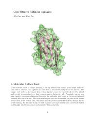
For exercises, we will model prote<strong>in</strong>-lipid assemblies called high-density lipoprote<strong>in</strong>s<br />
(HDL) (Shih et al., J. Str. Biol., 157:579, 2007). HDL are known to function<br />
as cholesterol transporters, facilitat<strong>in</strong>g the removal of excess cholesterol<br />
from the body. Due to the heterogenity of native HDL particles, the details of<br />
how these prote<strong>in</strong>-lipid particles form and the structure they assume <strong>in</strong> their<br />
lipid associated states are not well characterized. <strong>Coarse</strong>-gra<strong>in</strong>ed (CG) molecular<br />
dynamics allows for long-time scale simulations needed to reveal the stable<br />
conformations and also self-assembly of discoidal HDL particles from disordered<br />
prote<strong>in</strong>-lipid complexes. In this tutorial we focus on model<strong>in</strong>g a RBCG structure<br />
of discoidal HDL start<strong>in</strong>g from all-atom for perform<strong>in</strong>g simulations to reveal the<br />
stablity of the widely accepted double-belt model.
CONTENTS 4<br />
Figure 1: Mapp<strong>in</strong>g all-atom to coarse-gra<strong>in</strong>ed structure . Left, am<strong>in</strong>o acid residues and lipid<br />
shown <strong>in</strong> all-atom representation. Right, a coarse-gra<strong>in</strong>ed representation of the same.<br />
To perform simulations <strong>us<strong>in</strong>g</strong> the RBCG representation, one uses VMD and<br />
<strong>NAMD</strong> without any changes <strong>in</strong> comparison with the all-atom case, and work<br />
with the same file types as for all-atom model<strong>in</strong>g, such as PSF and PDB for<br />
structures, and topology, parameter, and configuration files for runn<strong>in</strong>g simulations<br />
(see VMD and <strong>NAMD</strong> tutorials, http://www.ks.uiuc.edu/Tra<strong>in</strong><strong>in</strong>g/Tutorials/).<br />
However, the RBCG PSF, PDB files first need to be created accord<strong>in</strong>g to the<br />
all-atom model that one desires to coarse-gra<strong>in</strong>. In this tutorial, we will learn<br />
how to use the RBCG plug<strong>in</strong>s of VMD to build such files for simulations.
CONTENTS 5<br />
Required Programs<br />
The follow<strong>in</strong>g programs are required for this tutorial:<br />
• VMD: The tutorial assumes that you already have a work<strong>in</strong>g knowledge<br />
of VMD, which is available at http://www.ks.uiuc.edu/Research/vmd/<br />
(for all platforms). The VMD tutorial is available at<br />
http://www.ks.uiuc.edu/Tra<strong>in</strong><strong>in</strong>g/Tutorials/vmd/tutorial-html/<br />
• <strong>NAMD</strong> ”Nightly build May 31, 2012 or later (L<strong>in</strong>ux only)” or<br />
<strong>NAMD</strong> version 2.10 (for all platforms when available): In order to<br />
perform simulations with the CG model <strong>in</strong> this tutorial, <strong>NAMD</strong> should be<br />
correctly <strong>in</strong>stalled on your computer. For <strong>in</strong>stallation <strong>in</strong>structions, please<br />
refer to the <strong>NAMD</strong> Users’ Guide. The <strong>NAMD</strong> tutorial is available <strong>in</strong> both<br />
Unix/MacOSX and W<strong>in</strong>dows versions:<br />
http://www.ks.uiuc.edu/Tra<strong>in</strong><strong>in</strong>g/Tutorials/namd/namd-tutorial-unix-html/<br />
http://www.ks.uiuc.edu/Tra<strong>in</strong><strong>in</strong>g/Tutorials/namd/namd-tutorial-w<strong>in</strong>-html/<br />
Most of the exercises <strong>in</strong> the tutorial are performed <strong>us<strong>in</strong>g</strong> <strong>Residue</strong>-<strong>Based</strong><br />
<strong>Coarse</strong>-<strong>Gra<strong>in</strong><strong>in</strong>g</strong> (RBCG) Tools <strong>in</strong> VMD. The Tools are implemented as a set<br />
of plug<strong>in</strong>s available with their Graphical User Interfaces (GUIs) through VMD<br />
menu:<br />
Extensions → Model<strong>in</strong>g → CG Builder
CONTENTS 6<br />
Figure 2: Ma<strong>in</strong> Graphical User Interface for the CG Builder Tools <strong>in</strong> VMD. Available are<br />
several tools for two CG models, one of which is the RBCG model addressed <strong>in</strong> this tutorial.
CONTENTS 7<br />
Gett<strong>in</strong>g Started<br />
If you downloaded the tutorial from the web you will also need to download the<br />
appropriate files, unzip them, and place them <strong>in</strong> a directory of your choos<strong>in</strong>g.<br />
You should then navigate to that directory as described below. The files for<br />
this tutorial are available at<br />
http://www.ks.uiuc.edu/Tra<strong>in</strong><strong>in</strong>g/Tutorials/<br />
• Unix/Mac OS X Users: In a Term<strong>in</strong>al w<strong>in</strong>dow type:<br />
cd <br />
You can list the content of this directory by <strong>us<strong>in</strong>g</strong> the command ls.<br />
• W<strong>in</strong>dows Users: Navigate to the rbcg-mart<strong>in</strong>i-tutorial → files<br />
directory <strong>us<strong>in</strong>g</strong> W<strong>in</strong>dows Explorer.<br />
You can f<strong>in</strong>d the files for this tutorial <strong>in</strong> the rbcg-mart<strong>in</strong>i-tutorial/files.<br />
Below you can see <strong>in</strong> Fig. 3, the organization of files and directories of rbcg-mart<strong>in</strong>i-tutorial/files/<br />
.<br />
rbcg-mart<strong>in</strong>i-tutorial/les<br />
01-build-cg-model 02-solvate-ionize 03-simulations 04-cgc-top-par-les 05-scripts<br />
01-AA-lipoprote<strong>in</strong>.psf<br />
01-AA-lipoprote<strong>in</strong>.pdb example-output<br />
example-output<br />
cg-waterbox<br />
system-m<strong>in</strong>.conf<br />
system-npt-01.conf<br />
example-output<br />
mart<strong>in</strong>i-cgc<br />
mart<strong>in</strong>i-top<br />
mart<strong>in</strong>i-par<br />
x_mart<strong>in</strong>i_psf.tcl<br />
cg-ionize.tcl<br />
solvate.tcl<br />
dsspcmbi<br />
orient<br />
Figure 3: Directory Structure for tutorial exercises. Sample output for each exercise is<br />
provided <strong>in</strong> an “example-output” subdirectory with<strong>in</strong> each folder.<br />
To start VMD type vmd <strong>in</strong> a Unix term<strong>in</strong>al w<strong>in</strong>dow. Double-click on the VMD<br />
application icon likely located <strong>in</strong> the Applications folder <strong>in</strong> Mac OS X, or click<br />
on the Start → Programs → VMD menu item <strong>in</strong> W<strong>in</strong>dows.<br />
la1.0<br />
06-OtherExamples<br />
Ubiquit<strong>in</strong><br />
POPC<br />
M2-Channel
1 COARSE-GRAINING AN ATOMIC STRUCTURE 8<br />
1 <strong>Coarse</strong>-gra<strong>in</strong><strong>in</strong>g an atomic structure<br />
In this unit you will build the PDB and PSF required for simulation of the<br />
lipoprote<strong>in</strong> assembly, learn<strong>in</strong>g how to take a raw all-atom structure and build a<br />
RBCG system out of it.<br />
1.1 Structural model of lipoprote<strong>in</strong>.<br />
High-density lipoprote<strong>in</strong>s (HDL) are prote<strong>in</strong>-lipid particles, which circulate <strong>in</strong><br />
the blood collect<strong>in</strong>g cholesterol. Apolipoprote<strong>in</strong> A-I (apo A-I), the primary<br />
prote<strong>in</strong> component of HDL, is a 243 residue amphipathic prote<strong>in</strong> conta<strong>in</strong><strong>in</strong>g an<br />
N-term<strong>in</strong>al globular doma<strong>in</strong> and a C-term<strong>in</strong>al lipid b<strong>in</strong>d<strong>in</strong>g doma<strong>in</strong>. The lipid<br />
b<strong>in</strong>d<strong>in</strong>g doma<strong>in</strong> comprises 200 residues, however, the first 11 to 22 residues of the<br />
doma<strong>in</strong> are known not to be <strong>in</strong>volved <strong>in</strong> b<strong>in</strong>d<strong>in</strong>g of lipids <strong>in</strong> the discoidal shaped<br />
HDL particles. Due to heterogenity of HDL particles, high resolution structures<br />
have been difficult to obta<strong>in</strong>. Nanodiscs are nanometer-sized discoidal HDL<br />
that are be<strong>in</strong>g developed as a platform for study<strong>in</strong>g membrane prote<strong>in</strong>s. The<br />
scaffold prote<strong>in</strong> that were used to surround nanodiscs (MSP1) were eng<strong>in</strong>eered<br />
to conta<strong>in</strong> the lipid b<strong>in</strong>d<strong>in</strong>g doma<strong>in</strong> of 200 residues. In this tutorial, we model<br />
a truncated discoidal HDL compris<strong>in</strong>g a truncated lipid b<strong>in</strong>d<strong>in</strong>g doma<strong>in</strong> of apo<br />
A-I (MSP1 ∆(1-11) consist<strong>in</strong>g of 189 residues by delet<strong>in</strong>g the first 11 residues<br />
surround<strong>in</strong>g a lipid core consist<strong>in</strong>g of 160 DPPC lipids. We employ RBCG VMD<br />
plug<strong>in</strong> to model this lipoprote<strong>in</strong> system.<br />
Figure 4: The discoidal HDL nanodisc shown <strong>in</strong> side (left) and top (right) view. The two<br />
monomers of the apo A-I lipid b<strong>in</strong>d<strong>in</strong>g doma<strong>in</strong> are shown <strong>in</strong> violet and cyan. DPPC lipids<br />
are shown tan with lipid head groups <strong>in</strong> yellow.<br />
Provided for you is the all-atom PDB/PSF nanodisc structure with truncated<br />
apo A-I (MSP1 ∆(1-11)) (see Shih et al., J. Str. Biol., 157:579, 2007).<br />
To beg<strong>in</strong>, you will build an all-atom PDB/PSF pair for the PDB structure of<br />
<strong>in</strong>terest. This can be done <strong>us<strong>in</strong>g</strong> a PSFgen script or employ<strong>in</strong>g AutoPSF plug<strong>in</strong><br />
<strong>in</strong> VMD. We assume that the reader is familiar with construct<strong>in</strong>g a PSF<br />
from PDB. Such PDB and PSF are already created: see 01-AA-lipoprotien,<br />
01-AA-lipoprote<strong>in</strong>.psf <strong>in</strong> the directory 01-build-cg-model/.
1 COARSE-GRAINING AN ATOMIC STRUCTURE 9<br />
Navigate to the directory 01-build-cg-model/. You can exam<strong>in</strong>e the segments<br />
of the truncated lipid b<strong>in</strong>d<strong>in</strong>g doma<strong>in</strong> of the apo A-I (MSP1 ∆(1-11) <strong>in</strong><br />
VMD (files 01-AA-lipoprote<strong>in</strong>.pdb and 01-AA-lipoprote<strong>in</strong>.psf <strong>in</strong> 1-build-cg-model/).<br />
One monomer is designated as segname P1, and the other as segname P2. The<br />
DPPC lipid patch is designated as resname DPPC.<br />
1.2 <strong>Coarse</strong>-gra<strong>in</strong><strong>in</strong>g of a lipoprote<strong>in</strong> structure.<br />
Let us now coarse-gra<strong>in</strong> the all-atom lipoprote<strong>in</strong> structure .<br />
1. Start VMD and load the all-atom lipoprote<strong>in</strong> structure (load 01-AA-lipoprote<strong>in</strong>.psf<br />
and 01-AA-lipoprote<strong>in</strong>.pdb <strong>in</strong>to the same molecule).<br />
2. Open the CG Builder <strong>in</strong> VMD (Extensions → Model<strong>in</strong>g → CG Builder),<br />
and choose the option “Create RBCG Model”and hit the button Next->. This<br />
will br<strong>in</strong>g you to the RBCG Builder GUI (Fig. 5).<br />
Figure 5: RBCG Builder GUI.<br />
3. The first step <strong>in</strong> creat<strong>in</strong>g a coarse-gra<strong>in</strong>ed model is to split the system<br />
<strong>in</strong>to appropriate atom clusters and assign the correct bead types to them.<br />
The def<strong>in</strong>itions of the atom clusters are provided <strong>in</strong> the .cgc files <strong>in</strong> the folder<br />
04-cgc-top-par-files/mart<strong>in</strong>i-cgc/. To model our lipoprote<strong>in</strong> system, choose<br />
the User Def<strong>in</strong>ed option to browse and add mart<strong>in</strong>i-lipids.cgc and mart<strong>in</strong>i-prote<strong>in</strong>.cgc.<br />
Note: The options Prote<strong>in</strong>s and Water are set to use old RBCG parameters.
1 COARSE-GRAINING AN ATOMIC STRUCTURE 10<br />
CGC entries. Open one of the .cgc files (i.e.<br />
mart<strong>in</strong>i-prote<strong>in</strong>.cgc), you will see entries of the form<br />
CGBEGIN<br />
(RESNAME) (BEADNAME) 0<br />
(RESNAME) (ATOMNAME) 0 (the first atom should be what you consider<br />
the “central” atom of the cluster)<br />
(RESNAME) (ATOMNAME) 0 (beyond that, the order<strong>in</strong>g is unimportant)<br />
...<br />
CGEND<br />
each of which def<strong>in</strong>es one bead assignment.<br />
An annotated section of the standard CHARMM .top file is<br />
provided for illustrative purposes <strong>in</strong> Appendix A, show<strong>in</strong>g the cgc<br />
bead assignments for all prote<strong>in</strong> residues and for POPE lipids.<br />
4. The ma<strong>in</strong> result of runn<strong>in</strong>g the algorithm is the production of output files<br />
that are written on the hard drive, namely the RBCG PDB and RCG files.<br />
If you want to have specific names for those files, they can be changed <strong>in</strong><br />
the RBCG Builder GUI before hitt<strong>in</strong>g “Build <strong>Coarse</strong> Gra<strong>in</strong> Model” button.<br />
Here, the default filename for PDB/RCG cg-01-AA-lipoprote<strong>in</strong> is changed to<br />
01-CG-lipoprote<strong>in</strong>.<br />
5. Hit the “Build <strong>Coarse</strong> Gra<strong>in</strong> Model” button. Completion of the RBCG<br />
algorithm will take a few moments.<br />
6. The output PDB file conta<strong>in</strong><strong>in</strong>g the newly constructed RBCG model is automatically<br />
loaded <strong>in</strong> VMD as a new molecule, overlapped with the orig<strong>in</strong>al<br />
all-atom model. In case someth<strong>in</strong>g fails, we have provided the output files generated<br />
<strong>in</strong> this step 01-CG-lipoprote<strong>in</strong>.pdb and 01-CG-lipoprote<strong>in</strong>.rcg <strong>in</strong><br />
the 01-build-cg-model/example-output/ folder.<br />
7. The RBCG output PDB file determ<strong>in</strong>es the structure of the coarse-gra<strong>in</strong>ed<br />
lipoprote<strong>in</strong> model. To obta<strong>in</strong> the complete structure for display <strong>in</strong> VMD, or<br />
for subsequent simulations, we need to make a PSF file for the PDB. This<br />
can be done the same way as commonly achieved for all-atom files, namely,<br />
<strong>us<strong>in</strong>g</strong> a PSFgen script or by employ<strong>in</strong>g the AutoPSF VMD plug<strong>in</strong>. Start<br />
VMD and load the cg-lipoprote<strong>in</strong> structure (load 01-CG-lipoprote<strong>in</strong>.pdb).<br />
To employ the AutoPSF plug<strong>in</strong> (Extensions → Model<strong>in</strong>g → Automatic PSF<br />
Builder), remember to delete the default topology file from the list of topologies<br />
<strong>in</strong> the plug<strong>in</strong>, and add the CG topology files (mart<strong>in</strong>i-prote<strong>in</strong>.top and<br />
mart<strong>in</strong>i-lipids.top) located <strong>in</strong> the 04-cgc-top-par-files/mart<strong>in</strong>i-top/<br />
directory. One caveat to keep <strong>in</strong> m<strong>in</strong>d is to ensure you do not generate angles<br />
and dihedrals which are not def<strong>in</strong>ed <strong>in</strong> <strong>MARTINI</strong>. If you are <strong>us<strong>in</strong>g</strong> AutoPSF<br />
plug<strong>in</strong>, uncheck “Regenerate angles/dihedrals” under Options. Click
1 COARSE-GRAINING AN ATOMIC STRUCTURE 11<br />
“Guess and split cha<strong>in</strong>s <strong>us<strong>in</strong>g</strong> current selections”. Note that <strong>in</strong> the Segments<br />
Identified the NTER, CTER patches listed are not def<strong>in</strong>ed for RBCG <strong>in</strong><br />
AutoPSF VMD plug<strong>in</strong>, therefore, we select each cha<strong>in</strong> and hit “Edit Cha<strong>in</strong>”<br />
to change the N term<strong>in</strong>al patch and C term<strong>in</strong>al patch to “NONE”. Once the<br />
patches are changed, hit “Create cha<strong>in</strong>s”. This will create a prelim<strong>in</strong>ary<br />
PSF file 01-CG-lipoprote<strong>in</strong> autopsf.psf and the correspond<strong>in</strong>g PDB file<br />
01-CG-lipoprote<strong>in</strong> autopsf.psf for your coarse-gra<strong>in</strong>ed system.<br />
<strong>MARTINI</strong> mapp<strong>in</strong>g for prote<strong>in</strong> and lipids . In the <strong>MARTINI</strong><br />
model, each prote<strong>in</strong> residue is represented by a “backbone bead”<br />
and one or more “sidecha<strong>in</strong> beads” (with the exception of ALA and<br />
GLY, which are modeled solely by a backbone bead). R<strong>in</strong>g-shaped<br />
sidecha<strong>in</strong>s (TRP, PHE, TYR, HIS) are treated <strong>in</strong> more detail, and<br />
conta<strong>in</strong> 3-4 lighter sidecha<strong>in</strong> beads. Fig. 1 shows three examples of<br />
coarse-gra<strong>in</strong>ed residues. The type of bead to be assigned to each<br />
cluster of atoms is def<strong>in</strong>ed by the non-bonded <strong>in</strong>teractions of that<br />
bead. There are four classes of beads: Q (charged), P (polar), N<br />
(nonpolar) and C (apolar), each with several subtypes. Q and N<br />
types have four subtypes, Qda, Qd, Qa, Q0 and Nda, Nd, Na, N0<br />
which dist<strong>in</strong>guish between the hydrogen-bond<strong>in</strong>g capabilities of the<br />
atom cluster (da = donor or acceptor, d = donor, a = acceptor, 0<br />
= no hydrogen bond<strong>in</strong>g). P and C types have five subtypes, P1,<br />
P2, P3, P4, P5 and C1, C2, C3, C4, C5, where<strong>in</strong> the subscripts 1-5<br />
<strong>in</strong>dicate <strong>in</strong>creas<strong>in</strong>g polar aff<strong>in</strong>ity. By convention, each bead has a<br />
mass of 72 amu. In addition to these “heavy” beads, there is also a<br />
class of light beads with mass 45 amu, used to describe r<strong>in</strong>g shaped<br />
residues. These beads are <strong>in</strong>dicated with a prepended “S”, e.g. SP1,<br />
SC3, SQda, etc. In addition to their lighter mass, they are assigned<br />
a smaller vdW radius and the vdW <strong>in</strong>teraction strength is scaled<br />
by 75%. To be clear, the mass of a bead <strong>in</strong> <strong>MARTINI</strong> is 72 (or<br />
45) amu regardless of whether the masses of the atoms compris<strong>in</strong>g<br />
that bead actually sum to 72. The model<strong>in</strong>g of lipid molecules is<br />
similar to that of prote<strong>in</strong>s, except that the “small” bead types and<br />
secondary structure assignments are not needed. See aga<strong>in</strong> Fig. 1<br />
for a depiction of a lipid <strong>in</strong> coarse-gra<strong>in</strong>ed representation.<br />
8. Correction for prote<strong>in</strong> segments. The next step is to correct the coarsegra<strong>in</strong>ed<br />
PSF file so that the bead types reflect the secondary structure of the<br />
prote<strong>in</strong>. A PSFgen script is provided: fix mart<strong>in</strong>i psf.tcl <strong>in</strong> the folder<br />
05-scripts for this purpose. Open the script to see how this is done. The<br />
script also allows you to choose for charged/uncharged N and C term<strong>in</strong>al.<br />
Copy the script to current work<strong>in</strong>g directory 01-build-cg-model. Also copy<br />
mart<strong>in</strong>i-prote<strong>in</strong>.top. Start VMD and load the “all-atom-lipoprote<strong>in</strong> structure”<br />
(01-AA-lipoprote<strong>in</strong>.psf 01-AA-lipoprote<strong>in</strong>.pdb). Make sure this is<br />
the top molecule. And run the follow<strong>in</strong>g command <strong>in</strong> the VMD Tk Console:<br />
source fix mart<strong>in</strong>i psf.tcl<br />
fix mart<strong>in</strong>i psf 0 mart<strong>in</strong>i-prote<strong>in</strong>.top 01-CG-lipoprote<strong>in</strong> autopsf.psf
1 COARSE-GRAINING AN ATOMIC STRUCTURE 12<br />
01-CG-lipoprote<strong>in</strong> autopsf.pdb CG-fix mart<strong>in</strong>i psf 1 ../05-scripts 1 -1<br />
Note that the script uses the all-atom PSF PDB and RBCG PSF PDB files<br />
you have just created. The first argument here “0” refers to molid of the top<br />
molecule 01-AA-lipoprote<strong>in</strong>.psf and 01-AA-lipoprote<strong>in</strong>.psf. The second<br />
argument is the topology file mart<strong>in</strong>i-prote<strong>in</strong>.top placed <strong>in</strong> the current directory;<br />
if you did not place these files <strong>in</strong> the directory where fix mart<strong>in</strong>i psf.tcl<br />
is located, you will need to specify the correct paths for all the <strong>in</strong>put files while<br />
call<strong>in</strong>g the proc fix mart<strong>in</strong>i psf. The fifth argument “CG-fix mart<strong>in</strong>i psf”<br />
refers to name of the corrected “output PSF/PDB” files. In the sixth argument<br />
we provide the “path” for DSSP secondary structure assignment plug<strong>in</strong><br />
“../05-script”-the default is STRIDE. The last two arguments is for hav<strong>in</strong>g<br />
a positive N term<strong>in</strong>us and negative C term<strong>in</strong>us.<br />
Now open the orig<strong>in</strong>al 01-CG-lipoprote<strong>in</strong> autopsf.psf and the corrected CG-fix mart<strong>in</strong>i psf.psf<br />
PSF files with a text editor. Note that <strong>in</strong> the orig<strong>in</strong>al PSF file, the bacbone<br />
beads (BAS) have generic types (such as P4, P5), whereas <strong>in</strong> the corrected PSF<br />
file, they have been give bead types correspond<strong>in</strong>g to the secondary structure<br />
assignment for each residue.<br />
<strong>MARTINI</strong> mapp<strong>in</strong>g for prote<strong>in</strong> secondary structure . <strong>MARTINI</strong><br />
is sensitive to the secondary structure of the prote<strong>in</strong> it is be<strong>in</strong>g used<br />
to represent. Beads represent<strong>in</strong>g prote<strong>in</strong> backbone are classified<br />
not only by their non-bonded <strong>in</strong>teractions, but on their secondary<br />
structure and the secondary structures of their immediate neighbors.<br />
Backbone beads may be classified as Helix (H), Coil (C),<br />
Extended (E), Turn (T), Bend (B) or Free (F), and the secondary<br />
structure assignment determ<strong>in</strong>es the bonded <strong>in</strong>teractions with neighbor<strong>in</strong>g<br />
backbone beads.<br />
RBCG Builder output files. Sample RBCG Builder output files are provided<br />
<strong>in</strong> the folder 1-build-cg-model/example-output, <strong>in</strong>clud<strong>in</strong>g also the output<br />
files from runn<strong>in</strong>g the AutoPSF and PSFgen script fix mart<strong>in</strong>i psf.tcl.<br />
Note that all these output files are generally go<strong>in</strong>g to be somewhat different<br />
from those you create, due to the probabilistic nature of the RBCG algorithm.<br />
We are almost there! We only have to solvate and ionize the system, then<br />
we can start <strong>us<strong>in</strong>g</strong> the <strong>NAMD</strong> to actually perform a simulation of the RBCG<br />
lipoprote<strong>in</strong> system.<br />
1.3 Solvation and Ionization.<br />
We will now solvate and ionize the system. We will use the VMD’s Solvate<br />
Plug<strong>in</strong>, just as <strong>in</strong> the all-atom case, except that you will use the non-standard<br />
solvent option and place the system <strong>in</strong> a <strong>MARTINI</strong> water box <strong>in</strong> place of the<br />
default.
1 COARSE-GRAINING AN ATOMIC STRUCTURE 13<br />
Figure 6: High-density lipoprote<strong>in</strong> (HDL) nanodisc structure. The two monomers of the<br />
apo A-I lipid b<strong>in</strong>d<strong>in</strong>g doma<strong>in</strong> are shown <strong>in</strong> orange and red and the DPPC lipids are shown<br />
<strong>in</strong> blue with lipid head groups <strong>in</strong> green. The all-atom structure is shown on the left, and an<br />
example of a RBCG structure is shown on the right. Both all-atom and RBCG structures are<br />
shown from the sideview.<br />
1. First, load the files 01-CG-fix mart<strong>in</strong>i psf.psf and 01-CG-fix mart<strong>in</strong>i psf.pdb<br />
<strong>in</strong>to VMD.<br />
<strong>MARTINI</strong> water. Water molecules <strong>in</strong> <strong>MARTINI</strong> are represented by<br />
a s<strong>in</strong>gle bead (of mass 72 amu). To protect aga<strong>in</strong>st the possibility<br />
of the water box “freez<strong>in</strong>g” on very large timescales, a second type<br />
of water molecule is def<strong>in</strong>ed with a slighly larger VdW radius. These<br />
are referred to as “antifreeze particles”, and it is recommended that<br />
10% of the waterbox be antifreeze particles.<br />
2. To use the Solvate plug<strong>in</strong>, select Extensions → Model<strong>in</strong>g → Add Solvation<br />
Box <strong>in</strong> the ma<strong>in</strong> w<strong>in</strong>dow.<br />
3. Set “Boundary”, the m<strong>in</strong>imum distance between water and solute to 5 <strong>in</strong>stead<br />
of the default 2.4.<br />
4. Set “Box Padd<strong>in</strong>g” to 15 angstrom padd<strong>in</strong>g <strong>in</strong> x, y and z directions.<br />
5. Check the “nonstandard solvent” to use the equilibrated CG waterbox. The<br />
PDB/PSF files are provided <strong>in</strong> the folder 02-solvate-ionize/cg-waterbox/<br />
and the TOP file is located <strong>in</strong> the folder /04-cgc-top-par-files/mart<strong>in</strong>i-top.<br />
6. Set “Solvent box side length” to 100. This corresponds to the box side length<br />
of the provided equilibrated CG waterbox.<br />
7. Set “Solvent box key selection” to “name W WAF”. This corresponds to the<br />
water and anti-freeze CG beads.
1 COARSE-GRAINING AN ATOMIC STRUCTURE 14<br />
Figure 7: Solvate plug<strong>in</strong> <strong>in</strong> VMD.<br />
8. Then click Solvate and wait for a m<strong>in</strong>ute or two. The Solvate should<br />
generate the 02-solvate PSF PDB files.<br />
9. To ionize and neutralize the system, we will use the modified version of<br />
autoionize PSFgen script cg-ionize.tcl provided <strong>in</strong> the folder 05-scripts.<br />
Make sure the the output files of Solvate (02-solvate.psf and 02-solvate.pdb)<br />
are currently loaded <strong>in</strong>to VMD.
1 COARSE-GRAINING AN ATOMIC STRUCTURE 15<br />
<strong>MARTINI</strong> ions. Ions are also represented as s<strong>in</strong>gle (charged)<br />
particles of mass 72 amu.<br />
10. Type <strong>in</strong> the Tk Console w<strong>in</strong>dow:<br />
source cg-ionize.tcl<br />
autoionize -psf 02-solvate.psf -pdb 02-solvate.pdb -sc 0.1 -o 02-ionize<br />
The -sc 0.1 option tells autoionize to neutralize and set salt concentration<br />
to 0.1 (mol/L). The default cation is CL and default anion is NA. The option<br />
-cation -anion can be used to specify the cation and anion other than default<br />
ions.<br />
11. Load the output files of autoionize (02-ionize.psf and 02-ionize.pdb)<br />
<strong>in</strong>to VMD and check the ions are really there and the system is neutral.<br />
Type <strong>in</strong> the Tk Console w<strong>in</strong>dow:<br />
set all [atomselect top all]<br />
measure sumweights $all weight charge<br />
You should get:<br />
0.0<br />
F<strong>in</strong>ally, after all this work, we are ready for m<strong>in</strong>imization and equilibration<br />
with <strong>NAMD</strong>. This is described <strong>in</strong> the next unit.
1 COARSE-GRAINING AN ATOMIC STRUCTURE 16<br />
Figure 8: F<strong>in</strong>al simulation system <strong>in</strong>clud<strong>in</strong>g the truncated apo A-I prote<strong>in</strong>, DPPC, water,<br />
and ions.
2 RUNNING A COARSE-GRAINED SIMULATION 17<br />
2 Runn<strong>in</strong>g a coarse-gra<strong>in</strong>ed simulation<br />
We are now almost ready to simulate the system of RBCG lipoprotien assembly.<br />
In this section we will discuss first how to write a <strong>NAMD</strong> configuration file for<br />
an RBCG system. We will then perform the simulation, and discuss the file<br />
outputs and simulation result.<br />
To perform exercises, navigate to the folder 03-simulation/.<br />
2.1 Prepar<strong>in</strong>g a configuration file.<br />
S<strong>in</strong>ce RBCG was designed to be compatible with <strong>NAMD</strong>, an RBCG configuration<br />
file looks similar to a normal, all-atom, <strong>NAMD</strong> configuration file that you<br />
might have used before.<br />
1. A sample configuration file system-npt-01.conf has been prepared for you<br />
<strong>in</strong> the directory example-output/. Copy it to the folder where you want to run<br />
the simulation, and open it with a text editor. Remember to create <strong>in</strong> the same<br />
folder subfolder output and <strong>in</strong>put, and add your CG files to the folder <strong>in</strong>put<br />
analogously to how it is done <strong>in</strong> example-output/. Note that you will need here<br />
RBCG parameter files for CG lipids and prote<strong>in</strong>s, which we have not used before.<br />
The paramter files are located <strong>in</strong> 04-cgc-top-par-files/mart<strong>in</strong>i-par/ folder.<br />
2. The configuration file conta<strong>in</strong>s many options (entries <strong>in</strong> the first column), followed<br />
by their parameters (entries <strong>in</strong> the second column) specifically chosen for<br />
the simulated system. Assum<strong>in</strong>g readers already have experience with <strong>NAMD</strong><br />
simulations, here we will only go through those options that require special adjustments<br />
for an RBCG system. New <strong>NAMD</strong> users are encouraged to consult<br />
the <strong>NAMD</strong> Tutorial and <strong>NAMD</strong> User’s Guide.<br />
3. We <strong>in</strong>troduce a new parameter cosAngles. This is required to allow for the<br />
cos<strong>in</strong>e-based angle potential energy term conventionally used <strong>in</strong> GROMACS, as<br />
opposed to the harmonic angle term used <strong>in</strong> <strong>NAMD</strong>. cosAngles is turned on.<br />
4. In the text editor display<strong>in</strong>g the content of system-npt-01.conf, scroll down<br />
to the section # <strong>Force</strong>-<strong>Field</strong> Parameters. Note all l<strong>in</strong>es beg<strong>in</strong>n<strong>in</strong>g with # are<br />
comments ignored by <strong>NAMD</strong>.<br />
Under # <strong>Force</strong>-<strong>Field</strong> Parameters, you will f<strong>in</strong>d simulation options that<br />
might need different parameters than those of an all-atom simulation. These<br />
options def<strong>in</strong>e how you want the <strong>in</strong>teractions between beads to be computed.<br />
exclude parameter is set 1-2, mart<strong>in</strong>iSwitch<strong>in</strong>g, a new key parameter, is<br />
turned on,PME is turned off and dielectric is set 15.0.<br />
It should be noted that for the use of <strong>MARTINI</strong> force field <strong>in</strong> <strong>NAMD</strong>, a GRO-<br />
MACS switch<strong>in</strong>g function is adapted for LJ potential with switchdist 9.0 and<br />
cutoff 12.0, and a shift<strong>in</strong>g function for Colomb potential with switchdist
2 RUNNING A COARSE-GRAINED SIMULATION 18<br />
0.0 hardcoded <strong>in</strong> the <strong>NAMD</strong> source code and cutoff 12.0 .<br />
5. Scroll down to the section # Integrator Parameters.<br />
The parameter timestep has a value of 20.0, imply<strong>in</strong>g that the <strong>in</strong>tegration<br />
timestep of the simulation is 20 fs/step. A typical all-atom simulation uses 1<br />
or 2 fs/step, hence the RBCG gives a speedup of 20 from the choice of <strong>in</strong>tegration<br />
timestep alone. The choice of the timestep depends on how fast beads<br />
are mov<strong>in</strong>g <strong>in</strong> the simulation, and, thus, the maximal timestep possible (so that<br />
the simulation does not crash) is determ<strong>in</strong>ed by the strength of <strong>in</strong>teractions,<br />
e.g., stiffness of bonds, as mentioned above. If your simulation crashes with a<br />
timestep of 20 fs/step, start<strong>in</strong>g the simulation with a shorter timestep might fix<br />
the problem. Then timestep can be <strong>in</strong>creased when the system becomes stable<br />
later <strong>in</strong> the simulation. For m<strong>in</strong>imization, one can do a larger value for timestep<br />
of 40 fs/step.<br />
6. Constant temperature is ma<strong>in</strong>ta<strong>in</strong>ed <strong>in</strong> this RBCG simulation <strong>us<strong>in</strong>g</strong> Langev<strong>in</strong><br />
dynamics, as usually done <strong>in</strong> all-atom simulations. You can take a look at these<br />
parameters under # Constant Temperature Control. The Langev<strong>in</strong> dynamics<br />
<strong>in</strong>troduces viscous drag and random forces act<strong>in</strong>g on each CG bead, which<br />
can be used to mimic the viscosity of the solvent and the Brownian motion<br />
due to random hits from the molecules of the solvent. A s<strong>in</strong>gle parameter,<br />
langev<strong>in</strong>Damp<strong>in</strong>g, is used to account for these effects. Here, langev<strong>in</strong>Damp<strong>in</strong>g<br />
is set to 1 ps −1 .<br />
7. We will first perform m<strong>in</strong>imization before runn<strong>in</strong>g the simulation <strong>in</strong> NPT.<br />
You can see that the simulation is designed to be m<strong>in</strong>imized by 5000 steps (see<br />
system-m<strong>in</strong>.conf) to elim<strong>in</strong>ate the possible steric clashes, and subsequently run<br />
for 50,000,000 steps. This corresponds to 50,000,000 steps × 20 fs/step = 100 ns<br />
simulation time.<br />
8. Close the text editor display<strong>in</strong>g configuration file. Run the m<strong>in</strong>imization<br />
by typ<strong>in</strong>g namd2 system-m<strong>in</strong>.conf > system-m<strong>in</strong>.log <strong>in</strong> a term<strong>in</strong>al w<strong>in</strong>dow.<br />
This is a short run of m<strong>in</strong>imization for 5000 steps that takes about 5 m<strong>in</strong>utes<br />
to complete. Once this step is complete, run a short simulation for 10,000,000<br />
steps <strong>in</strong> NPT by typ<strong>in</strong>g namd2 system-npt-01.conf > system-npt-01.log<br />
2.2 Simulation outputs.<br />
On a one-processor mach<strong>in</strong>e, a 100 ns simulation will take about two days to<br />
complete, but actually we do not need to run the full simulation. The general<br />
trend is obvious already after about the first 10 ns, which can be achieved with<strong>in</strong><br />
an hour or two. If you do not wish to run the simulation yourself, you can use<br />
the files provided <strong>in</strong> example-output/ for the follow<strong>in</strong>g discussion on file outputs<br />
and results.
2 RUNNING A COARSE-GRAINED SIMULATION 19<br />
1. Open the logfile of the simulation, system-npt-01.log, with a text editor.<br />
If you did not run the simulation, use example-output/system-npt-01.log.<br />
The logfile of a simulation conta<strong>in</strong>s useful <strong>in</strong>formation. When your simulation<br />
crashes, check<strong>in</strong>g the logfile for the error message is the first step of fix<strong>in</strong>g<br />
the problem. The logfile can also give you an estimate on how long a simulation<br />
will run. F<strong>in</strong>d the words “Benchmark time” <strong>in</strong> system-npt-01.log, here you<br />
can f<strong>in</strong>d the speed of the simulation. Now let’s exam<strong>in</strong>e the system via VMD.<br />
2. Close the text editor. Open VMD, and load the psf file of the system,<br />
02-ionize.psf. If you did not run the simulation, make sure you use the provided<br />
example-output/<strong>in</strong>put/02-ionize.psf.<br />
3. Load the output dcd files, system-npt-01.dcd. If you did not run the simulation,<br />
use the one provided example-output/output/system-npt-01.dcd. In<br />
this case, you will have 1000 frames loaded <strong>in</strong> VMD, one frame for 20 picosecond<br />
of the simulation.<br />
Figure 9: Simulation result of the lipoprote<strong>in</strong> system. Left: beg<strong>in</strong>n<strong>in</strong>g of the simulation.<br />
Right: system after 100 ns.<br />
Use VMD to take a look at the simulation result. Throughout the trajectory,<br />
the <strong>in</strong>itial discoidal shape of the MSP1 (1-11) nanodisc is ma<strong>in</strong>ta<strong>in</strong>ed well.<br />
After 100 ns of simulation time, the overall “double-belt” like configuration of
3 OTHER EXAMPLES 20<br />
the two apo A-I strands rema<strong>in</strong>ed <strong>in</strong>tact and stable such that the prote<strong>in</strong> helices<br />
rema<strong>in</strong>ed perpendicular to the lipid tail groups. A full trajectory of 100 ns<br />
is also provided for you example-output/output/system-full5000.dcd. The<br />
prote<strong>in</strong> strands <strong>in</strong> this configuration had neither a gap nor an overlap with the<br />
prote<strong>in</strong> ends just touch<strong>in</strong>g each other. This observation correlates well with<br />
previous all-atom MD simulations and experimental results suggest<strong>in</strong>g that the<br />
first 11 N-term<strong>in</strong>al residues are not needed for the formation of nanodiscs of<br />
this size and composition. A simple RBCG simulation used here demonstrates<br />
very well stability of the double-belt confguration suggest<strong>in</strong>g this an equilibrium<br />
structure of the nanodisc model of HDL. For more <strong>in</strong>formation on assembly of<br />
the lipoprote<strong>in</strong> system, please see Shih et al., J. Str. Biol., 157:579, 2007.<br />
To familarize yourself with the process, you may want to work through several<br />
other examples. Below, we provide three examples which follows the same<br />
procedure as expla<strong>in</strong>ed for the lipoprote<strong>in</strong> case. However, you can simply use<br />
the ready-to-use tcl scripts <strong>in</strong>stead of the GUIs.<br />
3 Other examples<br />
3.1 Ubiquit<strong>in</strong><br />
Directory: 06-OtherExamples/Ubiquit<strong>in</strong><br />
In this section, you will coarse-gra<strong>in</strong> and set up simulation files for ubiquit<strong>in</strong> <strong>in</strong><br />
a water box. Provided for you is 1UBQ.pdb, downloaded from www.rcsb.org,<br />
and several build scripts.<br />
Build<strong>in</strong>g the system (step 0)<br />
The first step is to build an all-atom PDB/PSF pair for 1UBQ.pdb. Do this by<br />
typ<strong>in</strong>g<br />
vmd -dispdev text -e 00-make-AA-psf.tcl > 00-make-AA-psf.log<br />
on the command l<strong>in</strong>e. This will create AA-ubiquit<strong>in</strong>.pdb and AA-ubiquit<strong>in</strong>.psf<br />
<strong>Coarse</strong>-gra<strong>in</strong> your system (step 1)<br />
The next step is to coarse-gra<strong>in</strong> the prote<strong>in</strong>. This is done by 01-coarse-gra<strong>in</strong>.tcl.
3 OTHER EXAMPLES 21<br />
To run this script, type<br />
vmd -dispdev text -e 01-coarse-gra<strong>in</strong>.tcl > 01-coarse-gra<strong>in</strong>.log.<br />
Open the script file with your text editor of choice and <strong>in</strong>spect its contents.<br />
This and all other scripts provided are commented so that you can understand<br />
what each part of the script does.<br />
Create a PSF file (step 2)<br />
Now you will create a prelim<strong>in</strong>ary psf file for your coarse-gra<strong>in</strong>ed system. Do<br />
this with<br />
vmd -dispdev text -e 02a-make-<strong>in</strong>itial-CG-psf.tcl > 02a-make-<strong>in</strong>itial-CG-psf.log<br />
You should now have the files cg-ubiquit<strong>in</strong>.pdb, cg-ubiquit<strong>in</strong>.rcg, cg-ubiquit<strong>in</strong>-<strong>in</strong>it.pdb,<br />
and cg-ubiquit<strong>in</strong>-<strong>in</strong>it.psf.<br />
The next step is to correct the coarse-gra<strong>in</strong>ed psf file so that the bead types<br />
reflect the secondary structure of the prote<strong>in</strong>. To do this, run<br />
vmd -dispdev text -e 02b-correct-CG-psf.tcl > 02b-correct-CG-psf.log<br />
Solvate (step 3)<br />
Now that we have constructed the PDB/PSF pair for the prote<strong>in</strong>, we can construct<br />
a water box around it. To do this, we will use the solvate procedure,<br />
<strong>us<strong>in</strong>g</strong> the <strong>MARTINI</strong> cg-waterbox. Open 03-solvate.tcl with a text editor for<br />
an example of how to do this. Run solvate with<br />
vmd -dispdev text -e 03a-solvate.tcl > 03a-solvate.log.<br />
Next we will run a script to remove any waters too close to the prote<strong>in</strong> that<br />
solvate might have missed, just as we would do for an all-atom system.<br />
vmd -dispdev text -e 03b-remove-waters.tcl > 03b-remove-waters.log.<br />
Ionize (step 4)<br />
Last, we will neutralize the system <strong>us<strong>in</strong>g</strong> a modified version of the autoionize<br />
procedure (provided <strong>in</strong> cgionize.tcl). Copy the mart<strong>in</strong>i-ions.top file to the<br />
current directory. Run<br />
vmd -dispdev text -e 04-ionize.tcl > 04-ionize.log.<br />
You should now have the files ionized.pdb and ionized.psf <strong>in</strong> your directory.<br />
Set up the simulation files (step 5)<br />
Some configuration files have been provided for you: ubiquit<strong>in</strong>-m<strong>in</strong>.conf,<br />
ubiquit<strong>in</strong>-01.conf, and ubiquit<strong>in</strong>-02.conf. A short m<strong>in</strong>imization is done<br />
<strong>in</strong> ubiquit<strong>in</strong>-m<strong>in</strong>.conf. Equilibration is started <strong>in</strong> ubiquit<strong>in</strong>-01.conf, and
3 OTHER EXAMPLES 22<br />
cont<strong>in</strong>ued <strong>in</strong> ubiquit<strong>in</strong>-02.conf. It will often be necessary to run with a<br />
shorter timestep <strong>in</strong> the first stages of a simulation until the system stablilizes.<br />
This is why the timestep is set to 10 fs <strong>in</strong> ubiquit<strong>in</strong>-01.conf and then <strong>in</strong>creased<br />
to 40 fs <strong>in</strong> ubiquit<strong>in</strong>-02.conf. As a general po<strong>in</strong>t of advice, if you<br />
f<strong>in</strong>d that your simulation crashes frequently with the “atoms mov<strong>in</strong>g too fast”<br />
error, temporarily decreas<strong>in</strong>g the timestep may solve the problem.<br />
Run the simulation (step 6)<br />
This system is small enough to run on your desktop/laptop, so try runn<strong>in</strong>g the<br />
simulations and open the trajectory <strong>in</strong> VMD.<br />
3.2 Lipid Bilayer<br />
Directory: 06-OtherExamples/POPC<br />
In this section, you will coarse-gra<strong>in</strong> and set up simulation files for a system<br />
conta<strong>in</strong><strong>in</strong>g a membrane patch.<br />
You are provided with a small all-atom POPC membrane patch, and several<br />
build scripts.<br />
<strong>Coarse</strong>-gra<strong>in</strong> your system (step 1)<br />
The first step is to coarse-gra<strong>in</strong> the lipid patch and build a coarse-gra<strong>in</strong>ed<br />
PDB/PSF pair. Do this by runn<strong>in</strong>g<br />
vmd -dispdev text -e 01-coarse-gra<strong>in</strong>.tcl > 01-coarse-gra<strong>in</strong>.log,<br />
and open the script <strong>in</strong> a text file to see how this is be<strong>in</strong>g done.<br />
Create a PSF file (step 2)<br />
Create a coarse-gra<strong>in</strong>ed PDB/PDF pair for your system <strong>us<strong>in</strong>g</strong><br />
vmd -dispdev text -e 02-make-CG-psf.tcl > 02-make-CG-psf.log,
3 OTHER EXAMPLES 23<br />
Unlike <strong>in</strong> the ubiquit<strong>in</strong> example, the psf file requires no further correction because<br />
this system conta<strong>in</strong>s no prote<strong>in</strong> segments.<br />
Solvate (step 3)<br />
Now we will add a water box, aga<strong>in</strong> <strong>us<strong>in</strong>g</strong> solvate with the provided <strong>MARTINI</strong><br />
files. Do this by runn<strong>in</strong>g<br />
vmd -dispdev text -e 03a-solvate.tcl > 03a-solvate.log.<br />
Next we will run a script to remove any waters that may have ended up <strong>in</strong><br />
the hydrophobic region on the outside of the membrane patch, aga<strong>in</strong> just as we<br />
would do for an all-atom system.<br />
vmd -dispdev text -e 03b-remove-waters.tcl > 03b-remove-waters.log.<br />
Ionize (step 4)<br />
F<strong>in</strong>ally, we will neutralize the system, aga<strong>in</strong> <strong>us<strong>in</strong>g</strong> the modified version of autoionize.<br />
Make sure, you copy the mart<strong>in</strong>i-ions.top to the current directory.<br />
And, run<br />
vmd -dispdev text -e 04-ionize.tcl > 04-ionize.log.<br />
Set up the simulation files (step 5)<br />
Aga<strong>in</strong>, several configuration files (popcpatch-m<strong>in</strong>.conf, popcpatch-01.conf,<br />
popcpatch-02.conf) have been provided for you. Note that s<strong>in</strong>ce this is a<br />
membrane simulation useFlexibleCell should be turned on.<br />
Run the simulation (step 6)<br />
Aga<strong>in</strong>, the system should be small enough to run on one processor!<br />
3.3 Membrane Prote<strong>in</strong>
3 OTHER EXAMPLES 24<br />
Directory: 06-OtherExamples/M2-channel<br />
In this section, you will coarse-gra<strong>in</strong> and set up simulation files for a membrane<br />
prote<strong>in</strong> system, conta<strong>in</strong><strong>in</strong>g both prote<strong>in</strong> and lipid segments. The prote<strong>in</strong><br />
used <strong>in</strong> this section is the M2 proton channel (2RLF.pdb), which is composed<br />
of several non-covalently-bound homo-oliomers. Therefore, this example will<br />
demonstrate not only how to comb<strong>in</strong>e lipids and prote<strong>in</strong>, but how to handle<br />
modular prote<strong>in</strong>s <strong>in</strong> <strong>MARTINI</strong>. Please note that M2 was chosen as a proof-ofconcept<br />
example merely because it is small and well known; whether it can be<br />
adequately modeled <strong>in</strong> RBCG representation is another matter. In all-atom<br />
simulations, the oligomers are held together <strong>in</strong> part by hydrogen-bond<strong>in</strong>g <strong>in</strong>teractions,<br />
which are lost <strong>in</strong> the coarse-gra<strong>in</strong><strong>in</strong>g process. To compensate, you<br />
must use the extraBonds feature of <strong>NAMD</strong> to add extra constra<strong>in</strong>ts to keep<br />
the oligomers together.<br />
Create all-atom PDB and PSF files (step 0)<br />
As <strong>in</strong> the ubiquit<strong>in</strong> case, we must first construct an all-atom PDB/PSF file pair<br />
for the prote<strong>in</strong> <strong>us<strong>in</strong>g</strong> a PDB file downloaded from www.rcsb.org databse. The<br />
first script (00-make-AA-psf.tcl) replicates the prote<strong>in</strong> from 2RLF, assembles<br />
the oligomer, and aligns it along the z-axis. To do this, simply run<br />
vmd -dispdev text -e 00a-make-AA-psf.tcl > 00a-make-AA-psf.log.<br />
Open the script file if you are <strong>in</strong>terested <strong>in</strong> see<strong>in</strong>g how this is done.<br />
Now, s<strong>in</strong>ce this is a membrane simulation, the next th<strong>in</strong>g to do is to comb<strong>in</strong>e<br />
it with the membrane. First run<br />
vmd -dispdev text -e 00b-comb<strong>in</strong>e-with-lipids.tcl > 00b-comb<strong>in</strong>e-with-lipids.log.<br />
<strong>Coarse</strong>-gra<strong>in</strong> your system (step 1)<br />
Now we coarse-gra<strong>in</strong> the system:<br />
vmd -dispdev text -e 01-coarse-gra<strong>in</strong>.tcl > 01-coarse-gra<strong>in</strong>.log,<br />
Create a PSF file (step 2)<br />
Create a prelim<strong>in</strong>ary PSF file with:<br />
vmd -dispdev text -e 02a-make-<strong>in</strong>itial-CG-psf.tcl > 02a-make-<strong>in</strong>itial-CG-psf.log<br />
S<strong>in</strong>ce this system conta<strong>in</strong>s both lipid and prote<strong>in</strong> segments, we will need to correct<br />
the psf file to account for secondary structure:<br />
vmd -dispdev text -e 02b-correct-CG-psf.tcl > 02b-correct-CG-psf.log<br />
Solvate and Ionize (steps 3 and 4)<br />
Now we solvate, remove unwanted waters, and ionize the system, just as before
3 OTHER EXAMPLES 25<br />
(Note: Copy the mart<strong>in</strong>i-ions.top file to the current directory):<br />
vmd -dispdev text -e 03a-solvate.tcl > 03a-solvate.log<br />
vmd -dispdev text -e 03b-remove-waters.tcl > 03b-remove-waters.log<br />
vmd -dispdev text -e 04-ionize.tcl > 04-ionize.log.<br />
Set up the simulation files (step 5)<br />
Usually for a membrane prote<strong>in</strong> (prote<strong>in</strong> embedded <strong>in</strong> membrane), one beg<strong>in</strong>s<br />
the simulation with the prote<strong>in</strong> held <strong>in</strong> place, to let the lipids relax around the<br />
prote<strong>in</strong>. For more <strong>in</strong>formation, refer to the Membrane Prote<strong>in</strong> tutorial. We do<br />
this with <strong>NAMD</strong>’s constra<strong>in</strong>ts option, and create the necessary constra<strong>in</strong>t file<br />
here:<br />
vmd -dispdev text -e 05a-make-constra<strong>in</strong>ts.tcl > 05a-make-constra<strong>in</strong>ts.log.<br />
Last, s<strong>in</strong>ce our prote<strong>in</strong> conta<strong>in</strong>s several non-covalently-bonded segments, we<br />
must use <strong>NAMD</strong>’s extrabonds feature to keep the prote<strong>in</strong> from fall<strong>in</strong>g apart.<br />
This script shows an example of how to construct such a file:<br />
vmd -dispdev text -e 05b-make-extrabonds.tcl > 05b-make-extrabonds.log.<br />
If you are aware of particular <strong>in</strong>teractions between monomers, it makes sense<br />
to represent those as extraBonds. Beyond that, the choice of extraBonds is<br />
a matter of trial-and-error. You must use your own judgement as to whether<br />
or not the extraBonded structure adequately represents your oligomeric prote<strong>in</strong>.<br />
Run the simulation (step 6)<br />
This system is slightly larger than the first two, but should still be manageable<br />
on your desktop/laptop. So try runn<strong>in</strong>g the simulation and open the trajectory<br />
<strong>in</strong> VMD.<br />
This ends the RBCG tutorial. You are now ready to use RBCG!<br />
Acknowledgement:<br />
Development of this tutorial was supported by the National Institutes of Health<br />
(P41-RR005969 - Resource for Macromolecular Model<strong>in</strong>g and Bio<strong>in</strong>formatics).
Appendix<br />
This appendix is essentially a visual representation of the <strong>in</strong>formation encoded <strong>in</strong> the coarse-gra<strong>in</strong><br />
.cgc files, show<strong>in</strong>g how each of the am<strong>in</strong>o acids as well as a POPC lipid is divided <strong>in</strong>to coarsegra<strong>in</strong>ed<br />
beads. Excerpts from the standard CHARMM topology file are shown with the Mart<strong>in</strong>i<br />
bead assignments overlaid.<br />
1
RESI ALA 0.00<br />
GROUP<br />
ATOM N NH1 -0.47 ! |<br />
ATOM HN H 0.31 ! HN-N<br />
ATOM CA CT1 0.07 ! | HB1<br />
ATOM HA HB 0.09 ! | /<br />
GROUP ! HA-CA--CB-HB2<br />
ATOM CB CT3 -0.27 ! | \<br />
ATOM HB1 HA 0.09 ! | HB3<br />
ATOM HB2 HA 0.09 ! O=C<br />
ATOM HB3 HA 0.09 ! |<br />
GROUP !<br />
ATOM C C 0.51 BAS = P4<br />
ATOM O O -0.51<br />
BOND CB CA N HN N CA<br />
BOND C CA C +N CA HA CB HB1 CB HB2 CB HB3<br />
DOUBLE O C<br />
RESI ARG 1.00<br />
GROUP<br />
ATOM N NH1 -0.47 ! | SI1 = N0r HH11<br />
ATOM HN H 0.31 ! HN-N |<br />
ATOM CA CT1 0.07 ! | HB1 HG1 HD1 HE NH1-HH12<br />
ATOM HA HB 0.09 ! | | | | | //(+)<br />
GROUP ! HA-CA--CB--CG--CD--NE--CZ<br />
ATOM CB CT2 -0.18 ! | | | | \<br />
ATOM HB1 HA 0.09 ! | HB2 HG2 HD2 NH2-HH22<br />
ATOM HB2 HA 0.09 ! O=C |<br />
GROUP ! | HH21<br />
ATOM CG CT2 -0.18<br />
ATOM HG1 HA 0.09<br />
ATOM HG2 HA 0.09<br />
GROUP<br />
ATOM CD CT2 0.20<br />
ATOM HD1 HA 0.09<br />
ATOM HD2 HA 0.09<br />
ATOM NE NC2 -0.70<br />
ATOM HE HC 0.44<br />
ATOM CZ C 0.64<br />
ATOM NH1 NC2 -0.80<br />
ATOM HH11 HC 0.46<br />
ATOM HH12 HC 0.46<br />
ATOM NH2 NC2 -0.80<br />
ATOM HH21 HC 0.46<br />
ATOM HH22 HC 0.46<br />
GROUP<br />
ATOM C C 0.51<br />
ATOM O O -0.51<br />
BAS = P5<br />
SI2 = Qdr<br />
BOND CB CA CG CB CD CG NE CD CZ NE<br />
BOND NH2 CZ N HN N CA<br />
BOND C CA C +N CA HA CB HB1<br />
BOND CB HB2 CG HG1 CG HG2 CD HD1 CD HD2<br />
BOND NE HE NH1 HH11 NH1 HH12 NH2 HH21 NH2 HH22<br />
DOUBLE O C CZ NH1<br />
RESI ASN 0.00<br />
GROUP<br />
ATOM N NH1 -0.47 ! |<br />
ATOM HN H 0.31 ! HN-N<br />
ATOM CA CT1 0.07 ! | HB1 OD1 HD21 (cis to OD1)<br />
ATOM HA HB 0.09 ! | | || /<br />
GROUP ! HA-CA--CB--CG--ND2<br />
ATOM CB CT2 -0.18 ! | | \<br />
ATOM HB1 HA 0.09 ! | HB2 HD22 (trans to OD1)<br />
ATOM HB2 HA 0.09 ! O=C<br />
GROUP ! |<br />
SID = P5n<br />
ATOM CG CC 0.55<br />
BAS = P5<br />
ATOM OD1 O -0.55<br />
GROUP<br />
ATOM ND2 NH2 -0.62<br />
ATOM HD21 H 0.32<br />
ATOM HD22 H 0.30<br />
GROUP<br />
ATOM C C 0.51<br />
ATOM O O -0.51<br />
BOND CB CA CG CB ND2 CG<br />
BOND N HN N CA C CA C +N<br />
BOND CA HA CB HB1 CB HB2 ND2 HD21 ND2 HD22<br />
DOUBLE C O CG OD1<br />
2<br />
RESI ASP -1.00<br />
GROUP<br />
ATOM N NH1 -0.47 ! | SID = Qad<br />
ATOM HN H 0.31 ! HN-N<br />
ATOM CA CT1 0.07 ! | HB1 OD1<br />
ATOM HA HB 0.09 ! | | //<br />
GROUP ! HA-CA--CB--CG<br />
ATOM CB CT2 -0.28 ! | | \<br />
ATOM HB1 HA 0.09 ! | HB2 OD2(-)<br />
ATOM HB2 HA 0.09 ! O=C<br />
ATOM CG CC 0.62 ! |<br />
ATOM OD1 OC -0.76<br />
ATOM OD2 OC -0.76 BAS = P5<br />
GROUP<br />
ATOM C C 0.51<br />
ATOM O O -0.51<br />
BOND CB CA CG CB OD2 CG<br />
BOND N HN N CA C CA C +N<br />
BOND CA HA CB HB1 CB HB2<br />
DOUBLE O C CG OD1<br />
RESI CYS 0.00<br />
GROUP<br />
ATOM N NH1 -0.47 ! |<br />
ATOM HN H 0.31 ! HN-N SID = C5c<br />
ATOM CA CT1 0.07 ! | HB1<br />
ATOM HA HB 0.09 ! | |<br />
GROUP ! HA-CA--CB--SG<br />
ATOM CB CT2 -0.11 ! | | \<br />
ATOM HB1 HA 0.09 ! | HB2 HG1<br />
ATOM HB2 HA 0.09 ! O=C<br />
ATOM SG S -0.23 ! |<br />
ATOM HG1 HS 0.16<br />
GROUP<br />
BAS = P5<br />
ATOM C C 0.51<br />
ATOM O O -0.51<br />
BOND CB CA SG CB N HN N CA<br />
BOND C CA C +N CA HA CB HB1<br />
BOND CB HB2 SG HG1<br />
DOUBLE O C<br />
RESI GLN 0.00<br />
GROUP<br />
BAS = P5<br />
ATOM N NH1 -0.47 ! |<br />
ATOM HN H 0.31 ! HN-N<br />
ATOM CA CT1 0.07 ! | HB1 HG1 OE1 HE21 (cis to OE1)<br />
ATOM HA HB 0.09 ! | | | || /<br />
GROUP ! HA-CA--CB--CG--CD--NE2<br />
ATOM CB CT2 -0.18 ! | | | \<br />
ATOM HB1 HA 0.09 ! | HB2 HG2 HE22 (trans to OE1)<br />
ATOM HB2 HA 0.09 ! O=C<br />
GROUP ! |<br />
SID = P4q<br />
ATOM CG CT2 -0.18<br />
ATOM HG1 HA 0.09<br />
ATOM HG2 HA 0.09<br />
GROUP<br />
ATOM CD CC 0.55<br />
ATOM OE1 O -0.55<br />
GROUP<br />
ATOM NE2 NH2 -0.62<br />
ATOM HE21 H 0.32<br />
ATOM HE22 H 0.30<br />
GROUP<br />
ATOM C C 0.51<br />
ATOM O O -0.51<br />
BOND CB CA CG CB CD CG NE2 CD<br />
BOND N HN N CA C CA<br />
BOND C +N CA HA CB HB1 CB HB2 CG HG1<br />
BOND CG HG2 NE2 HE21 NE2 HE22<br />
DOUBLE O C CD OE1
RESI GLU -1.00<br />
GROUP<br />
BAS = P5<br />
ATOM N NH1 -0.47 ! |<br />
ATOM HN H 0.31 ! HN-N<br />
ATOM CA CT1 0.07 ! | HB1 HG1 OE1<br />
ATOM HA HB 0.09 ! | | | //<br />
GROUP ! HA-CA--CB--CG--CD<br />
ATOM CB CT2 -0.18 ! | | | \<br />
ATOM HB1 HA 0.09 ! | HB2 HG2 OE2(-)<br />
ATOM HB2 HA 0.09 ! O=C<br />
GROUP ! | SID = Qae<br />
ATOM CG CT2 -0.28<br />
ATOM HG1 HA 0.09<br />
ATOM HG2 HA 0.09<br />
ATOM CD CC 0.62<br />
ATOM OE1 OC -0.76<br />
ATOM OE2 OC -0.76<br />
GROUP<br />
ATOM C C 0.51<br />
ATOM O O -0.51<br />
BOND CB CA CG CB CD CG OE2 CD<br />
BOND N HN N CA C CA<br />
BOND C +N CA HA CB HB1 CB HB2 CG HG1<br />
BOND CG HG2<br />
DOUBLE O C CD OE1<br />
RESI GLY 0.00<br />
GROUP<br />
ATOM N NH1 -0.47 ! |<br />
ATOM HN H 0.31 ! N-H<br />
ATOM CA CT2 -0.02 ! |<br />
ATOM HA1 HB 0.09 ! |<br />
ATOM HA2 HB 0.09 ! HA1-CA-HA2<br />
GROUP ! |<br />
ATOM C C 0.51 ! |<br />
ATOM O O -0.51 ! C=O<br />
! |<br />
BOND N HN N CA C CA BAS = P5<br />
BOND C +N CA HA1 CA HA2<br />
DOUBLE O C<br />
RESI HSE 0.00 ! neutral His, proton on NE2<br />
GROUP<br />
SI3 = SP1h<br />
ATOM N NH1 -0.47 ! | HE1<br />
ATOM HN H 0.31 ! HN-N __ /<br />
ATOM CA CT1 0.07 ! | HB1 ND1--CE1<br />
ATOM HA HB 0.09 ! | | / |<br />
GROUP ! HA-CA--CB--CG SI1 = SC4h|<br />
ATOM CB CT2 -0.08 ! | | \\ |<br />
ATOM HB1 HA 0.09 ! | HB2 CD2--NE2<br />
ATOM HB2 HA 0.09 ! O=C | \<br />
ATOM ND1 NR2 -0.70 ! | HD2 HE2<br />
ATOM CG CPH1 0.22<br />
ATOM CE1 CPH2 0.25<br />
ATOM HE1 HR1 0.13<br />
GROUP<br />
ATOM NE2 NR1 -0.36<br />
ATOM HE2 H 0.32<br />
ATOM CD2 CPH1 -0.05<br />
ATOM HD2 HR3 0.09<br />
GROUP<br />
ATOM C C 0.51<br />
ATOM O O -0.51<br />
BAS = P5 SI2 = SP1h<br />
BOND CB CA CG CB ND1 CG<br />
BOND NE2 CD2 N HN N CA<br />
BOND C CA C +N NE2 CE1 CA HA CB HB1<br />
BOND CB HB2 NE2 HE2 CD2 HD2 CE1 HE1<br />
DOUBLE O C CD2 CG CE1 ND1<br />
RESI HSP 1.00 ! Protonated His<br />
SI3 = SP1h<br />
GROUP<br />
ATOM N NH1 -0.47 ! | HD1 HE1<br />
ATOM HN H 0.31 ! HN-N | /<br />
ATOM CA CT1 0.07 ! | HB1 ND1--CE1<br />
ATOM HA HB 0.09 ! | | / ||<br />
GROUP ! HA-CA--CB--CG SI1 = SC4h||<br />
ATOM CB CT2 -0.05 ! | | \\ ||<br />
ATOM HB1 HA 0.09 ! | HB2 CD2--NE2(+)<br />
ATOM HB2 HA 0.09 ! O=C | \<br />
ATOM CD2 CPH1 0.19 ! | HD2 HE2<br />
ATOM HD2 HR1 0.13<br />
ATOM CG CPH1 0.19<br />
GROUP<br />
ATOM NE2 NR3 -0.51<br />
ATOM HE2 H 0.44<br />
ATOM ND1 NR3 -0.51<br />
ATOM HD1 H 0.44<br />
ATOM CE1 CPH2 0.32<br />
ATOM HE1 HR2 0.18<br />
GROUP<br />
ATOM C C 0.51<br />
ATOM O O -0.51<br />
BAS = P5 SI2 = SQdh<br />
BOND CB CA CG CB ND1 CG CE1 ND1<br />
BOND NE2 CD2 N HN N CA<br />
BOND C CA C +N CA HA CB HB1<br />
BOND CB HB2 ND1 HD1 NE2 HE2 CD2 HD2 CE1 HE1<br />
DOUBLE O C CD2 CG NE2 CE1<br />
RESI HSD 0.00 ! neutral HIS, proton on ND1<br />
GROUP<br />
SI3 = SP1h<br />
ATOM N NH1 -0.47 ! | HD1 HE1<br />
RESI ILE 0.00<br />
GROUP<br />
BAS = P5<br />
ATOM HN H 0.31 ! HN-N | /<br />
ATOM N NH1 -0.47 ! | HG21 HG22<br />
ATOM CA CT1 0.07 ! | HB1 ND1--CE1<br />
ATOM HN H 0.31 ! HN-N | /<br />
ATOM HA HB 0.09 ! | | SI1 = / SC4h||<br />
GROUP ! HA-CA--CB--CG ||<br />
ATOM CA CT1 0.07 ! | CG2--HG23<br />
ATOM HA HB 0.09 ! | /<br />
ATOM CB CT2 -0.09 ! | | \\ ||<br />
GROUP ! HA-CA--CB-HB HD1<br />
ATOM HB1 HA 0.09 ! | HB2 CD2--NE2<br />
ATOM CB CT1 -0.09 ! | \ /<br />
ATOM HB2 HA 0.09 ! O=C |<br />
ATOM HB HA 0.09 ! | CG1--CD--HD2<br />
ATOM ND1 NR1 -0.36 ! | HD2<br />
GROUP ! O=C / \ \<br />
ATOM HD1 H 0.32<br />
ATOM CG CPH1 -0.05<br />
GROUP<br />
BAS = P5 SI2 = SP1h<br />
ATOM CG2 CT3 -0.27 ! | HG11 HG12 HD3<br />
ATOM HG21 HA 0.09<br />
SID = AC1i<br />
ATOM HG22 HA 0.09<br />
ATOM CE1 CPH2 0.25<br />
ATOM HG23 HA 0.09<br />
ATOM HE1 HR1 0.13<br />
GROUP<br />
ATOM NE2 NR2 -0.70<br />
ATOM CG1 CT2 -0.18<br />
ATOM CD2 CPH1 0.22<br />
ATOM HG11 HA 0.09<br />
ATOM HD2 HR3 0.10<br />
ATOM HG12 HA 0.09<br />
GROUP<br />
GROUP<br />
ATOM C C 0.51<br />
ATOM CD CT3 -0.27<br />
ATOM O O -0.51<br />
ATOM HD1 HA 0.09<br />
BOND CB CA CG CB ND1 CG CE1 ND1<br />
ATOM HD2 HA 0.09<br />
BOND NE2 CD2 N HN N CA<br />
ATOM HD3 HA 0.09<br />
BOND C CA C +N CA HA CB HB1<br />
GROUP<br />
BOND CB HB2 ND1 HD1 CD2 HD2 CE1 HE1<br />
ATOM C C 0.51<br />
DOUBLE O C CG CD2 CE1 NE2<br />
ATOM O O -0.51<br />
BOND CB CA CG1 CB CG2 CB CD CG1<br />
BOND N HN N CA C CA C +N<br />
BOND CA HA CB HB CG1 HG11 CG1 HG12 CG2 HG21<br />
BOND CG2 HG22 CG2 HG23 CD HD1 CD HD2 CD HD3<br />
DOUBLE O C<br />
3
RESI LEU 0.00<br />
GROUP<br />
ATOM N NH1 -0.47 ! | HD11 HD12<br />
ATOM HN H 0.31 ! HN-N | /<br />
ATOM CA CT1 0.07 ! | HB1 CD1--HD13<br />
ATOM HA HB 0.09 ! | | /<br />
GROUP ! HA-CA--CB--CG-HG<br />
ATOM CB CT2 -0.18 ! | | \<br />
ATOM HB1 HA 0.09 ! | HB2 CD2--HD23<br />
ATOM HB2 HA 0.09 ! O=C | \<br />
GROUP ! | HD21 HD22<br />
ATOM CG CT1 -0.09<br />
ATOM HG HA 0.09<br />
GROUP<br />
ATOM CD1 CT3 -0.27<br />
ATOM HD11 HA 0.09<br />
ATOM HD12 HA 0.09<br />
ATOM HD13 HA 0.09<br />
GROUP<br />
ATOM CD2 CT3 -0.27<br />
ATOM HD21 HA 0.09<br />
ATOM HD22 HA 0.09<br />
ATOM HD23 HA 0.09<br />
GROUP<br />
ATOM C C 0.51<br />
ATOM O O -0.51<br />
BAS = P5 SID = AC1l<br />
BOND CB CA CG CB CD1 CG CD2 CG<br />
BOND N HN N CA C CA C +N<br />
BOND CA HA CB HB1 CB HB2 CG HG CD1 HD11<br />
BOND CD1 HD12 CD1 HD13 CD2 HD21 CD2 HD22 CD2 HD23<br />
DOUBLE O C<br />
RESI LYS 1.00<br />
GROUP<br />
ATOM N NH1 -0.47 ! | SI1 = C3k<br />
ATOM HN H 0.31 ! HN-N<br />
ATOM CA CT1 0.07 ! | HB1 HG1 HD1 HE1 HZ1<br />
ATOM HA HB 0.09 ! | | | | | /<br />
GROUP ! HA-CA--CB--CG--CD--CE--NZ--HZ2<br />
ATOM CB CT2 -0.18 ! | | | | | \<br />
ATOM HB1 HA 0.09 ! | HB2 HG2 HD2 HE2 HZ3<br />
ATOM HB2 HA 0.09 ! O=C<br />
SI2 = Qdk<br />
GROUP ! |<br />
ATOM CG CT2 -0.18 BAS = P5<br />
ATOM HG1 HA 0.09<br />
ATOM HG2 HA 0.09<br />
GROUP<br />
ATOM CD CT2 -0.18<br />
ATOM HD1 HA 0.09<br />
ATOM HD2 HA 0.09<br />
GROUP<br />
ATOM CE CT2 0.21<br />
ATOM HE1 HA 0.05<br />
ATOM HE2 HA 0.05<br />
ATOM NZ NH3 -0.30<br />
ATOM HZ1 HC 0.33<br />
ATOM HZ2 HC 0.33<br />
ATOM HZ3 HC 0.33<br />
GROUP<br />
ATOM C C 0.51<br />
ATOM O O -0.51<br />
BOND CB CA CG CB CD CG CE CD NZ CE<br />
BOND N HN N CA C CA<br />
BOND C +N CA HA CB HB1 CB HB2 CG HG1<br />
BOND CG HG2 CD HD1 CD HD2 CE HE1 CE HE2<br />
DOUBLE O C<br />
BOND NZ HZ1 NZ HZ2 NZ HZ3<br />
4<br />
RESI MET 0.00<br />
GROUP<br />
ATOM N NH1 -0.47 ! |<br />
ATOM HN H 0.31 ! HN-N<br />
ATOM CA CT1 0.07 ! | HB1 HG1 HE1<br />
ATOM HA HB 0.09 ! | | | |<br />
GROUP ! HA-CA--CB--CG--SD--CE--HE3<br />
ATOM CB CT2 -0.18 ! | | | |<br />
ATOM HB1 HA 0.09 ! | HB2 HG2 HE2<br />
ATOM HB2 HA 0.09 ! O=C<br />
GROUP ! | SID = C5m<br />
ATOM CG CT2 -0.14 BAS = P5<br />
ATOM HG1 HA 0.09<br />
ATOM HG2 HA 0.09<br />
ATOM SD S -0.09<br />
ATOM CE CT3 -0.22<br />
ATOM HE1 HA 0.09<br />
ATOM HE2 HA 0.09<br />
ATOM HE3 HA 0.09<br />
GROUP<br />
ATOM C C 0.51<br />
ATOM O O -0.51<br />
BOND CB CA CG CB SD CG CE SD<br />
BOND N HN N CA C CA C +N<br />
BOND CA HA CB HB1 CB HB2 CG HG1 CG HG2<br />
BOND CE HE1 CE HE2 CE HE3<br />
DOUBLE O C<br />
SID = AC2p<br />
RESI PRO 0.00<br />
GROUP ! HD1 HD2<br />
ATOM N N -0.29 ! | \ /<br />
ATOM CD CP3 0.00 ! N---CD HG1<br />
ATOM HD1 HA 0.09 ! | \ /<br />
ATOM HD2 HA 0.09 ! | CG<br />
ATOM CA CP1 0.02 ! | / \<br />
ATOM HA HB 0.09 ! HA-CA--CB HG2<br />
GROUP ! | / \<br />
ATOM CB CP2 -0.18 ! | HB1 HB2<br />
ATOM HB1 HA 0.09 ! O=C<br />
ATOM HB2 HA 0.09 ! |<br />
GROUP<br />
BAS = P5<br />
ATOM CG CP2 -0.18<br />
ATOM HG1 HA 0.09<br />
ATOM HG2 HA 0.09<br />
GROUP<br />
ATOM C C 0.51<br />
ATOM O O -0.51<br />
BOND C CA C +N<br />
BOND N CA CA CB CB CG CG CD N CD<br />
BOND HA CA HG1 CG HG2 CG HD1 CD HD2 CD HB1 CB HB2 CB<br />
DOUBLE O C<br />
RESI PHE 0.00<br />
GROUP<br />
SI1 = SC4f<br />
ATOM N NH1 -0.47 ! | HD1 HE1<br />
ATOM HN H 0.31 ! HN-N | |<br />
ATOM CA CT1 0.07 ! | HB1 CD1--CE1 SI3 = SC4f<br />
ATOM HA HB 0.09 ! | | // \\<br />
GROUP ! HA-CA--CB--CG CZ--HZ<br />
ATOM CB CT2 -0.18 ! | | \ __ /<br />
ATOM HB1 HA 0.09 ! | HB2 CD2--CE2<br />
ATOM HB2 HA 0.09 ! O=C | |<br />
GROUP ! | HD2 HE2<br />
ATOM CG CA 0.00<br />
BAS = P5<br />
GROUP<br />
ATOM CD1 CA -0.115<br />
SI2 = SC4f<br />
ATOM HD1 HP 0.115<br />
GROUP<br />
ATOM CE1 CA -0.115<br />
ATOM HE1 HP 0.115<br />
GROUP<br />
ATOM CZ CA -0.115<br />
ATOM HZ HP 0.115<br />
GROUP<br />
ATOM CD2 CA -0.115<br />
ATOM HD2 HP 0.115<br />
GROUP<br />
ATOM CE2 CA -0.115<br />
ATOM HE2 HP 0.115<br />
GROUP<br />
ATOM C C 0.51<br />
ATOM O O -0.51<br />
BOND CB CA CG CB CD2 CG CE1 CD1<br />
BOND CZ CE2 N HN<br />
BOND N CA C CA C +N CA HA<br />
BOND CB HB1 CB HB2 CD1 HD1 CD2 HD2 CE1 HE1<br />
DOUBLE O C CD1 CG CZ CE1 CE2 CD2<br />
BOND CE2 HE2 CZ HZ
RESI SER 0.00<br />
GROUP<br />
BAS = P5<br />
ATOM N NH1 -0.47 ! |<br />
ATOM HN H 0.31 ! HN-N<br />
ATOM CA CT1 0.07 ! | HB1<br />
ATOM HA HB 0.09 ! | |<br />
GROUP ! HA-CA--CB--OG<br />
ATOM CB CT2 0.05 ! | | \<br />
ATOM HB1 HA 0.09 ! | HB2 HG1<br />
ATOM HB2 HA 0.09 ! O=C<br />
ATOM OG OH1 -0.66 ! | SID = P1s<br />
ATOM HG1 H 0.43<br />
GROUP<br />
ATOM C C 0.51<br />
ATOM O O -0.51<br />
BOND CB CA OG CB N HN N CA<br />
BOND C CA C +N CA HA CB HB1<br />
BOND CB HB2 OG HG1<br />
DOUBLE O C<br />
RESI THR 0.00<br />
GROUP<br />
BAS = P5<br />
ATOM N NH1 -0.47 ! |<br />
ATOM HN H 0.31 ! HN-N<br />
ATOM CA CT1 0.07 ! | OG1--HG1<br />
ATOM HA HB 0.09 ! | /<br />
GROUP ! HA-CA--CB-HB<br />
ATOM CB CT1 0.14 ! | \<br />
ATOM HB HA 0.09 ! | CG2--HG21<br />
ATOM OG1 OH1 -0.66 ! O=C / \<br />
ATOM HG1 H 0.43 ! | HG21 HG22<br />
GROUP<br />
SID = P1t<br />
ATOM CG2 CT3 -0.27<br />
ATOM HG21 HA 0.09<br />
ATOM HG22 HA 0.09<br />
ATOM HG23 HA 0.09<br />
GROUP<br />
ATOM C C 0.51<br />
ATOM O O -0.51<br />
BOND CB CA OG1 CB CG2 CB N HN<br />
BOND N CA C CA C +N CA HA<br />
BOND CB HB OG1 HG1 CG2 HG21 CG2 HG22 CG2 HG23<br />
DOUBLE O C<br />
RESI TRP 0.00<br />
GROUP<br />
ATOM N NH1 -0.47 ! | HE3<br />
ATOM HN H 0.31 ! HN-N SI1 = SC4w |<br />
ATOM CA CT1 0.07 ! | HB1 CE3<br />
ATOM HA HB 0.09 ! | | / \\<br />
SI3 = SC4w<br />
GROUP ! HA-CA--CB---CG-----CD2 CZ3-HZ3<br />
ATOM CB CT2 -0.18 ! | | || || |<br />
ATOM HB1 HA 0.09 ! | HB2 CD1 CE2 CH2-HH2<br />
ATOM HB2 HA 0.09 ! O=C / \ / \ //<br />
GROUP ! | HD1 NE1 CZ2<br />
ATOM CG CY -0.03 ! BAS = P5<br />
| |<br />
ATOM CD1 CA 0.035 ! HE1 HZ2<br />
ATOM HD1 HP 0.115<br />
ATOM NE1 NY -0.61<br />
ATOM HE1 H 0.38<br />
ATOM CE2 CPT 0.13<br />
ATOM CD2 CPT -0.02<br />
GROUP<br />
ATOM CE3 CA -0.115<br />
ATOM HE3 HP 0.115<br />
GROUP<br />
ATOM CZ3 CA -0.115<br />
ATOM HZ3 HP 0.115<br />
GROUP<br />
ATOM CZ2 CA -0.115<br />
ATOM HZ2 HP 0.115<br />
GROUP<br />
ATOM CH2 CA -0.115<br />
ATOM HH2 HP 0.115<br />
GROUP<br />
ATOM C C 0.51<br />
ATOM O O -0.51<br />
SI2 = SP1w SI4 = SC4w<br />
BOND CB CA CG CB CD2 CG NE1 CD1<br />
BOND CZ2 CE2<br />
BOND N HN N CA C CA C +N<br />
BOND CZ3 CH2 CD2 CE3 NE1 CE2 CA HA CB HB1<br />
BOND CB HB2 CD1 HD1 NE1 HE1 CE3 HE3 CZ2 HZ2<br />
BOND CZ3 HZ3 CH2 HH2<br />
DOUBLE O C CD1 CG CE2 CD2 CZ3 CE3 CH2 CZ2<br />
5<br />
RESI TYR 0.00<br />
GROUP<br />
SI1 = SC4y<br />
ATOM N NH1 -0.47 ! | HD1 HE1<br />
ATOM HN H 0.31 ! HN-N | |<br />
ATOM CA CT1 0.07 ! | HB1 CD1--CE1<br />
ATOM HA HB 0.09 ! | | // \\<br />
SI3 = SP1y<br />
GROUP ! HA-CA--CB--CG CZ--OH<br />
ATOM CB CT2 -0.18 ! | | \ __ / \<br />
ATOM HB1 HA 0.09 ! | HB2 CD2--CE2 HH<br />
ATOM HB2 HA 0.09 ! O=C | |<br />
GROUP ! | HD2 HE2<br />
ATOM CG CA 0.00<br />
GROUP<br />
ATOM CD1 CA -0.115<br />
ATOM HD1 HP 0.115<br />
GROUP<br />
ATOM CE1 CA -0.115<br />
ATOM HE1 HP 0.115<br />
GROUP<br />
ATOM CZ CA 0.11<br />
ATOM OH OH1 -0.54<br />
ATOM HH H 0.43<br />
GROUP<br />
ATOM CD2 CA -0.115<br />
ATOM HD2 HP 0.115<br />
GROUP<br />
ATOM CE2 CA -0.115<br />
ATOM HE2 HP 0.115<br />
GROUP<br />
ATOM C C 0.51<br />
ATOM O O -0.51<br />
BAS = P5<br />
SI2 = SC4y<br />
BOND CB CA CG CB CD2 CG CE1 CD1<br />
BOND CZ CE2 OH CZ<br />
BOND N HN N CA C CA C +N<br />
BOND CA HA CB HB1 CB HB2 CD1 HD1 CD2 HD2<br />
BOND CE1 HE1 CE2 HE2 OH HH<br />
DOUBLE O C CD1 CG CE1 CZ CE2 CD2<br />
RESI VAL 0.00<br />
GROUP<br />
BAS = P5<br />
ATOM N NH1 -0.47 ! | HG11 HG12<br />
ATOM HN H 0.31 ! HN-N | /<br />
ATOM CA CT1 0.07 ! | CG1--HG13<br />
ATOM HA HB 0.09 ! | /<br />
GROUP ! HA-CA--CB-HB<br />
ATOM CB CT1 -0.09 ! | \<br />
ATOM HB HA 0.09 ! | CG2--HG21<br />
GROUP ! O=C / \<br />
ATOM CG1 CT3 -0.27 ! | HG21 HG22<br />
ATOM HG11 HA 0.09<br />
SID = AC3v<br />
ATOM HG12 HA 0.09<br />
ATOM HG13 HA 0.09<br />
GROUP<br />
ATOM CG2 CT3 -0.27<br />
ATOM HG21 HA 0.09<br />
ATOM HG22 HA 0.09<br />
ATOM HG23 HA 0.09<br />
GROUP<br />
ATOM C C 0.51<br />
ATOM O O -0.51<br />
BOND CB CA CG1 CB CG2 CB N HN<br />
BOND N CA C CA C +N CA HA<br />
BOND CB HB CG1 HG11 CG1 HG12 CG1 HG13 CG2 HG21<br />
BOND CG2 HG22 CG2 HG23<br />
DOUBLE O C
GROUP !<br />
ATOM N NH3L -0.30 ! HN2<br />
ATOM HN1 HCL 0.33 ! |<br />
ATOM HN2 HCL 0.33 ! (+) HN1---N---HN3<br />
ATOM HN3 HCL 0.33 ! |<br />
ATOM C12 CTL2 0.13 ! | NH3<br />
ATOM H12A HAL2 0.09 ! H12A--C12---H12B<br />
ATOM H12B HAL2 0.09 ! |<br />
GROUP ! | alpha5<br />
ATOM C11 CTL2 -0.08 ! |<br />
ATOM H11A HAL2 0.09 ! H11A--C11---H11B<br />
ATOM H11B HAL2 0.09 ! | alpha4<br />
ATOM P PL 1.50 ! (-) O13 O12<br />
ATOM O13 O2L -0.78 ! \ / alpha3<br />
ATOM O14 O2L -0.78 ! P (+)<br />
ATOM O11 OSL -0.57 ! / \ alpha2<br />
ATOM O12 OSL -0.57 ! (-) O14 O11 PO4<br />
ATOM C1 CTL2 -0.08 ! | alpha1<br />
ATOM HA HAL2 0.09 ! HA---C1---HB<br />
ATOM HB HAL2 0.09 ! | theta1<br />
GROUP ! |<br />
ATOM C2 CTL1 0.04 ! HS---C2--------------<br />
ATOM HS HAL1 0.09 ! | beta1 |<br />
ATOM O21 OSL -0.34 ! O22 O21 theta3<br />
ATOM C21 CL 0.63 ! \\ / beta2 |<br />
GL1<br />
ATOM O22 OBL -0.52 ! C21 |<br />
ATOM C22 CTL2 -0.08 ! | beta3 |<br />
ATOM H2R HAL2 0.09 ! H2R---C22---H2S |<br />
ATOM H2S HAL2 0.09 ! | |<br />
GROUP ! | beta4 |<br />
ATOM C3 CTL2 -0.05 ! | |<br />
ATOM HX HAL2 0.09 ! | HX---C3---HY<br />
ATOM HY HAL2 0.09 ! | | gamma1<br />
ATOM O31 OSL -0.34 ! | O32 O31 GL2<br />
ATOM C31 CL 0.63 ! | \\ / gamma2<br />
ATOM O32 OBL -0.52 ! | C31<br />
ATOM C32 CTL2 -0.08 ! | | gamma3 C1B<br />
ATOM H2X HAL2 0.09 ! | H2X---C32---H2Y<br />
ATOM H2Y HAL2 0.09 ! | |<br />
GROUP ! | | gamma4<br />
ATOM C23 CTL2 -0.18 ! | |<br />
ATOM H3R HAL2 0.09 ! H3R ---C23---H3S |<br />
ATOM H3S HAL2 0.09 ! | |<br />
GROUP ! | |<br />
ATOM C24 CTL2 -0.18 ! | \<br />
ATOM H4R HAL2 0.09 ! H4R ---C24---H4S \<br />
ATOM H4S HAL2 0.09 ! | C1A<br />
\<br />
GROUP ! | \<br />
ATOM C25 CTL2 -0.18 ! | H3X ---C33---H3Y<br />
ATOM H5R HAL2 0.09 ! H5R ---C25---H5S |<br />
ATOM H5S HAL2 0.09 ! | |<br />
GROUP ! | |<br />
ATOM C26 CTL2 -0.18 ! | H4X ---C34---H4Y<br />
ATOM H6R HAL2 0.09 ! H6R ---C26---H6S |<br />
ATOM H6S HAL2 0.09 ! | | C2B<br />
GROUP ! | |<br />
ATOM C27 CTL2 -0.18 ! | H5X ---C35---H5Y<br />
ATOM H7R HAL2 0.09 ! H7R ---C27---H7S |<br />
ATOM H7S HAL2 0.09 ! | |<br />
GROUP ! | |<br />
ATOM C28 CTL2 -0.18 ! | H6X ---C36---H6Y<br />
ATOM H8R HAL2 0.09 ! H8R ---C28---H8S |<br />
ATOM H8S HAL2 0.09 ! | |<br />
GROUP ! | |<br />
ATOM C29 CEL1 -0.15 ! | H7X C2A<br />
---C37---H7Y<br />
ATOM H91 HEL1 0.15 ! H91 ---C29 |<br />
GROUP ! D3B || (CIS) |<br />
ATOM C210 CEL1 -0.15 ! || |<br />
ATOM H101 HEL1 0.15 ! H101---C210 H8X ---C38---H8Y<br />
GROUP ! | |<br />
ATOM C211 CTL2 -0.18 ! | |<br />
ATOM H11R HAL2 0.09 ! H11R---C211--H11S |<br />
ATOM H11S HAL2 0.09 ! | H9X ---C39---H9Y<br />
GROUP ! | |<br />
ATOM C212 CTL2 -0.18 ! | |<br />
ATOM H12R HAL2 0.09 ! H12R---C212--H12S |<br />
ATOM H12S HAL2 0.09 ! | H10X---C310--H10Y<br />
GROUP ! | |<br />
ATOM C213 CTL2 -0.18 ! C4B | |<br />
ATOM H13R HAL2 0.09 ! H13R---C213--H13S |<br />
ATOM H13S HAL2 0.09 ! | H11X---C311--H11Y C3A<br />
GROUP ! | |<br />
ATOM C214 CTL2 -0.18 ! | |<br />
ATOM H14R HAL2 0.09 ! H14R---C214--H14S |<br />
ATOM H14S HAL2 0.09 ! | H12X---C312--H12Y<br />
GROUP ! | |<br />
ATOM C215 CTL2 -0.18 ! | |<br />
ATOM H15R HAL2 0.09 ! H15R---C215--H15S |<br />
ATOM H15S HAL2 0.09 ! | H13X---C313--H13Y<br />
GROUP ! | |<br />
ATOM C216 CTL2 -0.18 ! | |<br />
ATOM H16R HAL2 0.09 ! H16R---C216--H16S |<br />
ATOM H16S HAL2 0.09 ! | H14X---C314--H14Y<br />
GROUP ! | |<br />
ATOM C217 CTL2 -0.18 ! | | C5B<br />
ATOM H17R HAL2 0.09 ! H17R---C217--H17S C4A |<br />
ATOM H17S HAL2 0.09 ! | H15X---C315--H15Y<br />
GROUP ! | |<br />
ATOM C218 CTL3 -0.27 ! | |<br />
ATOM H18R HAL3 0.09 ! H18R---C218--H18S |<br />
ATOM H18S HAL3 0.09 ! | H16X---C316--H16Y<br />
ATOM H18T HAL3 0.09 ! H18T |<br />
GROUP ! H16Z<br />
ATOM C33 CTL2 -0.18 !<br />
ATOM H3X HAL2 0.09 !<br />
ATOM H3Y HAL2 0.09 !<br />
GROUP !<br />
ATOM C34 CTL2 -0.18 !<br />
ATOM H4X HAL2 0.09 !<br />
ATOM H4Y HAL2 0.09 !<br />
RESI POPE 0.00 ! 1-palmytoil-2-oleoyl-sn-glycero-<br />
! 3-Phosphatidylethanolam<strong>in</strong>e<br />
!<br />
! (May 14, 1999 Carlos F. Lopez)<br />
!<br />
! Palmytoil - CH2<br />
! |<br />
! Oleyl - CH<br />
! |<br />
! CH2 - PO4 - CH2 - CH2 - NH3<br />
!<br />
! Polar Head and glycerol backbone<br />
6<br />
C1B<br />
C2B<br />
D3B<br />
C4B<br />
C5B<br />
NH3<br />
PO4<br />
GL1<br />
GL2<br />
C1A<br />
C2A<br />
C3A<br />
C4A<br />
GROUP !<br />
ATOM C35 CTL2 -0.18 !<br />
ATOM H5X HAL2 0.09 !<br />
ATOM H5Y HAL2 0.09 !<br />
GROUP !<br />
ATOM C36 CTL2 -0.18 !<br />
ATOM H6X HAL2 0.09 !<br />
ATOM H6Y HAL2 0.09 !<br />
GROUP !<br />
ATOM C37 CTL2 -0.18 !<br />
ATOM H7X HAL2 0.09 !<br />
ATOM H7Y HAL2 0.09 !<br />
GROUP !<br />
ATOM C38 CTL2 -0.18 !<br />
ATOM H8X HAL2 0.09 !<br />
ATOM H8Y HAL2 0.09 !<br />
GROUP !<br />
ATOM C39 CTL2 -0.18 !<br />
ATOM H9X HAL2 0.09 !<br />
ATOM H9Y HAL2 0.09 !<br />
GROUP !<br />
ATOM C310 CTL2 -0.18 !<br />
ATOM H10X HAL2 0.09 !<br />
ATOM H10Y HAL2 0.09 !<br />
GROUP !<br />
ATOM C311 CTL2 -0.18 !<br />
ATOM H11X HAL2 0.09 !<br />
ATOM H11Y HAL2 0.09 !<br />
GROUP !<br />
ATOM C312 CTL2 -0.18 !<br />
ATOM H12X HAL2 0.09 !<br />
ATOM H12Y HAL2 0.09 !<br />
GROUP !<br />
ATOM C313 CTL2 -0.18 !<br />
ATOM H13X HAL2 0.09 !<br />
ATOM H13Y HAL2 0.09 !<br />
GROUP !<br />
ATOM C314 CTL2 -0.18 !<br />
ATOM H14X HAL2 0.09 !<br />
ATOM H14Y HAL2 0.09 !<br />
GROUP !<br />
ATOM C315 CTL2 -0.18 !<br />
ATOM H15X HAL2 0.09 !<br />
ATOM H15Y HAL2 0.09 !<br />
GROUP !<br />
ATOM C316 CTL3 -0.27 !<br />
ATOM H16X HAL3 0.09 !<br />
ATOM H16Y HAL3 0.09 !<br />
ATOM H16Z HAL3 0.09 !