Section 5.3: Series Solution Near Ordinary Point, Part II
Section 5.3: Series Solution Near Ordinary Point, Part II
Section 5.3: Series Solution Near Ordinary Point, Part II

Create successful ePaper yourself
Turn your PDF publications into a flip-book with our unique Google optimized e-Paper software.
Differential Equations Homework: <strong>Series</strong> <strong>Solution</strong> <strong>Near</strong> <strong>Ordinary</strong> <strong>Point</strong>, <strong>Part</strong> <strong>II</strong> Page 1<br />
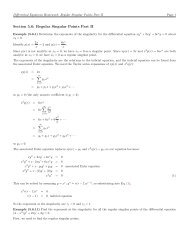
<strong>Section</strong> <strong>5.3</strong>: <strong>Series</strong> <strong>Solution</strong> <strong>Near</strong> <strong>Ordinary</strong> <strong>Point</strong>, <strong>Part</strong> <strong>II</strong><br />
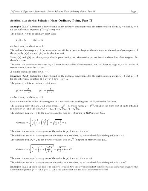
Example (<strong>5.3</strong>.5) Determine a lower bound on the radius of convergence for the series solution about x0 = 0 and x0 = 4<br />
for the differential equation y ′′ + 4y ′ + 6xy = 0.<br />
The point x0 = 0 is an ordinary point since<br />
p(x) = 4, q(x) = 6x<br />
are both analytic about x0 = 0.<br />
The radius of convergence of the series solution will be at least as large as the minimum of the radius of convergence of<br />
the series for p(x) = 4 and q(x) = 6x about x0 = 0.<br />
Since p(x) and q(x) are already expanded in power series, and these series are not infinite, the radius of convergence for<br />
them is ρ = ∞.<br />
Therefore, the series solution about x0 = 0 must have a radius of convergence that is at least as large as ρ = ∞, which of<br />
course means it must be ρ = ∞.<br />
A similar argument holds for x0 = 4.<br />
Example (<strong>5.3</strong>.7) Determine a lower bound on the radius of convergence for the series solution about x0 = 0 and x0 = 2<br />
for the differential equation (1 + x 3 )y ′′ + 4xy ′ + y = 0.<br />
The point x0 = 0 is an ordinary point since<br />
p(x) = 4x<br />
1<br />
, q(x) =<br />
1 + x3 1 + x3 are both analytic about x0 = 0.<br />
Let’s determine the radius of convergence of p and q without working out the Taylor series for them.<br />
The complex poles of p and q all occur when 1 − x 3 = 0, which means x = 1 1/3 , which is the third root of unity (studied<br />
in Chapter 4). These roots are x = −1, 1/2 + i √ 3/2, 1/2 − i √ 3/2.<br />
The distance from x0 = 0 to the nearest complex pole is 1 (diagram in Mathematica file).<br />
<br />
<br />
<br />
distance =<br />
1<br />
2<br />
2<br />
+<br />
√ 3<br />
2<br />
2<br />
=<br />
<br />
1 3<br />
+ = 1.<br />
4 4<br />
Therefore, the radius of convergence of the series for p(x) and q(x) is ρ = 1.<br />
The minimum radius of convergence for the series solution about x0 = 0 to the differential equation is ρ = 1.<br />
The distance from x0 = 2 to the nearest complex pole is √ 3 (diagram in Mathematica file).<br />
<br />
<br />
<br />
distance =<br />
<br />
2 − 1<br />
2<br />
2<br />
+<br />
√ 3<br />
2<br />
2<br />
=<br />
<br />
9 3<br />
+<br />
4 4 = √ 3.<br />
Therefore, the radius of convergence of the series for p(x) and q(x) is ρ = √ 3.<br />
The minimum radius of convergence for the series solution about x0 = 2 to the differential equation is ρ = √ 3.<br />
Example (<strong>5.3</strong>.11) Find the first four nonzero terms in two linearly independent series solutions about the origin to the<br />
differential equation y ′′ + (sin x)y = 0. What do you expect the radius of convergence to be?
Differential Equations Homework: <strong>Series</strong> <strong>Solution</strong> <strong>Near</strong> <strong>Ordinary</strong> <strong>Point</strong>, <strong>Part</strong> <strong>II</strong> Page 2<br />
First, since sin x has a series solution about x0 = 0 which converges for all x, we expect our series solution to converge for<br />
all x, which means the radius of convergence for the series solution should be ρ = ∞.<br />
We need to expand the sine function, if we hope to collect powers of x.<br />
sin x =<br />
∞<br />
(−1)<br />
n=0<br />
n x2n+1<br />
(2n + 1)! .<br />
Since p(x) = 0 and q(x) = sin x, which are analytic about x = 0, the point x = 0 is an ordinary point. Therefore, the<br />
assumed solution for the differential equation is<br />
y =<br />
y ′ =<br />
y ′′ =<br />
∞<br />
an(x − x0) n ∞<br />
= anx n<br />
n=0<br />
∞<br />
nanx n−1<br />
n=1<br />
∞<br />
n(n − 1)anx n−2<br />
n=2<br />
n=0<br />
Substitute into the differential equation:<br />
∞<br />
n=0<br />
∞<br />
n(n − 1)anx n−2 <br />
∞<br />
+<br />
n=2<br />
(n + 2)(n + 1)an+2x n +<br />
n=0<br />
∞<br />
n=0<br />
y ′′ + (sin x)y = 0<br />
<br />
∞<br />
anx<br />
(2n + 1)!<br />
n=0<br />
n<br />
<br />
= 0<br />
<br />
∞<br />
anx<br />
(2n + 1)!<br />
n<br />
<br />
= 0<br />
n x2n+1<br />
(−1)<br />
n x2n+1<br />
(−1)<br />
n=0<br />
Since we want to collect powers of x to get a recurrence relation, we have two options here. We can multiply out the two<br />
infinite series, or truncate all of them. There is an example of working with the infinite series multiplied together on a<br />
different differential equation at http://cda.mrs.umn.edu/ mcquarrb/DigitalDE/Math/SSOP.nb.<br />
Let’s truncate them here, and see what happens. Assuming that we will get both solutions at once, if we want the first<br />
four nonzero terms in each we should go out to at least x 8 . The manipulations that lead to the following equation are<br />
somewhat tedious, and I used Mathematica to perform them (they are in the associated Mathematica file).<br />
Let’s choose to truncate them all at k = 12 (I encourage to investigate this with the associated Mathematica file), and<br />
then we get the following:<br />
2a2 + (a0 + 6a3)x + (a1 + 12a4)x 2 <br />
+<br />
+<br />
+<br />
a0<br />
120<br />
− a2<br />
6 + a4 + 42a7<br />
<br />
x 5 +<br />
a1<br />
120<br />
<br />
− a1 a3 a5<br />
+ −<br />
5040 120 6 + a7 + 90a10<br />
− a0<br />
6 + a2 + 20a5<br />
− a3<br />
6 + a5 + 56a8<br />
<br />
x 8 + . . . = 0<br />
<br />
x 3 <br />
+<br />
<br />
x 6 +<br />
− a1<br />
6 + a3 + 30a6<br />
<br />
x 4<br />
<br />
− a0 a2 a4<br />
+ −<br />
5040 120 6 + a6 + 72a9<br />
Make sure you keep enough terms in the expansion so that you aren’t missing anything in the above. Set each coefficient<br />
of x to zero, and solve recursively for as many coefficients as you need (we were asked to get four nonzero terms in each<br />
solution).<br />
a0 = a0 unspecified, arbitrary not equal to zero<br />
a1 = a1 unspecified, arbitrary not equal to zero<br />
2a2 = 0 −→ a2 = 0<br />
<br />
x 7
Differential Equations Homework: <strong>Series</strong> <strong>Solution</strong> <strong>Near</strong> <strong>Ordinary</strong> <strong>Point</strong>, <strong>Part</strong> <strong>II</strong> Page 3<br />
a0 + 6a3 = 0 −→ a3 = − a0<br />
6<br />
a1 + 12a4 = 0 −→ a4 = − a1<br />
12<br />
− a0<br />
6 + a2 + 20a5 = 0 −→ a5 = a0<br />
120<br />
− a1<br />
6 + a3 + 30a6 = 0 −→ a6 = a1 a0<br />
+<br />
180 180<br />
a0 a2<br />
−<br />
120 6 + a4 + 42a7 = 0 −→ a7 = − a0 a1<br />
+<br />
5040 504<br />
We can actually stop here. Notice we only used the first six terms in our expansion.<br />
y(x) =<br />
∞<br />
anx n<br />
n=0<br />
= a0 + a1x + a2x 2 + a3x 3 + a4x 4 + a5x 5 + a6x 6 + a7x 7 + . . .<br />
= a0 + a1x − a0<br />
6 x3 − a1<br />
12 x4 + a0<br />
120 x5 + a1<br />
180 x6 + a0<br />
180 x6 − a0<br />
5040 x7 + a1<br />
504 x7 + . . .<br />
<br />
= a0 1 − x3<br />
<br />
x5 x6 x7<br />
+ + − + . . . + x −<br />
6 120 180 5040 x4<br />
<br />
x6 x7<br />
+ + + . . .<br />
12 180 504<br />
= a0y1(x) + a1y2(x)<br />
The two linearly independent solutions are<br />
y1(x) = 1 − x3<br />
6<br />
x5 x6 x7<br />
+ + − + . . .<br />
120 180 5040<br />
y2(x) = x − x4 x6 x7<br />
+ + + . . .<br />
12 180 504