MUS421/EE367B Lecture 2 Review of the Discrete Fourier Transform
MUS421/EE367B Lecture 2 Review of the Discrete Fourier Transform
MUS421/EE367B Lecture 2 Review of the Discrete Fourier Transform

You also want an ePaper? Increase the reach of your titles
YUMPU automatically turns print PDFs into web optimized ePapers that Google loves.
<strong>MUS421</strong>/<strong>EE367B</strong> <strong>Lecture</strong> 2<br />
<strong>Review</strong> <strong>of</strong> <strong>the</strong> <strong>Discrete</strong> <strong>Fourier</strong> <strong>Transform</strong> (DFT)<br />
Julius O. Smith III (jos@ccrma.stanford.edu)<br />
Center for Computer Research in Music and Acoustics (CCRMA)<br />
Department <strong>of</strong> Music, Stanford University<br />
Stanford, California 94305<br />
Outline<br />
• Domains <strong>of</strong> Definition<br />
February 21, 2012<br />
• <strong>Discrete</strong> <strong>Fourier</strong> <strong>Transform</strong><br />
• Properties <strong>of</strong> <strong>the</strong> <strong>Fourier</strong> <strong>Transform</strong><br />
For more details, see<br />
• Ma<strong>the</strong>matics <strong>of</strong> <strong>the</strong> DFT (Music 320 text):<br />
http://ccrma.stanford.edu/~jos/mdft/<br />
• Chapter 2 and Appendix B <strong>of</strong><br />
Spectral Audio Signal Processing (our text):<br />
http://ccrma.stanford.edu/~jos/sasp/<br />
1<br />
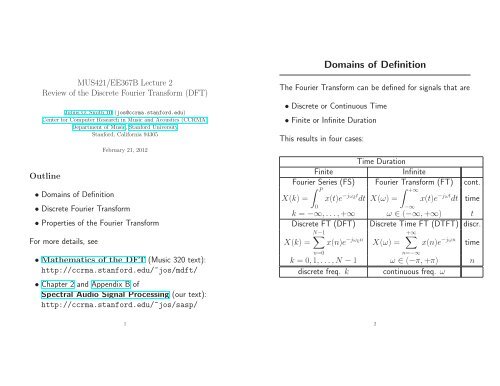
Domains <strong>of</strong> Definition<br />
The <strong>Fourier</strong> <strong>Transform</strong> can be defined for signals that are<br />
• <strong>Discrete</strong> or Continuous Time<br />
• Finite or Infinite Duration<br />
This results in four cases:<br />
Finite<br />
Time Duration<br />
Infinite<br />
<strong>Fourier</strong> Series (FS) <strong>Fourier</strong> <strong>Transform</strong> (FT) cont.<br />
X(k) =<br />
P<br />
0<br />
x(t)e −jω kt dt X(ω) =<br />
+∞<br />
−∞<br />
x(t)e −jωt dt time<br />
k = −∞,...,+∞ ω ∈ (−∞,+∞) t<br />
<strong>Discrete</strong> FT (DFT) <strong>Discrete</strong> Time FT (DTFT) discr.<br />
N−1 <br />
X(k) = x(n)e −jωkn +∞<br />
X(ω) = x(n)e −jωn<br />
time<br />
n=0<br />
n=−∞<br />
k = 0,1,...,N −1 ω ∈ (−π,+π) n<br />
discrete freq. k continuous freq. ω<br />
2
Geometric Interpretation <strong>of</strong> <strong>the</strong> <strong>Fourier</strong><br />
<strong>Transform</strong><br />
In all four cases,<br />
X(ω) = 〈x,sω〉<br />
where sω is a complex sinusoid at radian frequency ω<br />
rad/s:<br />
• e jωt (<strong>Fourier</strong> transform case),<br />
• e jωn (DTFT case),<br />
• e j2πkn/N (DFT case).<br />
Geometrically, X(ω) = 〈x,sω〉 is proportional to <strong>the</strong><br />
coefficient <strong>of</strong> projection <strong>of</strong> <strong>the</strong> signal x onto <strong>the</strong> signal sω.<br />
3<br />
Signal and <strong>Transform</strong> Notation<br />
• n,k ∈ Z (integers) or ZN (integers modulo N)<br />
• x(n) ∈ R (reals) or C (complex numbers)<br />
• x ∈ C N means x is a length N complex sequence<br />
• x = x(·)<br />
• X = DFT(x) ∈ C N , or<br />
x ↔ X<br />
where “↔” is read as “corresponds to”.<br />
• X(k) = DFTk(x) = DFTN,k(x) ∈ C<br />
• x(n) = IDFTn(X) = IDFTN,n(X)<br />
• For x ∈ C ∞ , X = DTFT(x) = DFT∞(x) ∈ C ∞ 2π<br />
• x = conjugate <strong>of</strong> x<br />
• ∠x = phase <strong>of</strong> x<br />
The notation XY or X ·Y denotes <strong>the</strong> vector containing<br />
(XY)k = X(k)Y(k), k = 0,...,N −1. This is denoted<br />
by ‘X .* Y’ in Matlab, where X and Y may a pair <strong>of</strong><br />
column vectors, or a pair <strong>of</strong> row vectors.<br />
4
The <strong>Discrete</strong> <strong>Fourier</strong> <strong>Transform</strong><br />
The “kth bin” <strong>of</strong> <strong>the</strong> <strong>Discrete</strong> <strong>Fourier</strong> <strong>Transform</strong> (DFT)<br />
is defined as<br />
X(k) ∆ = DFTk(x) ∆ = 〈x,sk〉 ∆ =<br />
N−1 <br />
n=0<br />
sk(n) ∆ = e jω ktn ; k = 0,1,...,N −1<br />
ωk<br />
∆<br />
= 2π k<br />
N fs = 2πk<br />
NT<br />
; tn<br />
∆<br />
= nT<br />
x(tn)e −jω ktn<br />
We may interpret <strong>the</strong> DFT as <strong>the</strong> coefficients <strong>of</strong><br />
projection <strong>of</strong> <strong>the</strong> signal vector x onto <strong>the</strong> N sinusoidal<br />
basis signals sk, k = 0,1,...,N −1:<br />
X(k) = 〈x,sk〉<br />
5<br />
The inverse DFT is given by<br />
x(tn) =<br />
N−1 <br />
k=0<br />
Inverse DFT<br />
〈x,sk〉<br />
sk 2sk(tn) = 1<br />
N−1 <br />
N<br />
k=0<br />
X(ωk)e jω ktn<br />
It can be interpreted as <strong>the</strong> superposition <strong>of</strong> <strong>the</strong><br />
projections, i.e., <strong>the</strong> sum <strong>of</strong> <strong>the</strong> sinusoidal basis signals<br />
weighted by <strong>the</strong>ir respective coefficients <strong>of</strong> projection:<br />
x = <br />
k<br />
〈x,sk〉<br />
sk 2sk<br />
6
The DFT, Cont’d<br />
There are several ways to think about <strong>the</strong> DFT:<br />
1. Projection onto <strong>the</strong> set <strong>of</strong> “basis” sinusoids<br />
(frequencies at N roots <strong>of</strong> unity)<br />
2. Coordinate transformation (“natural” R N basis to<br />
“sinusoidal” basis)<br />
3. Matrix multiplication X = W ∗ x,<br />
where W ∗ [k,n] = e −jω ktn<br />
4. Sampled uniform filter bank output<br />
This course will emphasize interpretations 1 and 4.<br />
7<br />
Properties <strong>of</strong> <strong>the</strong> DFT<br />
We are going to be performing manipulations on signals<br />
and <strong>the</strong>ir <strong>Fourier</strong> <strong>Transform</strong> throughout this class. It is<br />
important to understand how changes we make in one<br />
domain affect <strong>the</strong> o<strong>the</strong>r domain. The <strong>Fourier</strong> <strong>the</strong>orems<br />
are helpful for this purpose.<br />
Derivations <strong>of</strong> <strong>the</strong> <strong>Fourier</strong> <strong>the</strong>orems for <strong>the</strong> DTFT case<br />
may be found in Chapter 2 <strong>of</strong> <strong>the</strong> text, and in<br />
Ma<strong>the</strong>matics <strong>of</strong> <strong>the</strong> DFT 1 (Music 320 text) for <strong>the</strong><br />
DFT case.<br />
1 http://ccrma.stanford.edu/~jos/mdft/<strong>Fourier</strong> Theorems.html<br />
8
or<br />
Linearity<br />
αx1+βx2 ↔ αX1+βX2<br />
DFT(αx1+βx2) = α·DFT(x1)+β ·DFT(x2)<br />
α,β ∈ C<br />
x1,x2,X1,X2 ∈ C N<br />
The <strong>Fourier</strong> <strong>Transform</strong> “commutes with mixing.”<br />
9<br />
Symmetries for Real Signals<br />
If a time-domain signal x is real, <strong>the</strong>n its <strong>Fourier</strong><br />
transform X is conjugate symmetric (Hermitian):<br />
or<br />
Hermitian symmetry implies<br />
x ∈ R N ⇔ X(−k) = X(k)<br />
Real ↔ Hermitian<br />
• Real part Symmetric (even):<br />
re{X(−k)} = re{X(k)}<br />
• Imaginary part Antisymmetric (skew-symmetric, odd):<br />
im{X(−k)} = −im{X(k)}<br />
• Magnitude Symmetric (even):<br />
|X(−k)| = |X(k)|<br />
• Phase Antisymmetric (odd):<br />
∠X(−k) = −∠X(k)<br />
10
Definition:<br />
Time Reversal<br />
Flipn(x) ∆ = x(−n) ∆ = x(N −n)<br />
Note: x(n) ∆ = x(nmodN) for signals in C N (DFT<br />
case).<br />
When computing a sampled DTFT using <strong>the</strong> DFT, we<br />
interpret time indices n = 1,2,...,N/2−1 as positive<br />
time indices, and n = N −1,N −2,...,N/2 as <strong>the</strong><br />
negative time indices n = −1,−2,...,−N/2. Under<br />
this interpretation, <strong>the</strong> Flip operator simply reverses a<br />
signal in time.<br />
<strong>Fourier</strong> <strong>the</strong>orems:<br />
Flip(x) ↔ Flip(X)<br />
for x ∈ C N . In <strong>the</strong> typical special case <strong>of</strong> real signals<br />
(x ∈ R N ), we have Flip(X) = X so that<br />
Flip(x) ↔ X<br />
Time-reversing a real signal conjugates its spectrum<br />
Shift Theorem<br />
11<br />
The Shift operator is defined as Shiftl,n(y) ∆ = y(n−l).<br />
Since indexing is defined modulo N, Shiftl(y) is a<br />
circular right-shift by l samples.<br />
or, more loosely,<br />
i.e.,<br />
Shiftl(y) ↔ e −j(·)l Y<br />
y(n−l) ↔ e −jωl Y(ω)<br />
DFTk[Shiftl(y)] = e −jω kl Y(ωk)<br />
e −jω kl = Linear Phase Term, slope = −l<br />
• ∠Y(ωk)+= −ωkl<br />
• Multiplying a spectrum Y by a linear phase term<br />
e −jω kl with phase slope −l corresponds to a circular<br />
right-shift in <strong>the</strong> time domain by l samples:<br />
• negative slope ⇒ time delay<br />
• positive slope ⇒ time advance<br />
12
Convolution<br />
The cyclic convolution <strong>of</strong> x and y is defined as<br />
(x∗y)(n) ∆ =<br />
N−1 <br />
m=0<br />
x(m)y(n−m), x,y ∈ C N<br />
Cyclic convolution is also called circular convolution,<br />
since y(n−m) ∆ = y(n−m(mod N)).<br />
Convolution is cyclic in <strong>the</strong> time domain for <strong>the</strong> DFT and<br />
FS cases, and acyclic for <strong>the</strong> DTFT and FT cases.<br />
The Convolution Theorem is <strong>the</strong>n<br />
(x∗y) ↔ X ·Y<br />
13<br />
Linear Convolution <strong>of</strong> Short Signals<br />
x(t) h y(t) = (x∗h)(t)<br />
Convolution <strong>the</strong>orem for DFTs:<br />
or<br />
(h∗x) ↔ H ·X<br />
DFTk(h∗x) = H(ωk)X(ωk)<br />
where h,x ∈ C N , and H and X are <strong>the</strong> N-point DFTs<br />
<strong>of</strong> h and x, respectively.<br />
DFT performs circular (or cyclic) convolution:<br />
y(n) ∆ = (x∗h)(n) ∆ =<br />
N−1 <br />
m=0<br />
x(m)h(n−m)N<br />
where (n−m)N means “(n−m) modulo N”<br />
Ano<strong>the</strong>r way to look at this is as <strong>the</strong> inner product <strong>of</strong> x,<br />
and Shiftn[Flip(h)], i.e.,<br />
y(n) = 〈x,Shiftn[Flip(h)]〉<br />
14
FFT Convolution<br />
The convolution <strong>the</strong>orem h∗x ↔ H ·X shows us that<br />
<strong>the</strong>re are two ways to perform circular convolution.<br />
• direct calculation <strong>of</strong> <strong>the</strong> summation = O(N 2 )<br />
• frequency-domain approach = O(NlgN)<br />
• <strong>Fourier</strong> <strong>Transform</strong> both signals<br />
• Perform term by term multiplication <strong>of</strong> <strong>the</strong><br />
transformed signals<br />
• Inverse transform <strong>the</strong> result to get back to <strong>the</strong><br />
time domain<br />
Remember ... this still gives us cyclic convolution<br />
Idea: If we add enough trailing zeros to <strong>the</strong> signals<br />
being convolved, we can get <strong>the</strong> same results as in acyclic<br />
convolution (in which <strong>the</strong> convolution summation goes<br />
from m = 0 to ∞).<br />
Question: How many zeros do we need to add?<br />
N x<br />
N N N<br />
∗ =<br />
N h<br />
15<br />
N x +N h -1<br />
• If we perform an acyclic convolution <strong>of</strong> two signals, x<br />
and h, with lengths Nx and Nh, <strong>the</strong> resulting signal is<br />
length Ny = Nx+Nh−1.<br />
• Therefore, to implement acyclic convolution using <strong>the</strong><br />
DFT, we must add enough zeros to x and y so that<br />
<strong>the</strong> cyclic convolution result is length Ny or longer.<br />
• If we don’t add enough zeros, some <strong>of</strong> our<br />
convolution terms “wrap around” and add back<br />
upon o<strong>the</strong>rs (due to modulo indexing).<br />
• This can be called time domain aliasing.<br />
• We typically zero-pad even fur<strong>the</strong>r (to <strong>the</strong> next power<br />
<strong>of</strong> 2) so we can use <strong>the</strong> Cooley-Tukey FFT for<br />
maximum speed<br />
A sampling-<strong>the</strong>orem based insight:<br />
Zero-padding in <strong>the</strong> time domain results in more samples<br />
(closer spacing) in <strong>the</strong> frequency domain. This can be<br />
thought <strong>of</strong> as a higher ‘sampling rate’ in <strong>the</strong> frequency<br />
domain. If we have a high enough frequency-domain<br />
sampling rate, we can avoid time domain aliasing.<br />
16
Example FFT Convolution<br />
% matlab/fftconvexample.m<br />
x = [1 2 3 4 5 6];<br />
h = [1 1 1];<br />
nx = length(x);<br />
nh = length(h);<br />
nfft = 2^nextpow2(nx+nh-1)<br />
xzp = [x, zeros(1,nfft-nx)];<br />
hzp = [h, zeros(1,nfft-nh)];<br />
X = fft(xzp);<br />
H = fft(hzp);<br />
Y = H .* X;<br />
y = real(ifft(Y))<br />
Program output:<br />
octave:10> fftconvexample<br />
nfft = 8<br />
y =<br />
1 3 6 9 12 15 11 6<br />
17<br />
FFT Convolution vs. Direct Convolution<br />
Let’s compare <strong>the</strong> number <strong>of</strong> operations needed to<br />
perform <strong>the</strong> convolution <strong>of</strong><br />
2 length N sequences:<br />
• It takes ≈ N 2 multiply/add operations to calculate<br />
<strong>the</strong> convolution summation directly.<br />
• It takes on <strong>the</strong> order <strong>of</strong> N ·log(N) operations to<br />
compute an FFT. (Note: H(ωk) can be calculated in<br />
advance for time-invariant filtering.)<br />
N FFT Direct Convolution<br />
4 176 16<br />
32 2560 1024<br />
64 5888 4096<br />
128 13,312 16,384<br />
256 29,696 65,536<br />
2048 311,296 4,194,304<br />
In this example (from Strum and Kirk), <strong>the</strong> FFT<br />
(s<strong>of</strong>tware) beats direct time-domain convolution at length<br />
128 and higher<br />
18
Correlation<br />
The cross-correlation <strong>of</strong> x and y in C N is defined as:<br />
(x⋆y)(n) ∆ =<br />
N−1 <br />
m=0<br />
x(m)y(n+m), x,y ∈ C N<br />
Using this definition we have <strong>the</strong> correlation <strong>the</strong>orem:<br />
(x⋆y) ↔ X(ωk)Y(ωk)<br />
The correlation <strong>the</strong>orem is <strong>of</strong>ten used in <strong>the</strong> context <strong>of</strong><br />
spectral analysis <strong>of</strong> filtered noise signals.<br />
Autocorrelation<br />
The autocorrelation <strong>of</strong> a signal x ∈ C N is simply <strong>the</strong><br />
cross-correlation <strong>of</strong> x with itself:<br />
(x⋆x)(n) ∆ =<br />
N−1 <br />
m=0<br />
x(m)x(m+n), x ∈ C N<br />
From <strong>the</strong> correlation <strong>the</strong>orem, we have<br />
(x⋆x) ↔ |X(ωk)| 2<br />
19<br />
Power Theorem<br />
The inner product <strong>of</strong> two signals is defined as:<br />
〈x,y〉 ∆ = <br />
n<br />
xny n<br />
Using this notation, we have <strong>the</strong> following:<br />
〈x,y〉 = 1<br />
N 〈X,Y〉<br />
When we consider <strong>the</strong> inner product <strong>of</strong> a signal with itself,<br />
we have a special case known as Parseval’s Theorem:<br />
x 2 = 〈x,x〉 = 1 X2<br />
〈X,X〉 =<br />
N N<br />
(Also called <strong>the</strong> Rayleigh’s Energy Theorem.)<br />
20
Stretch<br />
We define <strong>the</strong> Stretch operator such that:<br />
StretchL : C N → C NL<br />
Which means that it transforms a length N complex<br />
signal, into a length NL signal. Specifically, we do this<br />
by inserting L−1 zeros in between each pair <strong>of</strong> samples<br />
<strong>of</strong> <strong>the</strong> signal.<br />
x<br />
y = Stretch 2 (x) →<br />
...<br />
21<br />
y<br />
...<br />
Repeat or Scale<br />
Similarly, <strong>the</strong> RepeatL operator, defined on <strong>the</strong> unit<br />
circle, frequency-scales its input spectrum by <strong>the</strong> factor L:<br />
ω ← Lω<br />
The original spectrum is repeated L times as ω traverses<br />
<strong>the</strong> unit circle. This is illustrated in <strong>the</strong> following diagram<br />
for L = 2:<br />
X<br />
Y = REPEAT 3 (X) →<br />
ω<br />
Using <strong>the</strong>se definitions, we have <strong>the</strong> Stretch Theorem:<br />
StretchL(x) ↔ RepeatL(X)<br />
Application: Upsampling by any integer factor L:<br />
Passing <strong>the</strong> stretched signal through an ideal lowpass<br />
filter cutting <strong>of</strong>f at ω ≥ π/L yields ideal bandlimited<br />
interpolation <strong>of</strong> <strong>the</strong> original signal by <strong>the</strong> factor L.<br />
22<br />
Y<br />
ω
Zero-Padding ↔ Interpolation<br />
Zero padding in <strong>the</strong> time domain corresponds to ideal<br />
interpolation in <strong>the</strong> frequency domain.<br />
Pro<strong>of</strong>:<br />
http://ccrma.stanford.edu/~jos/mdft/Zero Padding Theorem Spectral.html<br />
Downsampling ↔ Aliasing<br />
The downsampling operation DownsampleM selects<br />
every M th sample <strong>of</strong> a signal:<br />
DownsampleM,n(x) ∆ = x(Mn)<br />
In <strong>the</strong> DFT case, DownsampleM maps C N to C N M,<br />
while for <strong>the</strong> DTFT, DownsampleM maps C ∞ to C ∞ .<br />
The Aliasing Theorem states that downsampling in time<br />
corresponds to aliasing in <strong>the</strong> frequency domain:<br />
DownsampleM(x) ↔ 1<br />
M AliasM(X)<br />
where <strong>the</strong> Alias operator is defined for X ∈ C N<br />
23<br />
(DFT case) as<br />
AliasM,l(X) ∆ =<br />
M−1 <br />
k=0<br />
X<br />
<br />
l+k N<br />
<br />
, l = 0,1,...,<br />
M<br />
N<br />
M −1<br />
For X ∈ C ∞ (DTFT case), <strong>the</strong> Alias operator is<br />
AliasM,ω(X) ∆ =<br />
∆<br />
=<br />
M−1 <br />
k=0<br />
M−1<br />
X<br />
<br />
X<br />
k=0<br />
<br />
e j( ω M +k2π<br />
M )<br />
<br />
, −π ≤ ω < π<br />
<br />
W k Mz 1 <br />
M<br />
∆<br />
where WM = ej2π/M is a common notation for <strong>the</strong><br />
primitive Mth root <strong>of</strong> unity, and z = ejω as usual. This<br />
normalization corresponds to T = 1 after downsampling.<br />
Thus, T = 1/M prior to downsampling.<br />
The summation terms above for k = 0 are called aliasing<br />
components.<br />
The aliasing <strong>the</strong>orem points out that in order to<br />
downsample by factor M without aliasing, we must first<br />
lowpass-filter <strong>the</strong> spectrum to [−πfs/M,πfs/M]. This<br />
filtering essentially zeroes out <strong>the</strong> spectral regions which<br />
alias upon sampling.<br />
24
Recall:<br />
where<br />
Ideal Spectral Interpolation<br />
sω(t) ∆ = e jωt<br />
X(ω) ∆ = 〈x,sω〉<br />
sω(tn) ∆ = e jωtn ∆ = e jωn<br />
(FT)<br />
(DTFT)<br />
For signals in <strong>the</strong> DTFT domain which happen to be time<br />
limited to n ∈ [−N/2,N/2−1],<br />
X(ω) ∆ = 〈x,sω〉 =<br />
∞<br />
n=−∞<br />
x(n)e −jωn =<br />
N/2−1 <br />
n=−N/2<br />
• This can be interpreted as a 0-centered DFT<br />
evaluated at ω instead <strong>of</strong> ωk = 2πk/N.<br />
• It arises as <strong>the</strong> DTFT <strong>of</strong> a finite-length signal.<br />
• Time-limited signals may be said to have “finite<br />
support.”<br />
x(n)e −jωn<br />
• Such signals can be sampled at ω = ωk = 2πk/N<br />
without loss <strong>of</strong> information<br />
25<br />
Meaning <strong>of</strong> Spectral Interpolation<br />
• Let X(ωk) denote <strong>the</strong> spectrum to be interpolated.<br />
• Then <strong>the</strong> corresponding time signal is<br />
x = IDFTN(X).<br />
• We define <strong>the</strong> spectral interpolation X(ω) as <strong>the</strong><br />
projection <strong>of</strong> our signal x onto an arbitrary sinusoid<br />
sω = e jωnT .<br />
• This is equivalent to X(ω) = DTFTω(x):<br />
X(ω) ∆ = 〈x,sω〉 = <br />
n<br />
x(n)e −jωnT<br />
= DTFTω{···0,x,0,...}<br />
≈ FFTω k {ZeroPadL{x}}<br />
for some sufficiently large zero-padding factor L.<br />
• In <strong>the</strong> Quadratically Interpolated FFT (QIFFT)<br />
method for measuring parameters <strong>of</strong> spectral peaks,<br />
we will choose L to be sufficient in conjunction with<br />
quadratic interpolation <strong>of</strong> spectral log magnitude<br />
samples at each peak<br />
26
Interpolating a DFT<br />
Starting with a sampled spectrum X(ωk),<br />
k = 0,1,...,N −1, we may interpolate ideally by taking<br />
<strong>the</strong> DTFT <strong>of</strong> <strong>the</strong> zero-padded IDFT:<br />
X(ω) = DTFTω(ZeroPad∞(IDFTN(X)))<br />
N/2−1 N−1<br />
∆ 1 <br />
= X(ωk)e<br />
N<br />
n=−N/2 k=0<br />
jω <br />
kn<br />
e −jωn<br />
⎡<br />
N−1 <br />
= X(ωk) ⎣ 1<br />
N/2−1 <br />
e<br />
N<br />
j(ω ⎤<br />
k−ω)n⎦<br />
=<br />
k=0<br />
N−1 <br />
n=−N/2<br />
X(ωk)asincN(ω −ωk)<br />
k=0<br />
= X,SampleΩ (Shiftω(asincN)) N <br />
= (X ⊛asincN)ω,<br />
where ⊛ denotes convolution between a discrete (X) and<br />
continuous (asinc) signal. (If math operators adapt to<br />
<strong>the</strong>ir argument types like perl functions, we can simply<br />
use ∗ as usual.)<br />
• Zero-padding in <strong>the</strong> time domain corresponds to<br />
“asincN interpolation” in <strong>the</strong> frequency domain<br />
• This is “ideal time-limited spectral interpolation”<br />
27<br />
Practical Zero Padding<br />
To interpolate a uniformly sampled spectrum X(ωk) by<br />
<strong>the</strong> factor L, we may take <strong>the</strong> inverse DFT, append<br />
zeros, and take <strong>the</strong> FFT (which is very fast):<br />
X(ωl) = FFTLN,l(ZeroPadLN(IDFTN(X))),<br />
l = 0,...,LN −1<br />
This operation creates L−1 new bins between each pair<br />
<strong>of</strong> original bins in X, thus increasing <strong>the</strong> number <strong>of</strong><br />
spectral samples around <strong>the</strong> unit circle from N to LN.<br />
In matlab, we can specify zero-padding by simply<br />
providing <strong>the</strong> optional FFT-size argument:<br />
X = fft(x,N); % FFT size N > length(x)<br />
28
Reasons for Zero Padding<br />
(Spectral Interpolation)<br />
• Zero-padding makes our FFTs look like DTFTs when<br />
displaying spectra.<br />
• Zero-padding enables us to use <strong>the</strong> FFT with any<br />
window length M. When M is not a power <strong>of</strong> 2, we<br />
append enough zeros to make <strong>the</strong> FFT size N > M a<br />
power <strong>of</strong> 2.<br />
• For sinusoidal peak-finding, spectral interpolation via<br />
zero-padding gets us closer to <strong>the</strong> true maximum <strong>of</strong><br />
<strong>the</strong> main lobe when we simply take <strong>the</strong><br />
maximum-magnitude FFT-bin as our estimate.<br />
29<br />
Zero Padding Examples<br />
Let’s look at <strong>the</strong> effect <strong>of</strong> zero padding on <strong>the</strong> <strong>Fourier</strong><br />
transform <strong>of</strong> <strong>the</strong> popular (causal) Hamming window:<br />
<br />
2πn<br />
w(n) = 0.54−0.46 cos , n = 0,1,2,...M −1<br />
M<br />
where M = 21 in our examples.<br />
We will look at shifts <strong>of</strong> <strong>the</strong><br />
• critically sampled window transform W(ωk−ω0), and<br />
• 2× oversampled window transform W(ω k ′ −ω0)<br />
where ω0 = 2π ·3/M = 2π/7 ≈ 0.9 rad/samp is <strong>the</strong><br />
normalized radian frequency <strong>of</strong> <strong>the</strong> test sinusoid to which<br />
<strong>the</strong> window is applied.<br />
30
Critically Sampled Hamming Window <strong>Transform</strong><br />
Consider performing a length M DFT on a length M<br />
windowed signal:<br />
• N ∆ = DFT size = M ∆ = Window length<br />
• DFT frequency samples at ωk = k 2π<br />
M<br />
(critically sampled DTFT)<br />
• Window sequence and windowed-sinusoid spectrum:<br />
(a)<br />
(b)<br />
Amplitude<br />
Magnitude (dB)<br />
1<br />
0.8<br />
0.6<br />
0.4<br />
0.2<br />
Causal Hamming window − M = 21 − no zero padding<br />
0<br />
0 2 4 6 8 10<br />
Time (samples)<br />
12 14 16 18 20<br />
−10<br />
−20<br />
−30<br />
−40<br />
−50<br />
−60<br />
0 0.5 1 1.5 2 2.5 3<br />
Normalized Frequency (radians/sample)<br />
• DFT bin width = 2π<br />
N<br />
= 2π<br />
M<br />
(critically sampled)<br />
• 4 samples per main lobe (Hamming window)<br />
31<br />
2X Oversampled Hamming Window <strong>Transform</strong><br />
Let’s now zero-pad by a factor <strong>of</strong> 2 in <strong>the</strong> time domain,<br />
before we perform our DFT:<br />
• Zero-padding factor L ∆ = N<br />
M<br />
• N = DFT size = 2M<br />
= 2<br />
• DFT frequency samples at ω k ′ = k ′2π<br />
N<br />
= k′ 2π<br />
2M<br />
Causal zero-padding by a factor <strong>of</strong> two (L = 2):<br />
(a)<br />
(b)<br />
Amplitude<br />
Magnitude (dB)<br />
1<br />
0.8<br />
0.6<br />
0.4<br />
0.2<br />
Causal Hamming window − M = 21 − zero padding factor = 2<br />
0<br />
0 5 10 15 20 25 30 35 40 45<br />
Time (samples)<br />
−10<br />
−20<br />
−30<br />
−40<br />
−50<br />
−60<br />
0 0.5 1 1.5 2 2.5 3<br />
Normalized Frequency (radians/sample)<br />
• DFT bin width = 1<br />
2π<br />
LM<br />
= 2π<br />
2M<br />
(2× oversampled)<br />
• 8 samples per main lobe (Hamming window)<br />
32
Oversampled Spectral Peaks<br />
Note that zero-padding helps in finding <strong>the</strong> true peak <strong>of</strong><br />
<strong>the</strong> sampled window transform.<br />
Magnitude (linear)<br />
1<br />
0.8<br />
0.6<br />
0.4<br />
0.2<br />
zero pad factor = 8<br />
0<br />
0 0.5 1 1.5 2 2.5 3<br />
Normalized Frequency (radians/sample)<br />
33<br />
(a)<br />
(b)<br />
Zero-Centered Zero-Padding<br />
Amplitude<br />
Amplitude<br />
1<br />
0.5<br />
0<br />
−0.5<br />
Blackman Windowed Sinusoid<br />
−1<br />
−15 −10 −5 0<br />
Time (samples)<br />
5 10 15<br />
1<br />
0.5<br />
0<br />
−0.5<br />
positive time negative time<br />
−1<br />
0 10 20 30<br />
Time (samples)<br />
40 50 60<br />
(a) Blackman window overlaid with windowed data.<br />
(b) Zero-padded and loaded into FFT input buffer.<br />
• Use zero-centered zero padding with zero-phase<br />
windows<br />
• Use causal zero padding with causal windows<br />
34
(a)<br />
(b)<br />
Magnitude (linear)<br />
Magnitude (linear)<br />
8<br />
6<br />
4<br />
2<br />
Zero-Centered Spectra<br />
positive frequencies negative frequencies<br />
0<br />
0 10 20 30<br />
Frequency (bins))<br />
40 50 60<br />
8<br />
6<br />
4<br />
2<br />
negative frequencies positive frequencies<br />
0<br />
−30 −20 −10 0<br />
Frequency (bins))<br />
10 20 30<br />
(a) FFT magnitude data, as returned by <strong>the</strong> FFT.<br />
(b) FFT magnitude spectrum “rotated” to a more<br />
“physical” frequency axis in bin numbers.<br />
35<br />
fftshift<br />
Matlab and Octave have a simple utility called fftshift<br />
that performs this bin rotation. Consider <strong>the</strong> following<br />
example:<br />
octave:4><br />
fftshift([1 2 3 4])<br />
ans =<br />
3 4 1 2<br />
octave:5><br />
Note that both Matlab and Octave regard <strong>the</strong> spectral<br />
sample at half <strong>the</strong> sampling rate as a negative frequency.<br />
For odd N, <strong>the</strong> only reasonable answer is<br />
octave:4><br />
fftshift([1 2 3])<br />
ans =<br />
3 1 2<br />
octave:5><br />
corresponding to frequencies −fs/3,0,fs/3, respectively.<br />
36