Articles - CCRMA - Stanford University

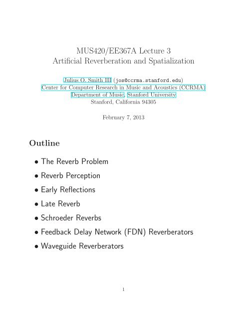
MUS420/EE367A Lecture 3
Artificial Reverberation and Spatialization
Julius O. Smith III (jos@ccrma.stanford.edu)
Center for Computer Research in Music and Acoustics (CCRMA)
Department of Music, Stanford University
Stanford, California 94305
Outline
• The Reverb Problem
• Reverb Perception
• Early Reflections
• Late Reverb
• Schroeder Reverbs
February 7, 2013
• Feedback Delay Network (FDN) Reverberators
• Waveguide Reverberators
1

s1(n)
s2(n)
s3(n)
Reverberation Transfer Function
• Three sources
h11
h12
h13
h21
h22
h23
• One listener (two ears)
• Filters should include pinnae filtering
(spatialized reflections)
• Filters change if anything in the room changes
In principle, this is an exact computational model.
2
y1(n)
y2(n)

Implementation
Let hij(n) = impulse response from source j to ear i.
Then the output is given by six convolutions:
y1(n) = (s1∗h11)(n)+(s2∗h12)(n)+(s3∗h13)(n)
y2(n) = (s1∗h21)(n)+(s2∗h22)(n)+(s3∗h23)(n)
• For small n, filters hij(n) are sparse
• Tapped Delay Line (TDL) a natural choice
Transfer-function matrix:
Y1(z) H11(z) H12(z) H13(z)
=
Y2(z) H21(z) H22(z) H23(z)
⎡
⎣
3
S1(z)
S2(z)
S3(z)
⎤
⎦

Complexity of Exact Reverberation
Reverberation time is typically defined as t60, the time, in
seconds, to decay by 60 dB.
Example:
• Let t60 = 1 second
• fs = 50 kHz
• Each filter hij requires 50,000 multiplies and additions
per sample, or 2.5 billion multiply-adds per second.
• Three sources and two listening points (ears) ⇒
30 billion operations per second
– 10 dedicated CPUs clocked at 3 Gigahertz
– multiply and addition initiated each clock cycle
– no wait-states for parallel input, output, and filter
coefficient accesses
• FFT convolution is faster, if throughput delay is
tolerable (and there are low-latency algorithms)
Conclusion: Exact implementation of point-to-point
transfer functions is generally too expensive for real-time
computation.
4

Possibility of a Physical Reverb Model
In a complete physical model of a room,
• sources and listeners can be moved without affecting
the room simulation itself,
• spatialized (in 3D) stereo output signals can be
extracted using a “virtual dummy head”
How expensive is a room physical model?
• Audio bandwidth = 20 kHz ≈ 1/2 inch wavelength
• Spatial samples every 1/4 inch or less
• A 12’x12’x8’ room requires > 100 million grid points
• A lossless 3D finite difference model requires one
multiply and 6 additions per grid point ⇒ 30 billion
additions per second at fs = 50 kHz
• A 100’x50’x20’ concert hall requires more than
3 quadrillion operations per second
Conclusion: Fine-grained physical models are too
expensive for real-time computation, especially for large
halls.
5

Perceptual Aspects of Reverberation
Artificial reverberation is an unusually interesting signal
processing problem:
• “Obvious” methods based on physical modeling or
input-output modeling are too expensive
• We do not perceive the full complexity of
reverberation
• What is important perceptually?
• How can we simulate only what is audible?
6

Perception of Echo Density and Mode Density
• For typical rooms
– Echo density increases as t 2
– Mode density increases as f 2
• Beyond some time, the echo density is so great that a
stochastic process results
• Above some frequency, the mode density is so great
that a random frequency response results
• There is no need to simulate many echoes per sample
• There is no need to implement more resonances than
the ear can hear
7

Proof that Echo Density Grows as Time Squared
Consider a single spherical wave produced from a point
source in a rectangular room.
• Tesselate 3D space with copies of the original room
• Count rooms intersected by spherical wavefront
8

Proof that Mode Density Grows as Freq. Squared
The resonant modes of a rectangular room are given by 1
k 2 (l,m,n) = k 2 x(l)+k 2 y(m)+k 2 z(n)
• kx(l) = lπ/Lx = lth harmonic of the fundamental
standing wave in the x
• Lx = length of the room along x
• Similarly for y and z
• Mode frequencies map to a uniform 3D Cartesian grid
indexed by (l,m,n)
• Grid spacings are π/Lx, π/Ly, and π/Lz in x,y, and
z, respectively.
• Spatial frequency k of mode (l,m,n) = distance
from the (0,0,0) to (l,m,n)
• Therefore, the number of room modes having a given
spatial frequency grows as k 2
1 For a tutorial on vector wavenumber, see Appendix E, section E.6.5, in the text:
http://ccrma.stanford.edu/˜jos/pasp/Vector Wavenumber.html
9

Early Reflections and Late Reverb
Based on limits of perception, the impulse response of a
reverberant room can be divided into two segments
• Early reflections = relatively sparse first echoes
• Late reverberation—so densely populated with echoes
that it is best to characterize the response
statistically.
Similarly, the frequency response of a reverberant room
can be divided into two segments.
• Low-frequency sparse distribution of resonant modes
• Modes packed so densely that they merge to form a
random frequency response with regular statistical
properties
10

Perceptual Metrics for Ideal Reverberation
Some desirable controls for an artificial reverberator
include
• t60(f) = desired reverberation time at each frequency
• G 2 (f) = signal power gain at each frequency
• C(f) = “clarity” = ratio of impulse-response energy
in early reflections to that in the late reverb
• ρ(f) = inter-aural correlation coefficient at left and
right ears
Perceptual studies indicate that reverberation time t60(f)
should be independently adjustable in at least three
frequency bands.
11

Energy Decay Curve (EDC)
For measuring and defining reverberation time t60,
Schroeder introduced the so-called energy decay curve
(EDC) which is the tail integral of the squared impulse
response at time t:
EDC(t) ∆ =
∞
t
h 2 (τ)dτ
• EDC(t) = total signal energy remaining in the
reverberator impulse response at time t
• EDC decays more smoothly than the impulse response
itself
• Better than ordinary amplitude envelopes for
estimating t60
12

Energy Decay Relief (EDR)
The energy decay relief (EDR) generalizes the EDC to
multiple frequency bands:
EDR(tn,fk) ∆ M
= |H(m,k)| 2
m=n
where H(m,k) denotes bin k of the short-time Fourier
transform (STFT) at time-frame m, and M is the
number of frames.
• FFT window length ≈ 30−40 ms
• EDR(tn,fk) = total signal energy remaining at time
tn sec in frequency band centered at fk
13

Magnitude (dB)
Energy Decay Relief (EDR) of a Violin Body
Impulse Response
40
20
0
−20
−40
−60
bodyv6t − Summed EDR
−80
0 2 4 6 8 10 12 14 16 18
Band Centers (kHz)
5
4
3
2
1
Time (frames)
• Energy summed over frequency within each “critical
band of hearing” (Bark band)
• Violin body = “small box reverberator”
14

x(n)
Reverb = Early Reflections + Late Reverb
Tapped Delay Line
... ...
Late
Reverb
• TDL taps may include lowpass filters
(air absorption, lossy reflections)
• Several taps may be fed to late reverb unit,
especially if it takes a while to reach full density
• Some or all early reflections can usually be worked
into the delay lines of the late-reverberation
simulation (transposed tapped delay line)
15
y(n)

Early Reflections
The “early reflections” portion of the impulse response is
defined as everything up to the point at which a statistical
description of the late reverb becomes appropriate
• Often taken to be the first 100ms
• Better to test for Gaussianness
– Histogram test for sample amplitudes in 10ms
windows
– Exponential fit (t60 match) to EDC (Prony’s
method, matrix pencil method)
– Crest factor test (peak/rms)
• Typically implemented using tapped delay lines (TDL)
(suggested by Schroeder in 1970 and implemented by
Moorer in 1979)
• Early reflections should be spatialized (Kendall)
• Early reflections influence spatial impression
16

Desired Qualities:
Late Reverberation
1. a smooth (but not too smooth) decay, and
2. a smooth (but not too regular) frequency response.
• Exponential decay no problem
• Hard part is making it smooth
– Must not have “flutter,” “beating,” or unnatural
irregularities
– Smooth decay generally results when the echo
density is sufficiently high
– Some short-term energy fluctuation is required for
naturalness
• A smooth frequency response has no large “gaps” or
“hills”
– Generally provided when the mode density is
sufficiently large
– Modes should be spread out uniformly
– Modes may not be too regularly spaced, since
audible periodicity in the time-domain can result
17

• Moorer’s ideal late reverb: exponentially decaying
white noise
– Good smoothness in both time and frequency
domains
– High frequencies need to decay faster than low
frequencies
• Schroeder’s rule of thumb for echo density in the late
reverb is 1000 echoes per second or more
• For impulsive sounds, 10,000 echoes per second or
more may be necessary for a smooth response
18

Schroeder Allpass Sections (Late Reverb)
x(n) M1 M2 M3 y(n)
• Typically, g = 0.7
−g −g
−g
g
• Delay-line lengths Mi mutually prime, and
span successive orders of magnitude
e.g., 1051,337,113
• Allpass filters in series are allpass
• Each allpass expands each nonzero input sample from
the previous stage into an entire infinite allpass
impulse response
• Allpass sections may be called “impulse expanders”,
“impulse diffusers” or simply “diffusers”
• NOT a physical model of diffuse reflection, but
single reflections are expanded into many reflections,
which is qualitatively what is desired.
19
g
g

Why Allpass?
• Allpass filters do not occur in natural reverberation!
• “Colorless reverberation” is an idealization only
possible in the “virtual world”
• Perceptual factorization:
Coloration now orthogonal to decay time and echo
density
20

Are Allpass Filters Really Colorless?
• Allpass impulse response only “colorless” when
extremely short (less than 10 ms or so).
• Long allpass impulse responses sound like feedback
comb-filters
• The difference between an allpass and
feedback-comb-filter impulse response is one echo!
(a)
Amplitude
(b)
Amplitude
1
0.8
0.6
0.4
0.2
0
−0.2
Allpass Impulse Response, M=7, g=0.7
−0.4
0 10 20 30 40 50 60 70 80 90 100
1
0.5
0
−0.5
Feedback Comb Filter Impulse Response, M=7, g=0.7
−1
0 10 20 30 40 50
Time (samples)
60 70 80 90 100
(a) H(z) = 0.7+z−7
1+0.7z −7 (b) H(z) = 1
1+0.7z −7
• Steady-state tones (sinusoids) really do see the same
gain at every frequency in an allpass, while a comb
filter has widely varying gains.
21

A Schroeder Reverberator called JCRev
RevIn
RevOut
AP 0.7
1051
AP 0.7
337
z −0.046fs
z −0.057fs
z −0.041fs
z −0.054fs
AP 0.7
113
OutA
OutB
OutC
OutD
FFCF 0.742
4799
FFCF 0.733
4999
FFCF 0.715
5399
FFCF 0.697
5801
Classic Schroeder reverberator JCRev.
RevOut
JCRev was developed by John Chowning and others at
CCRMA based on the ideas of Schroeder.
• Three Schroeder allpass sections:
AP g
N
∆
= g +z−N
1+gz −N
• Four feedforward comb-filters (STK uses FBCFs):
FFCF g
N
∆
= g +z −N
22

• Schroeder suggests a progression of delays close to
MiT ≈
100 ms
3 i , i = 0,1,2,3,4.
• Comb filters impart distinctive coloration:
• Early reflections
• Room size
• Could be one tapped delay line
• Usage: Instrument adds scaled output to RevIn
• Reverberator output RevOut goes to four delay lines
• Four channels decorrelated
• Imaging of reverberation between speakers avoided
• For stereo listening, Schroeder suggests a mixing
matrix at the reverberator output, replacing the
decorrelating delay lines
• A mixing matrix should produce maximally rich yet
uncorrelated output signals
• JCRev is in the Synthesis Tool Kit (STK)
• JCRev.cpp
• JCRev.h.
23

input
LBCF .84,.2
1557
LBCF .84,.2
1617
LBCF .84,.2
1491
LBCF .84,.2
1422
LBCF .84,.2
1277
LBCF .84,.2
1356
LBCF .84,.2
1188
LBCF .84,.2
1116
Freeverb
AP 0.5
225
AP 0.5
556
AP 0.5
441
• Four Schroeder “diffusion allpasses” in series
• Eight parallel Schroeder-Moorer
lowpass-feedback-comb-filters:
LBCF f,d
N
∆
=
1
1−f 1−d −N
1−dz−1z AP 0.5
341
• Second stereo channel: increase all 12 delay-line
lengths by “stereo spread” (default = 23 samples)
• Used extensively in the free-software world
24
outL

• d (“damping”) default:
Freeverb Parameters
damp = initialdamp * scaledamp = 0.5·0.4 = 0.2
• f (“room size”) default:
roomsize = initialroom * scaleroom + offsetroom
= 0.5·0.28+0.7 = 0.84
• Feedback lowpass (1−d)/(1−dz −1 ) causes
reverberation time t60(ω) to decrease with frequency
ω, which is natural
• f mainly determines reverberation time at
low-frequencies (where feedback lowpass has
negligible effect)
• At very high frequencies, t60(ω) is dominated by the
diffusion allpass filters
25

T60 in Freeverb
• “Room size” f sets low-frequency t60
• “damping” d controls how rapidly t60 shortens as
frequency increases
• Diffusion allpasses set lower bound on t60
Interpreting “Room Size” Parameter
• Low-frequency reflection-coefficient for two
plane-wave wall bounces
• Could be called liveness or reflectivity
• Changing roomsize normally requires changing
delay-line lengths
26

Freeverb Allpass Approximation
Schroeder Diffusion Allpass
Freeverb implements
AP g
N
AP g
N
∆
= −g +z−N
1−gz −N
≈ −1+(1+g)z−N
1−gz −N
• Each Freeverb “allpass” is more precisely a feedback
in series with a feedforward
comb-filter FBCF g
N
comb-filter FFCF −1,1+g
N , where
FBCF g
N
FFCF −1,1+g
N
∆
=
1
1−gz −N
∆
= −1+(1+g)z −N .
• A true allpass is obtained at g = ( √ 5−1)/2 ≈ 0.618
(reciprocal of “golden ratio”)
• Freeverb default is g = 0.5
27

u(n)
b3
b2
FDN Late Reverberation
b1
x1(n)
x2(n)
x3(n)
g3
g2
g1
q11
q21
q31
z −M1
z −M2
z −M3
q12 q13
q22 q23
q32 q33
Jot (1991) FDN Reverberator for N = 3
• Generalized state-space model (unit delays replaced
by arbitrary delays)
• Note direct path weighted by d
c1
d
c2
c3
E(z)
• The “tonal correction” filter E(z) equalizes mode
energy independent of reverberation time
(perceptual orthogonalization)
• Gerzon 1971: “orthogonal matrix feedback reverb”
cross-coupled feedback comb filters (see below)
28
y(n)

Choice of Orthogonal Feedback Matrix Q
Late reverberation should resemble exponentially
decaying noise. This suggests the following two-step
procedure for reverberator design:
1. Set t60 = ∞ and make a good white-noise generator
2. Establish desired reverberation times in each
frequency band by introducing losses
The white-noise generator is the lossless prototype
reverberator.
29

Hadamard Feedback Matrix
A second-order Hadamard matrix:
H2
∆
= 1
√
2
1 1
−1 1
,
Higher order Hadamard matrices defined by recursive
embedding:
∆
H4 = 1
H2 H2
√ .
2 −H2 H2
• Since H3 does not exist, the FDN example figure
above can be redrawn for N = 4, say, (instead of
N = 3), so that we can set Q = H4
• The Hadamard conjecture posits the existence of
Hadamard matrices HN of order N = 4k for all
positive integers k.
• “As of 2008, there are 13 multiples of 4 less than or
equal to 2000 for which no Hadamard matrix of that
order is known. They are: 668, 716, 892, 1004, 1132,
1244, 1388, 1436, 1676, 1772, 1916, 1948, 1964.”
[http://en.wikipedia.org/wiki/Hadamard matrix]
30

Choice of Delay Lengths Mi
• Delay line lengths Mi are typically mutually prime
(Schroeder)
• For sufficiently high mode density,
iMi must be
sufficiently large.
– No “ringing tones” in the late impulse response
– No “flutter”
31

Mode Density Requirement
FDN order = sum of delay lengths:
M ∆ N
= Mi (FDN order)
i=1
• Order = number of poles
• All M poles are on the unit circle in the lossless
prototype
• If uniformly distributed, mode density =
M
= MT modes per Hz
fs
• Schroeder suggests 0.15 modes per Hz
(when t60 = 1 second)
• Generalizing:
M ≥ 0.15t60fs
• Example: For fs = 50 kHz and t60 = 1 second,
M ≥ 7500
• Note that M = t60fs is the length of the FIR filter
giving a perceptually exact implementation. Thus,
recursive filtering is about 7 times more efficient by
this rule of thumb.
32

u(n)
b3
b2
b1
Choice of Loss Gains gi
x1(n)
x2(n)
x3(n)
g3
g2
g1
q11
q21
q31
z −M1
z −M2
z −M3
q12 q13
q22 q23
q32 q33
Jot (1991) FDN Reverberator for N = 3
• To set the reverberation time t60, we need to move
the poles of the lossless prototype slightly inside the
unit circle
c1
d
c2
c3
E(z)
• The scaling coefficients gi can accomplish this for
0 < gi < 1
• Since high-frequencies decay faster in propagation
through air, we want to move the high-frequency
poles farther in than low-frequency poles
• Therefore, we need to generalize gi above to Gi(z),
with |Gi(e jωT )| ≤ 1 imposed to ensure stability
33
y(n)

Damping Filter Design
The damping filter Gi(z) associated with the delay line
of length Mi in the FDN can be written in principle as
Gi(z) = G Mi
T (z)Li(z)
where GT(z) is the lowpass filter corresponding to one
sample of wave propagation through air, and Li(z) is a
lowpass corresponding to absorbing/scattering boundary
reflections along the (hypothetical) ith propagation path.
Define
t60(ω) = desired reverberation time at frequency ω
pk = e jω kT = kth pole of the lossless prototype
We can introduce frequency-independent damping with
the (conformal map) substitution
z −1 ← gz −1
• This z-plane mapping pulls all poles in the z plane
from the unit circle to the circle of radius g
• Pole pk = e jω kT moves to ˜pk = ge jω kT
34

Example
• Start with a pole at dc (digital integrator):
H(z) =
1
↔ [1,1,1,...]
1−z −1
• Move it from radius 1 to radius 0.9 using
z−1 ← 0.9z−1 :
1
H(z) = ↔ [1,0.9,0.81,...]
1−0.9z −1
35

Frequency-Dependent Damping
For frequency-dependent damping, consider the mapping
z −1 ← G(z)z −1
where G(z) is a lowpass filter satisfying G(e jωT ) ≤ 1,
∀ω
• Neglecting phase in the loss filter G(z), the
substitution z −1 ← G(z)z −1 only affects the pole
radius, not angle
• G(z) = per-sample filter in the propagation medium
• Schroeder (1961):
The reverberation times of the individual modes
must be equal or nearly equal so that different
frequency components of the sound decay with
equal rates ⇒
– All pole radii in the reverberator should vary
smoothly with frequency
– Otherwise, late decay will be dominated by largest
pole(s)
36

Lossy Mapping
Let’s in more detail look at the z-plane mapping
z −1 ← G(z)z −1
• Pole k contributes the term
rk
Hk(z) =
1−pkz −1 = rk· 1+pkz −1 +p 2 kz −2 +···
to the partial fraction expansion of the transfer
function
• This term maps to
˜Hk(z) =
rk
1−pk[G(z)z −1 ]
= rk · 1+[G(z)pk]z −1 +[G(z)pk] 2 z −2 +···
• Thus, pole k moves from z = pk = e jω kT to
where
˜pk = Rke jω kT
Rk = G Rke jω kT ≈ G e jω kT
which is a good approximation here since Rk is nearly
1 for reverberators.
37

Example
• Start with a pole at dc (digital integrator):
H(z) =
1
↔ [1,1,1,...]
1−z −1
• Move it from radius 1 to radius 0.9 using
z−1 ← 0.9z−1 :
1
H(z) = ↔ [1, 0.9, 0.81, ...]
1−0.9z −1
• Now progress from radius 0.9 to 0.8 using
z −1 ← 0.9 1+αz−1
1+α z−1
with 0.8 = (1−α)/(1+α)
⇒ α = (1−0.8)/(1+0.8) = 1/0.9:
H(z) =
=
1
1−0.9 1+αz−1
=
1+α
z−1
1
1− 0.81
1.9 z−1 + 1
1.9 z−2
38
1
1−0.9 0.9+z−1
0.9+1 z−1

Desired Pole Radius
Pole radius Rk and t60 are related by
R t60(ω k)/T
k
= 0.001
The ideal loss filter G(z) therefore satisfies
|G(ω)| t60(ω)/T = 0.001
The desired delay-line filters are therefore
⇒
or
20log 10
Gi(z) = G Mi (z)
Gi(e jωT ) t 60 (ω)
M i T = 0.001.
Gi(e jωT ) = −60 MiT
t60(ω) .
Now use invfreqz or stmcb, etc., in Matlab to design
low-order filters Gi(z) for each delay line.
39

First-Order Delay-Filter Design
Jot used first-order loss filters for each delay line:
1−ai
Gi(z) = gi
1−aiz −1
• gi gives desired reverberation time at dc
• ai sets reverberation time at high frequencies
Design formulas:
where
gi = 10 −3MiT/t60(0)
ai = ln(10)
4
log 10(gi)
α ∆ = t60(π/T)
t60(0)
40
1− 1
α2

Tonal Correction Filter
Let hk(n) = impulse response of kth system pole. Then
∞
Ek = |hk(n)| 2 = total energy
n=0
Thus, total energy is proportional to decay time.
To compensate, Jot proposes a tonal correction filter
E(z) for the late reverb (not the direct signal).
First-order case:
where
and
as before.
E(z) = 1−bz−1
1−b
b = 1−α
1+α
α ∆ = t60(π/T)
t60(0)
41

Zita-Rev1 Reverberator
• FDN+Schroeder reverberator
• Free open-source C++ for Linux by Fons Adriaensen
• Faust example zita rev1.dsp
zita_rev1_eng...1, 8, 0.1))))(48000)
in_delay distrib2(8)
fbdelaylines(8)
delayfilters(...1, 8, 0.1))))
allpass_combs(8) feedbackmatrix(8)
faust2firefox examples/zita rev1.dsp
Feedback Delay Network + Schroeder Allpass Comb
Filters:
• Allpass coefficients ±0.6
• Inspect Faust block diagram for delay-line lengths,
etc.
42
output2(8)

Zita-Rev1 Damping Filters
FDN reverberators employ a damping filter for each delay
line
Zita-Rev1 three-band damping filter:
where
Hd(z) = Hl(z)Hh(z)
Hl(z) = gm+(g0−gm) 1−pl
2
Hh(z) = 1−ph
= low-pass
1−phz −1
g0 = Desired gain at dc
1+z −1
= low-shelf
1−plz −1
gm = Desired gain across “middle frequencies”
pl = Low-shelf pole controlling low-to-mid crossover:
∆
= 1−πf1T
1+πf1T
ph = Low-pass pole controlling high-frequency damping:
Gives half middle-band t60 at start of “high” band
43

High-Frequency-Damping Lowpass
High-Frequency Damping Lowpass:
Hh(z) = 1−ph
1−phz −1
For t60 at “HF Damping” frequency fh to be half of
middle-band t60 (gain gm), we require
j2πf
Hh e hT
1−ph =
1−phe −j2πf hT
= gm
Squaring and normalizing yields a quadratic equation:
p 2 h+bph+1 = 0
Solving for ph using the quadratic formula yields
ph = − b
2 −
b2
−1,
2
where
− b
2 = 1−g2 mcos(2πfhT)
1−g 2 > 1,
m
Discard unstable solution −b/2+ (b/2) 2−1 > 1
To ensure |gm| < 1, GUI keeps middle-band t60 finite
44

Rectilinear Digital Waveguide Mesh
z −1
z −1
z −1
z −1
z −1
z −1
z −1
z −1
4-port
Scattering
Junction
z −1
z −1
4-port
Scattering
Junction
z −1
z −1
4-port
Scattering
Junction
z −1
z −1
z −1
z −1
z −1
z −1
z −1
z −1
z −1
z −1
4-port
Scattering
Junction
z −1
z −1
4-port
Scattering
Junction
z −1
z −1
4-port
Scattering
Junction
z −1
45
z −1
z −1
z −1
z −1
z −1
z −1
z −1
z −1
z −1
4-port
Scattering
Junction
z −1
z −1
4-port
Scattering
Junction
z −1
z −1
4-port
Scattering
Junction
z −1
z −1
z −1
z −1
z −1
z −1
z −1
z −1

Waveguide Mesh Features
• A mesh of such waveguides in 2D or 3D can simulate
waves traveling in any direction in the space.
• Analogy: tennis racket = rectilinear mesh of strings =
pseudo-membrane
• Wavefronts are explicitly simulated in all directions
• True diffuse field in late reverb
• Spatialized reflections are “free”
• Echo density grows naturally with time
• Mode density grows naturally with frequency
• Low-frequency modes very accurately simulated
• High-frequency modes mistuned due to dispersion
(can be corrected) (often not heard)
• Multiply free almost everywhere
• Coarse mesh captures most perceptual details
46

Reverb Resources on the Web
• Harmony Central article 2 (with sound examples)
• William Gardner’s MIT Master’s thesis 3
2 http://www.harmony-central.com/Effects/Articles/Reverb/
3 http://www.harmony-central.com/Computer/Programming/virtual-acoustic-room.ps.gz
47