Primordial Black Holes and Cosmological Phase Transitions Report ...

CCM-Centro de Ciências Matemáticas
Primordial Black Holes and Cosmological Phase
Transitions
Report of Progress of PhD Work
(Second year full time)
Laurindo Sobrinho, Pedro Augusto
Universidade da Madeira
Departamento de Matemática e Engenharias
9000-390 Funchal, Madeira
Portugal
CCM Nr. 19/08
CCM Centro de Ciências Matemáticas
Universidade da Madeira, P-9000 Funchal, Madeira
Tel. + 351 291 705181, Fax: +351-91-705189
e-mail: ccm@uma.pt
http://ccm.uma.pt

Primordial Black Holes and
Cosmological Phase Transitions
Report of Progress of PhD Work
(Second year full time)
Laurindo Sobrinho, Pedro Augusto 1
Departamento de Matemática e Engenharias, Universidade da Madeira
October 2008
Abstract
The Universe is a well developed structure on the scale of galaxies and
smaller formations. This requires that at the beginning of the expansion of
the Universe there should have existed fluctuations which lead to the formation
of such structures. Inflation, a successful cosmological paradigm,
allows us to consider the quantum origin of the fluctuations. Within this
paradigm, we can explain not only all the inhomogeneities we see today
but also the formation of Primordial Black Holes (PBHs). However, PBH
formation requires the amplitude of the fluctuations to be above some
threshold δc. During the cosmological phase transitions, δc experiences a
reduction that favours PBH formation. We have considered this issue in
the case of the Quantum Chromodynamics (QCD) and the Electroweak
(EW) phase transitions. We have also given a similar treatment to the
cosmological electron–positron annihilation epoch. Our results allow the
determination of the fraction of the universe going into PBHs (β). We
have obtained, considering a running–tilt power–law spectrum, results in
the range β ≈ 0 to β ∼ 10 −4 .
1 PhD Supervisor

Contents
List of Figures vii
List of Tables xii
Acronyms xiv
Physical Constants and Parameters xvi
Preface xvii
1 The Primordial Universe 1
1.1 Relativistic cosmology . . . . . . . . . . . . . . . . . . . . . . . . 1
1.2 The Universe Timeline . . . . . . . . . . . . . . . . . . . . . . . . 8
1.3 Inflation . . . . . . . . . . . . . . . . . . . . . . . . . . . . . . . . 13
1.4 Cosmological phase transitions . . . . . . . . . . . . . . . . . . . 18
1.5 The Lambda–Cold Dark Matter Model . . . . . . . . . . . . . . . 20
1.6 The scale factor . . . . . . . . . . . . . . . . . . . . . . . . . . . . 23
1.7 The Cosmic Microwave Background temperature . . . . . . . . . 28
1.8 The Standard Model of Particle Physics . . . . . . . . . . . . . . 33
1.9 The Minimal Supersymmetric extension of the SMPP . . . . . . 43
1.10 Degrees of freedom . . . . . . . . . . . . . . . . . . . . . . . . . . 46
2 The QCD phase transition 59
2.1 The QCD transition mechanism . . . . . . . . . . . . . . . . . . . 59
2.2 Signatures of the QCD transition . . . . . . . . . . . . . . . . . . 66
2.3 QCD models . . . . . . . . . . . . . . . . . . . . . . . . . . . . . 68
2.3.1 The Bag Model . . . . . . . . . . . . . . . . . . . . . . . . 69
2.3.2 Lattice Fit . . . . . . . . . . . . . . . . . . . . . . . . . . 72
2.3.3 Crossover . . . . . . . . . . . . . . . . . . . . . . . . . . . 75
2.4 The duration of the QCD transition . . . . . . . . . . . . . . . . 78
3 The EW phase transition 86
3.1 The critical temperature . . . . . . . . . . . . . . . . . . . . . . . 87
3.2 EW phase transition models . . . . . . . . . . . . . . . . . . . . . 93
3.2.1 Crossover (SMPP) . . . . . . . . . . . . . . . . . . . . . . 93
3.2.2 Bag Model (MSSM) . . . . . . . . . . . . . . . . . . . . . 96
3.3 The baryogenesis problem . . . . . . . . . . . . . . . . . . . . . . 99
4 The electron–positron annihilation 102
5 Fluctuations 106
5.1 The quantum–to–classical transition . . . . . . . . . . . . . . . . 106
5.2 Density fluctuations . . . . . . . . . . . . . . . . . . . . . . . . . 107
5.3 Fluctuations during the QCD phase transition . . . . . . . . . . 110
5.3.1 Bag Model . . . . . . . . . . . . . . . . . . . . . . . . . . 110
iv

PBHs and Cosmological Phase Transitions v
5.3.2 Lattice Fit . . . . . . . . . . . . . . . . . . . . . . . . . . 114
5.3.3 Crossover . . . . . . . . . . . . . . . . . . . . . . . . . . . 116
5.4 Fluctuations during the EW phase transition . . . . . . . . . . . 117
5.4.1 Crossover (SMPP) . . . . . . . . . . . . . . . . . . . . . . 117
5.4.2 Bag Model (MSSM) . . . . . . . . . . . . . . . . . . . . . 117
5.5 Fluctuations during the e + e − annihilation . . . . . . . . . . . . . 119
6 PBH formation 120
6.1 The condition for PBH formation . . . . . . . . . . . . . . . . . . 120
6.2 The mechanism of PBH formation . . . . . . . . . . . . . . . . . 121
7 The threshold δc during the QCD epoch 124
7.1 Bag Model . . . . . . . . . . . . . . . . . . . . . . . . . . . . . . 124
7.1.1 Before the mixed phase . . . . . . . . . . . . . . . . . . . 124
7.1.2 During the mixed phase . . . . . . . . . . . . . . . . . . . 129
7.1.3 After the mixed phase . . . . . . . . . . . . . . . . . . . . 133
7.1.4 Summary . . . . . . . . . . . . . . . . . . . . . . . . . . . 140
7.2 Crossover Model . . . . . . . . . . . . . . . . . . . . . . . . . . . 140
7.2.1 Examples . . . . . . . . . . . . . . . . . . . . . . . . . . . 143
7.2.2 Summary . . . . . . . . . . . . . . . . . . . . . . . . . . . 144
7.3 Lattice Fit . . . . . . . . . . . . . . . . . . . . . . . . . . . . . . . 144
7.3.1 Before the mixed phase . . . . . . . . . . . . . . . . . . . 150
7.3.2 During the mixed phase . . . . . . . . . . . . . . . . . . . 152
7.3.3 After the mixed phase . . . . . . . . . . . . . . . . . . . . 152
7.3.4 Summary . . . . . . . . . . . . . . . . . . . . . . . . . . . 156
8 The threshold δc for PBH formation during the EW phase
transition 159
8.1 Crossover Model (SMPP) . . . . . . . . . . . . . . . . . . . . . . 159
8.1.1 Examples . . . . . . . . . . . . . . . . . . . . . . . . . . . 159
8.1.2 Summary . . . . . . . . . . . . . . . . . . . . . . . . . . . 160
8.2 Bag Model (MSSM) . . . . . . . . . . . . . . . . . . . . . . . . . 160
9 The threshold δc for PBH formation during the cosmological
e + e − annihilation 167
9.1 Summary . . . . . . . . . . . . . . . . . . . . . . . . . . . . . . . 167
10 Running–tilt power–law spectrum 170
11 The fraction of the Universe going into PBHs 174
11.1 Radiation–dominated universe . . . . . . . . . . . . . . . . . . . . 176
11.2 EW Crossover . . . . . . . . . . . . . . . . . . . . . . . . . . . . . 178
11.3 Electron–positron annihilation . . . . . . . . . . . . . . . . . . . 183
11.4 QCD phase transition . . . . . . . . . . . . . . . . . . . . . . . . 185
11.5 EW phase transition (MSSM) . . . . . . . . . . . . . . . . . . . . 192
11.6 Results . . . . . . . . . . . . . . . . . . . . . . . . . . . . . . . . . 196

PBHs and Cosmological Phase Transitions vi
12 Conclusions and Future work 207
12.1 Results achieved and conclusions . . . . . . . . . . . . . . . . . . 207
12.1.1 QCD phase transition . . . . . . . . . . . . . . . . . . . . 208
12.1.2 EW phase transition . . . . . . . . . . . . . . . . . . . . . 213
12.1.3 Electron–positron annihilation . . . . . . . . . . . . . . . 215
12.2 Future work . . . . . . . . . . . . . . . . . . . . . . . . . . . . . . 216

List of Figures
1 The time evolution of the abundances of the light elements produced
during Primordial Nucleosynthesis. . . . . . . . . . . . . . 11
2 The energy densities of matter and radiation as a function of the
scale factor R(t). . . . . . . . . . . . . . . . . . . . . . . . . . . . 12
3 The inflaton potential in the case of chaotic inflation. . . . . . . . 16
4 The inflaton potential in the case of natural inflation. . . . . . . 16
5 The inflaton potential in the case of hybrid (double) inflation. . . 17
6 The scale factor during the QCD transition as a function of time. 29
7 The scale factor as a function of time. . . . . . . . . . . . . . . . 30
8 The theoretical CMB anisotropy power spectrum. . . . . . . . . . 32
9 The Lyman α forest (quasar RDJ030117 + 002025) . . . . . . . . 34
10 The particle content of the SMPP. . . . . . . . . . . . . . . . . . 35
11 Mass spectrum of supersymmetric particles and the Higgs boson
according to the SPS1a scenario. . . . . . . . . . . . . . . . . . . 49
12 The effective number of degrees of freedom g(T ). . . . . . . . . . 58
13 QCD phase transition (schematic) diagram. . . . . . . . . . . . . 60
14 Naive phase diagram of strongly interacting matter. . . . . . . . 61
15 Sketch of a first–order QCD transition via homogeneous bubble
nucleation. . . . . . . . . . . . . . . . . . . . . . . . . . . . . . . . 63
16 Behaviour of the temperature as a function of the scale factor
during a first–order QCD transition. . . . . . . . . . . . . . . . . 63
17 Thermodynamic state variables for a strong first–order phase
transition. . . . . . . . . . . . . . . . . . . . . . . . . . . . . . . . 64
18 The Hubble rate H and the typical interaction rates of weak (Γw)
and electric (Γe) processes. . . . . . . . . . . . . . . . . . . . . . 65
19 Sketch of a first–order QCD transition in the inhomogeneous Universe.
. . . . . . . . . . . . . . . . . . . . . . . . . . . . . . . . . 67
20 Primordial gravitational waves from the QCD transition. . . . . . 69
21 The behaviour of the sound speed during the QCD transition as
a function of the scale factor. . . . . . . . . . . . . . . . . . . . . 70
22 The entropy density of hot QCD relative to the entropy density
of an ideal QGP. . . . . . . . . . . . . . . . . . . . . . . . . . . . 72
23 Energy density and pressure as functions of T/Tc for the QCD
transition in LGT. . . . . . . . . . . . . . . . . . . . . . . . . . . 74
24 The square speed of sound as a function of T/Tc for the QCD
transition in LGT. . . . . . . . . . . . . . . . . . . . . . . . . . . 74
25 The behaviour of the sound speed as a function of T/Tc during
the QCD transition according to the Lattice model. . . . . . . . 76
26 The square speed of sound for the QCD Crossover. . . . . . . . . 77
27 The minimum value attained by the sound speed as a function of
the parameter ∆T (QCD Crossover). . . . . . . . . . . . . . . . . 78
28 The beginning and the end of the QCD phase transition as a
function of the transition temperature (Bag Model and Lattice
Fit). . . . . . . . . . . . . . . . . . . . . . . . . . . . . . . . . . . 80
vii

PBHs and Cosmological Phase Transitions viii
29 The sound speed for the QCD phase transition according to the
Bag Model. . . . . . . . . . . . . . . . . . . . . . . . . . . . . . . 81
30 The sound speed for the QCD phase transition according to the
Lattice Fit. . . . . . . . . . . . . . . . . . . . . . . . . . . . . . . 82
31 The sound speed for the QCD phase transition in the case of a
Crossover. . . . . . . . . . . . . . . . . . . . . . . . . . . . . . . . 82
32 The width of the QCD Crossover in terms of temperature as a
function of the parameter ∆T . . . . . . . . . . . . . . . . . . . . 84
33 The width of the QCD Crossover in terms of time as a function
of the parameter ∆T . . . . . . . . . . . . . . . . . . . . . . . . . 85
34 Phase diagram for the EW phase transition. . . . . . . . . . . . . 87
35 The EW and QCD phase diagrams in terms of temperature and
the relevant chemical potentials. . . . . . . . . . . . . . . . . . . 88
36 Evolution of the Higgs scalar potential V for different values of
temperature. . . . . . . . . . . . . . . . . . . . . . . . . . . . . . 91
37 The sound speed for the EW Crossover as a function of temperature. 94
38 The minimum value attained by the sound speed as a function of
the parameter ∆T (EW Crossover and QCD Crossover). . . . . . 95
39 The sound speed for the EW Crossover as a function of time. . . 95
40 The EoS with in the case of an EW first–order phase transition
and with two metastable branches. . . . . . . . . . . . . . . . . . 97
41 The sound speed for the EW phase transition according to the
Bag Model. . . . . . . . . . . . . . . . . . . . . . . . . . . . . . . 99
42 The sound speed during the electron–positron annihilation as a
function of temperature. . . . . . . . . . . . . . . . . . . . . . . . 104
43 The sound speed during the electron–positron annihilation as a
function of time. . . . . . . . . . . . . . . . . . . . . . . . . . . . 104
44 The function x(t) for the QCD Bag Model. . . . . . . . . . . . . 112
45 Regions in the (δ, log 10 x) plane corresponding to different classes
of perturbations for the QCD Bag Model. . . . . . . . . . . . . . 115
46 Regions in the (δ, log 10 x) plane corresponding to different classes
of perturbations for the QCD Lattice Fit. . . . . . . . . . . . . . 116
47 The function x(t) for the EW Bag Model. . . . . . . . . . . . . . 118
48 Formation of a PBH from a fluctuation for which δk =0.535. . . 123
49 A zoom into the upper left region of Figure 48. . . . . . . . . . . 123
50 PBH formation during the QCD transition according to the Bag
Model for the case x = 2 and δc =1/3. . . . . . . . . . . . . . . . 125
51 PBH formation during the QCD transition according to the Bag
Model for the cases x = 15, x = 30, and x = 90 when δc =1/3. . 127
52 The curve in the (x, δ) plane indicating which values lead to collapse
to a BH, according to the QCD Bag Model, when x>1
and δc =1/3. . . . . . . . . . . . . . . . . . . . . . . . . . . . . . 129
53 PBH formation during the QCD transition, according to the Bag
Model, for the cases x = 2, x = 15, and x = 30 when δc assumes
different values. . . . . . . . . . . . . . . . . . . . . . . . . . . . . 130

PBHs and Cosmological Phase Transitions ix
54 The curve in the (x, δ) plane indicating which values lead to collapse
to a BH, within the QCD Bag Model, in the case x>1
with δc =1/3 and δc =0.7. . . . . . . . . . . . . . . . . . . . . . 131
55 The value of x as a function of δc for the special cases δc1 = δc2
and δc2 = δc for the QCD Bag Model. . . . . . . . . . . . . . . . 131
56 PBH formation during the QCD transition according to the Bag
Model for the cases x =0.927, x =0.6, and x =0.308 when
δc =1/3. . . . . . . . . . . . . . . . . . . . . . . . . . . . . . . . . 132
57 The curve in the (x, δ) plane indicating which values lead to collapse
to a BH, within the QCD Bag Model, when y −1

PBHs and Cosmological Phase Transitions x
73 Regions in the (δk, log 10 x) plane corresponding to the different
classes of perturbations for the QCD Lattice Fit. . . . . . . . . . 152
74 PBH formation during the QCD transition according to the Lattice
Fit for the cases x = 25 and x = 50 when δc =1/3. . . . . . 153
75 PBH formation during the QCD transition according to the Lattice
Fit for the cases x = 2, x = 15, x = 25, and x = 50 when δc
assumes different values. . . . . . . . . . . . . . . . . . . . . . . . 153
76 PBH formation during the QCD transition, according to the Lattice
Fit, for the cases x =0.985 and x =0.871 when δc =1/3. . . 154
77 The same as Figure 76 but now with the threshold δc assuming
different values . . . . . . . . . . . . . . . . . . . . . . . . . . . . 154
78 PBH formation during the QCD transition according to the Lattice
Fit for the cases x =0.70 and x =0.47 when δc =1/3. . . . 155
79 The same as Figure 78 but now with the threshold δc assuming
different values . . . . . . . . . . . . . . . . . . . . . . . . . . . . 155
80 The curve in the (log 10 (tk/1s), δ) plane indicating which values
lead to collapse to a BH in the case of the QCD Lattice Fit when
δc =1/3. . . . . . . . . . . . . . . . . . . . . . . . . . . . . . . . . 156
81 The curve in the (log 10 (tk/1s), δ) plane indicating which values
lead to collapse to a BH in the case of the QCD Lattice Fit when
δc =0.7. . . . . . . . . . . . . . . . . . . . . . . . . . . . . . . . . 158
82 The curve (1 − f)δc for the EW Crossover when δc =1/3 with
∆T assuming different values. . . . . . . . . . . . . . . . . . . . . 161
83 PBH formation during the EW Crossover when δc =1/3. . . . . 162
84 The curve in the (log 10(tk/1s), δ) plane indicating which values
lead to the formation of a BH, during the EW Crossover, when
δc =1/3. . . . . . . . . . . . . . . . . . . . . . . . . . . . . . . . . 163
85 The curve in the (log 10(tk/1s), δ) plane indicating which values
lead to collapse to a BH during the EW Crossover when δc =1/3
and when δc =0.7. . . . . . . . . . . . . . . . . . . . . . . . . . . 163
86 The curve indicating which values lead to collapse to a BH when
δc =1/3 during the EW transition within the MSSM. . . . . . . 165
87 The curve in the (log 10(t/1s),δ) plane indicating which values
lead to collapse to a BH when δc =0.7 during the EW transition
within the MSSM. . . . . . . . . . . . . . . . . . . . . . . . . . . 166
88 PBH formation during the cosmological electron–positron annihilation
when δc =1/3. . . . . . . . . . . . . . . . . . . . . . . . 168
89 The curve on the (log 10 tk, δ) plane indicating which values lead
to collapse to a BH during the cosmological electron–positron
annihilation when δc =1/3. . . . . . . . . . . . . . . . . . . . . . 168
90 The curve on the (log 10 tk, δ) plane indicating which values lead
to collapse to a BH in the case of the cosmological electron–
positron annihilation when δc =1/3 and when δc =0.7. . . . . . 169
91 The curves n2(t+) and n3(t+) for different values of nmax. . . . . 172
92 The region on the (n2, n3) plane that leads to a blue spectrum. . 172
93 Observational constraints on β(tk) . . . . . . . . . . . . . . . . . 178

PBHs and Cosmological Phase Transitions xi
94 β(tk) for a radiation–dominated universe when n+ =1.30 and
t+ = 10 −17 s . . . . . . . . . . . . . . . . . . . . . . . . . . . . . 179
95 β(tk) for a radiation–dominated universe when n+ =1.30 and
10 −17 s ≤ t+ ≤ 10 −11 s . . . . . . . . . . . . . . . . . . . . . . . . 179
96 β(tk) for a radiation–dominated universe when n+ =1.30 and
t+ = 10 −10 s . . . . . . . . . . . . . . . . . . . . . . . . . . . . . 180
97 β(tk) for a radiation–dominated universe when n+ =1.84 and
t+ = 10 4 s . . . . . . . . . . . . . . . . . . . . . . . . . . . . . . . 180
98 β(tk) for a radiation–dominated universe when n+ =1.88 and
t+ = 10 5 s . . . . . . . . . . . . . . . . . . . . . . . . . . . . . . . 182
99 β(tk) for a radiation–dominated universe when n+ =2.00 and
t+ = 10 7 s . . . . . . . . . . . . . . . . . . . . . . . . . . . . . . . 182
100 The fraction of the universe going into PBHs during the EW
Crossover . . . . . . . . . . . . . . . . . . . . . . . . . . . . . . . 183
101 The fraction of the universe going into PBHs during the electron–
positron annihilation epoch (examples). . . . . . . . . . . . . . . 186
102 β(tk) when n+ =1.56 and t+ = 10 −1 s . . . . . . . . . . . . . . . 187
103 β(tk) when n+ =1.54 and t+ = 10 −2 s . . . . . . . . . . . . . . . 187
104 β(tk) when n+ =1.48 and t+ = 10 −4 s . . . . . . . . . . . . . . . 191
105 β(tk) when n+ =1.52 and t+ = 10 −3 s . . . . . . . . . . . . . . . 191
106 The fraction of the universe going into PBHs during the QCD
phase transition (examples) . . . . . . . . . . . . . . . . . . . . . 193
107 β(tk) when n+ =1.36 and t+ = 10 −9 s . . . . . . . . . . . . . . . 195
108 The fraction of the universe going into PBHs during the EW
phase transition (examples) . . . . . . . . . . . . . . . . . . . . . 197
109 The fraction of the universe going into PBHs with simultaneous
contributions from the EW and QCD phase transitions . . . . . . 198
110 The fraction of the universe going into PBHs with simultaneous
contributions from the EW and QCD phase transitions . . . . . . 200

List of Tables
1 The Universe timeline . . . . . . . . . . . . . . . . . . . . . . . . 14
2 The best fit values for the ΛCDM model . . . . . . . . . . . . . . 22
3 The Scale Factor for different instants of time . . . . . . . . . . . 29
4 The three lepton families of the SMPP . . . . . . . . . . . . . . . 36
5 The three quark families of the SMPP . . . . . . . . . . . . . . . 37
6 Fundamental Bosons within the SMPP . . . . . . . . . . . . . . . 37
7 Mesons . . . . . . . . . . . . . . . . . . . . . . . . . . . . . . . . 40
8 Baryons . . . . . . . . . . . . . . . . . . . . . . . . . . . . . . . . 42
9 The SMPP particles and their supersymmetric MSSM partners . 44
10 The MSSM particles in terms of gauge eigenstates and mass
eigenstates . . . . . . . . . . . . . . . . . . . . . . . . . . . . . . . 47
11 Mass spectrum of the supersymmetric particles and the Higgs
boson according to the SPS1a scenario . . . . . . . . . . . . . . . 48
12 The number of degrees of freedom for each kind of particle within
the SMPP . . . . . . . . . . . . . . . . . . . . . . . . . . . . . . . 52
13 The evolution of the number of degrees of freedom g(T ) in the
Universe according to the SMPP . . . . . . . . . . . . . . . . . . 54
14 The number of degrees of freedom for each kind of particle within
the MSSM . . . . . . . . . . . . . . . . . . . . . . . . . . . . . . . 55
15 The evolution of the number of degrees of freedom g(T ) in the
Universe according to the MSSM (SPS1a scenario) . . . . . . . . 57
16 The critcal temperature Tc for the QCD Crossover . . . . . . . . 76
17 The value of ∆R as a function of the number of degrees of freedom
for the QCD Bag Model and for the QCD Lattice Fit . . . . . . 79
18 The width of the QCD Crossover in terms of temperature as a
function of the parameter ∆T . . . . . . . . . . . . . . . . . . . . 83
19 The width of the QCD Crossover in terms of time as a function
of the parameter ∆T . . . . . . . . . . . . . . . . . . . . . . . . . 84
20 The width of the QCD phase transition according to the Bag
Model, Lattice Fit and Crossover when Tc = 170 MeV . . . . . . 85
21 The width of the EW Crossover in terms of temperature as a
function of the parameter ∆T . . . . . . . . . . . . . . . . . . . . 96
22 The width of the EW Crossover in terms of time as a function of
the parameter ∆T . . . . . . . . . . . . . . . . . . . . . . . . . . 97
23 The reduction of the speed of sound during the electron–positron
annihilation and the corresponding values for the parameter ∆T 103
24 The width of the cosmological electron–positron annihilation in
terms of temperature as a function of the parameter ∆T . . . . . 105
25 The width of the cosmological electron–positron annihilation in
terms of time as a function of the parameter ∆T . . . . . . . . . 105
26 Classes of fluctuations for the QCD first–order phase transition . 111
27 Classes of fluctuations for the EW first–order phase transition . . 118
28 The intersection points δc2 = δc and δc1 = δc2, as a function of
δc, for the QCD Bag Model . . . . . . . . . . . . . . . . . . . . . 126
xii

PBHs and Cosmological Phase Transitions xiii
29 The values of δAB, δBC, δc1 and δc2 for different values of x (when
x>1) and δc according to the QCD Bag Model . . . . . . . . . . 128
30 The values of δBC, δCE and δc1 for different values of x (when
y −1 < x < 1) and δc according to the QCD Bag Model . . . . . . 135
31 The values of δEF and δc1 for different values of x (when x < y −1 )
and δc according to the QCD Bag Model . . . . . . . . . . . . . . 139
32 The evolution of δc1 and δc2 as functions of time and as functions
of the parameter x for the QCD Bag Model . . . . . . . . . . . . 142
33 The evolution of δc1 as a function of time for the QCD Crossover 146
34 The evolution of δcA, δc1 and δc2 as a function of time for the
QCD Lattice Fit . . . . . . . . . . . . . . . . . . . . . . . . . . . 157
35 The lowest value of δc1,min for the EW Crossover with δc assuming
different values . . . . . . . . . . . . . . . . . . . . . . . . . . 160
36 The evolution of δc1 as a function of time for a EW Crossover
with ∆T =0.013Tc when δc =1/3 . . . . . . . . . . . . . . . . . 164
37 The evolution of δc1 and δc2 as functions of time and as functions
of the parameter x for the EW Bag Model when δc =1/3 . . . . 166
38 The evolution of δc1 for the cosmological electron–positron annihilation
with ∆T =0.115Tc and δc =1/3 . . . . . . . . . . . . . 169
39 The values of n2 and n3 when nmax =1.4 . . . . . . . . . . . . . 173
40 The different scenarios concerning the calculus of β . . . . . . . . 175
41 Different contributions to β . . . . . . . . . . . . . . . . . . . . . 177
42 The cases for which β> 10 −100 for a radiation–dominated Universe
with a running–tilt power law spectrum . . . . . . . . . . . 181
43 The contribution to β from the electron–positron annihilation
epoch . . . . . . . . . . . . . . . . . . . . . . . . . . . . . . . . . 184
44 The contribution to β from the QCD Bag Model . . . . . . . . . 188
45 The contribution to β from the QCD Lattice Fit . . . . . . . . . 189
46 The contribution to β from the QCD Crossover . . . . . . . . . . 190
47 The contribution to β from the EW Bag Model . . . . . . . . . . 194
48 Peaks of the curve β(tk) in the case n+ =1.36 and t+ = 10 −7 s . 199
49 The fraction of the universe going into PBHs during radiation
domination and during cosmological phase transitions (the value
of βmax for the various contributions) . . . . . . . . . . . . . . . 201
50 The ten cases with the largest contribution from the QCD Crossover
to β(tk) . . . . . . . . . . . . . . . . . . . . . . . . . . . . . . . . 210
51 The ten cases with the largest contribution from the QCD Bag
Model to β(tk) . . . . . . . . . . . . . . . . . . . . . . . . . . . . 211
52 The ten cases with the largest contribution from the QCD Lattice
Fit to β(tk) . . . . . . . . . . . . . . . . . . . . . . . . . . . . . . 212
53 The ten cases with the largest contribution from the EW Bag
Model to β(tk) . . . . . . . . . . . . . . . . . . . . . . . . . . . . 214
54 The ten cases with the largest contribution from the electron–
positron annihilation epoch to β(tk) . . . . . . . . . . . . . . . . 215

PBHs and Cosmological Phase Transitions xiv
Acronyms
2dFGRS 2 degree Field Galaxy Redshift Survey
ACBAR Arcminute Cosmology Bolometer Array Receiver
AMSB Anomaly–Mediated Susy Breaking
CBI Cosmic Background Imager
CDM Cold Dark Matter
CMB Cosmic Microwave Background
EoS Equation of State
EW ElectroWeak
EWBG EW BaryoGenesis
FLRW Friedmann–Lemaître–Robertson–Walker metric
GMSB Gauge–Mediated Susy Breaking
GUT Grand Unification Theory
HDM Hot Dark Matter
HG Hadron Gas
Lambda CDM Lambda–Cold Dark Matter Model
LEP Large Electron Positron Collider
LGT Lattice Gauge Theory
LSP Lightest Supersymmetric Particle
LSS Large Scale Structure
LTE Local Thermodynamic Equilibrium
MSSM Minimal Supersymmetric extension of the Standard Model
mSUGRA minimal SUperGRAvity
PBH Primordial Black Hole
PDG Particle Data Group
QCD Quantum Chromodynamics
QGP Quark–Gluon Plasma
RHIC Relativistic Heavy Ion Collider

PBHs and Cosmological Phase Transitions xv
SDSS Sloan Digital Sky Survey
SLC Stanford Linear Collider
SMBH Supermassive Black Hole
SMPP Standard Model of Particle Physics
WIMP Weakly Interacting Massive Particle
WMAP Wilkinson Microwave Anisotropy Probe

PBHs and Cosmological Phase Transitions xvi
Physical Constants and Parameters
speed of light in vacuum c 299792458 ms −1
Planck constant h 6.62606896(33) × 10 −34 Js
gravitational constant G 6.67428(67) × 10 −11 m 3 kg −1 s −2
Boltzmann constant k 1.3806504(24) × 10 −23 JK −1
Fermi coupling constant GF 1.16637(1) × 10 −5 GeV −2
electron charge e 1.602176487(40) × 10 −19 C
astronomical unit AU 149597870660(20) m
parsec pc 3.0856775807(4) × 10 16 m ≈ 3.262 ly
Planck mass mP 2.17645(16) × 10 −8 kg
Planck length lP 1.61624(12) × 10 −35 m
Planck time tP 5.39121(40) × 10 −44 s
Solar mass M⊙ 1.98844(30) × 10 30 kg

PBHs and Cosmological Phase Transitions xvii
Preface
Black Holes are objects predicted by the laws of Physics. So far, black holes (or
black hole candidates) have been detected only by indirect means. On this PhD
thesis we plan to investigate the possibility of direct detection of a black hole.
We have started with primordial black holes (i.e., black holes formed in the early
universe) because, as far as we know, those are the only ones that could have
formed with substellar masses which makes them potential candidates for the
nearest detectable black hole.
In this report we present the PhD work done during the second year (full
time) mainly devoted to the determination of the fraction of the universe going
into PBHs (β) during cosmological phase transitions. Sections 1 to 6 are devoted
to a literature review although they have also some original work. In Section
1 we review the primordial Universe, in the context of the present work (e.g.
number of degrees of freedom, scale factor, particle physics, inflation).
Section 2 is dedicated to the QCD phase transition with particular attention
to the different models often used to describe it: Bag Model, Lattice Fit and
Crossover. In Section 3 we discuss the EW phase transition and in Section 4
the cosmological electron–positron annihilation epoch.
In Section 5 we have considered the behaviour of primordial density fluctuations
in the context of the mentioned cosmological phase transitions. In
Section 6 we study the conditions for PBH formation and how this changes in
the presence of a phase transition (δc decreases).
In Sections 7 to 11 we present our original results. In Section 7 we determine
the variation of δc for the QCD phase transition in the case of a Bag Model,
Lattice Fit or Crossover. In Section 8 we do the same for the EW phase transition
in the case of a Crossover (SMPP) and in the case of a Bag Model (MSSM)
while in Section 9 we do it for the electron–positron annihilation epoch.
In Section 10 we discuss the adopted power spectrum for the density fluctuations.
In general, the requirement for abundant PBH formation demands
fine–tunning. This is achieved, in our case, with two parameters giving the
location and the amplitude of the peak on the spectral index.
Section 11 is devoted to the calculus of the fraction of the Universe going into
PBHs during the considered cosmological phase transitions. We have explored
the cases for which one gets the highest values for β (up to ∼ 10 −4 ).
In Section 12 we present our future work plan. In the near future we want
to determine the PBH distribution function in the universe and consequently
determine the mean distance to the nearest one. In the not so near future we
want to improve our results addressing other subjects such as the PBH merging
and PBH relics. With the Large Hadron Collider (LHC) already in operation
(since 10 September 2008), which might produce BHs, our work is very exciting
indeed!
José Laurindo de Góis Nóbrega Sobrinho
Universidade da Madeira
October 2008

PBHs and Cosmological Phase Transitions 1
1 The Primordial Universe
The modern understanding of the early and present Universe hinges upon two
standard models: the Standard Model of Cosmology and the Standard Model
of Particle Physics (SMPP) (e.g. Boyanovsky et al., 2006). In this chapter we
review a few topics, within the contexts of Cosmology and Particle Physics,
which are important to our subsequent work.
1.1 Relativistic cosmology
According to observation we live in a flat, homogeneous and isotropic (on scales
larger than 100 Mpc) expanding Universe (e.g. Jones & Lambourne, 2004).
Thus, Cosmology, i.e. the study of the dynamical structure of the Universe as
a whole, is based on the (e.g. d’Inverno, 1993)
Cosmological Principle– At each epoch, the Universe presents the same aspect
from every point, except for local irregularities,
which is in essence, a generalization of the Copernican Principle that the Earth
is not at the center of the Solar System. We are assuming that there is a cosmic
time t with the Cosmological Principle valid for each spacelike hypersurface
t = const. The statement that each hypersurface has no privileged points means
that it is homogeneous. The principle also requires that each hypersurface has
no privileged directions about any point, i.e., the spacelike hypersurfaces are
isotropic and necessarily spherically symmetric about each point. The concepts
of homogeneity and isotropy, however, do not apply to the Universe in detail
(e.g. d’Inverno, 1993).
In 1923, H. Weyl addressed the problem of how a theory like General Relativity
can be applied to a unique system like the Universe. He considered the
assumption that there is a privileged class of observers in the Universe, namely,
those associated with the smeared–out motion of the galaxies. We can work
with this smeared–out motion because the relative velocities in each group of
galaxies are, according to observation, small. Weyl introduced a fluid pervading
space, which he called the substractum, in which the galaxies move like particles
in a fluid. These ideas are contained on the (e.g. d’Inverno, 1993)
Weyl’s Postulate – The particles of the substractum lie in space–time on a
congruence of timelike geodesics diverging from a point in the finite or infinite
past.
The postulate requires that the geodesics do not intersect except at a singular
point in the past and possibly at a similar singular point in the future.
There is, therefore, one and only one geodesic passing through each point of
space–time, and consequently the matter at any point possesses a unique velocity.
This means that the substractum may be taken to be a perfect fluid.
Although galaxies do not follow this motion exactly, the deviations appear to

PBHs and Cosmological Phase Transitions 2
be random and less than one–thousandth of the velocity of light (e.g. d’Inverno,
1993).
Relativistic Cosmology is based on three assumptions: (1) the Cosmological
Principle, (2) Weyl’s postulate and (3) General Relativity2 .
Weyl’s postulate requires that the geodesics of the substractum are orthogonal
to a family of spacelike hypersurfaces. We introduce coordinates
(t, x1 ,x2 ,x3 ) such that these spacelike hypersurfaces are given by constant t
and such that the space coordinates (x1 ,x2 ,x3 ) are constant along the geodesics.
Such coordinates are called comoving coordinates (e.g. d’Inverno, 1993).
Comoving observers are also called fundamental observers.
A flat, homogeneous and isotropic expanding Universe can be described
by the Friedmann–Lemaître–Robertson–Walker (FLRW) metric (e.g. d’Inverno,
1993)
ds 2 = dt 2 − R 2 2 dr
(t)
1 − κr2 + r2 dθ 2 + sin 2 θdφ 2
(1)
where R(t) is the so called scale factor which describes the time dependence
of the geometry (the distance between any pair of galaxies, separated by more
than 100 Mpc, is proportional to R(t)) and κ is a constant which fixes the sign
of the spatial curvature (κ = 0 for Euclidean space, κ> 0 for a closed elliptical
space of finite volume and κ< 0 for an open hyperbolic space). Notice that,
whatever the physics of the expansion, the space–time metric must be of the
FLRW form, because of the isotropy and homogeneity (e.g. Longair, 1998).
Considering the FLRW metric (1), Weyl’s postulate, General Relativity
(with a cosmological constant term Λ) and a comoving coordinate system it
turns out that the field equations lead to two independent equations sometimes
called the Friedmann–Lemaître equations (e.g. Yao et al., 2006; Unsöld &
Bascheck, 2002)
˙R
R
2
¨R Λ
=
R 3
= 8πGρ
3
κ Λ
− +
R2 3
4πG
− (ρ +3p) (3)
3
where we have used relativistic units (c = 1) and a dot denotes differentiation
with respect to cosmic time t. Equation (3) involves a second time derivative
of R and so it can be regarded as an equation of motion, whereas equation (2),
sometimes called Friedmann equation, only involves a first time derivative of R
and so may be considered an integral of motion, i.e., an energy equation.
The addition of a cosmological constant term Λ is equivalent to assume
that matter is not the only source of gravity and there is also an additional
source of gravity in the form of a fluid with pressure pΛ and energy density ρΛ
2 For an introductory text on the Theory of General Relativity see (e.g. Schutz, 1985;
d’Inverno, 1993).
(2)

PBHs and Cosmological Phase Transitions 3
(e.g Lyth, 1993). The Λ term was introduced by Einstein with the purpose of
constructing a static cosmological model for the Universe. However, with the
discovery of the expansion of the Universe (Slipher, 1917) the model became
obsolete. More recently, a Λ > 0 term was introduced again in order to account
for the remarkable discovery that the expansion of the Universe is, in fact,
accelerating rather than retarding (Section 1.5).
Energy conservation leads to a third equation, which can also be derived
from equations (2) and (3), and is just a consequence of the First Law of Thermodynamics
(e.g. Yao et al., 2006)
˙ρ = −3 ˙ R
(ρ + p). (4)
R
We need also an equation of state (EoS) relating the pressure p to the energy
density ρ at a given epoch. This relation is, in general, non–trivial. However,
in Cosmology, where one deals with dilute gases, the EoS can be written in a
simple linear form (e.g. Carr, 2003; Ryden, 2003)
p = wρ (5)
where the dimensionless quantity w is the so–called adiabatic index. Normally
w is a constant such that 0 ≤ w ≤ 1. If w = 0 we are in the case of a pressureless
matter–dominated universe and, if w = 1 we have a stiff EoS which may be the
case if the universe is dominated by a scalar field 3 (e.g. Harada & Carr, 2005).
In the case of cosmological perturbations the radiation fluid behaves as a
perfect (i.e. dissipationless) fluid, entropy (s) in a comoving volume is conserved
and, one has a reversible process. The isentropic4 sound speed can be written
as (e.g. Schmid et al., 1999)
c 2
∂p
s = = w. (6)
∂ρ
s
In the early hot and dense primordial Universe it is appropriate to assume
an EoS corresponding to a gas composed of radiation and relativistic massive
particles with w =1/3 (e.g. Carr, 2003)
p = ρ
3
which means that, in the case of a radiation–dominated universe, the sound
speed is given by
cs = 1
√ 3 . (8)
3 A scalar field is a field that associates a scalar value to every point in space. On the other
hand, a vector field associates a vector to every point in space. In quantum field theory, a
scalar field is associated with spin 0 particles (scalar bosons) and a vector field is associated
with spin 1 particles (vector bosons).
4 A thermodynamic process that occurs at a constant entropy (s) is sayd to be isentropic.
If it is a reversible process then it is identical to an adiabatic process, i.e., a thermodynamic
process in which there is no energy added or subtracted from the system.
(7)

PBHs and Cosmological Phase Transitions 4
However, during inflation (Section 1.3) or in a universe dominated by a cosmological
constant, w becomes negative and may not even be constant (e.g. Yao et
al., 2006). If w

PBHs and Cosmological Phase Transitions 5
Section 2.3). The conservation of entropy leads to the useful relation (e.g.
Schmid et al., 1999)
dT 3s
= − . (15)
d ln R ds/dT
In the following we consider the solutions of equation (2) when a single component
dominates the energy density. Taking into account that, according to
observation, we live in a flat Universe, we consider κ = 0. Note that even if
κ = 0 at early times (when the scale factor is smaller) we can neglect the term
κ/R 2 in equation (2) as long as w>−1/3 (e.g. Yao et al., 2006).
Inserting equation (10) into equation (2), with κ = 0 and Λ = 0, one obtains
(e.g. Yao et al., 2006)
2
R(t) ∝ t 3(1+w) . (16)
For a radiation–dominated Universe (w =1/3), equation (16) becomes
R(t) ∝ t 1/2 . (17)
The radiation and matter densities in the Universe decrease as the expansion
dilutes the number of atoms and photons. Radiation is also diminished due to
the cosmological redshift, so its density falls faster than that of matter. When
the age of the Universe was ∼ 10 6 years it became matter–dominated. Now it
is appropriate to assume an EoS corresponding to a pressureless gas (w = 0).
For this matter–dominated Universe, equation (16) becomes
R(t) ∝ t 2/3 . (18)
This might also be the case if the Universe experienced a dust–like phase during
a phase transition on the radiation–dominated epoch (e.g. Carr et. al., 1994).
If the Universe is dominated by a positive cosmological constant Λ then we
will have an EoS with w 0 leads to (e.g. Yao et al., 2006)
Λ
R(t) ∝ exp
3 ct
(19)
which corresponds to an exponential expansion of the Universe.
Assuming that light propagates in Relativistic Cosmology in the same way
as it does in General Relativity we will consider now how an observer O receives
light from a receding galaxy. Without loss of generality we will take O to be
at the origin of coordinates r = 0. Inserting the conditions for a radial null
geodesic into the line element (1) we have (e.g. d’Inverno, 1993)
dt
R(t)
dr
= ±
(1 − kr) 1/2
(20)

PBHs and Cosmological Phase Transitions 6
where the + sign corresponds to a receding light ray and the − sign to an
aproaching light ray. Consider a light ray emanating from a galaxy P with
world line r = r1, at coordinate t1, and received by O at coordinate time t0.
Using equation (20) we have (e.g. d’Inverno, 1993)
t0
t1
0
dt
dr
= −
. (21)
R(t) r1 (1 − kr) 1/2
Next, consider a second light ray emanating from P at time t1 +dt1 and received
at O at time t0 + dt0. Thus, we have
t0+dt0
t1+dt1
0
dt
dr
= −
. (22)
R(t) r1 (1 − kr) 1/2
Comparing equations (21) and (22) it turns out that
t0+dt0
t1+dt1
dt
R(t) =
t0
dt
. (23)
t1 R(t)
Assuming that R(t) does not vary greatly over the intervals dt1 and dt0 we can
take it outside the integral, yielding (e.g. d’Inverno, 1993)
dt0 dt1
= . (24)
R(t0) R(t1)
All fundamental particles of the substractum have world lines on which the spatial
coordinates are constant and, hence, the metric reduces to ds 2 = dt 2 . Here
t measures the proper time along the substractum world lines. The intervals dt1
and dt0 are, respectively, the proper time intervals between the rays as measured
at the source and observer. In an expanding Universe we have that t0 >t1 and
so R(t0) >R(t1) which means that the observer O will experience a redshift z
given by (e.g. d’Inverno, 1993)
1+z = ν0
ν1
= R(t0) dt0
=
R(t1) dt1
(25)
where ν1 and ν0 are the frequencies measured by the emitter and the receiver,
respectively. In a contracting Universe O will detect instead a blue shift.
The Hubble parameter H is defined as (e.g. d’Inverno, 1993)
H(t) = ˙ R(t)
R(t)
and the Hubble time is defined as (e.g. Boyanovsky et al., 2006)
tH(t) = 1
H(t)
(26)
R(t)
= . (27)
˙R(t)

PBHs and Cosmological Phase Transitions 7
Multiplying tH by the speed of light c one obtains the so called Hubble radius
RH (e.g. Boyanovsky et al., 2006)
RH(t) = c
= cR(t)
H(t) ˙R(t)
(28)
which corresponds to the size of the Observable Universe at a given epoch. The
mass contained inside a region with size RH is called the horizon mass and it
is given by
MH(t) = 4
3 πRH(t) 3 ρ(t). (29)
Here we consider for MH(t) the approximation given by (e.g. Carr, 2005)
MH(t) ≈ c3
t
t
≈ 1015
G 10−23
g (30)
s
where c is the speed of light in the vacuum and G is the Gravitational constant.
This expression is useful in the context of the study of PBHs. It is natural to
assume that the mass of a PBH, when it forms, is of the order of MH at that
epoch (e.g. Carr, 2005). When t ≈ 10 −23 s we have MH ≈ 10 15 g. These values
represent, respectively, the time of formation and the initial mass of the PBHs
that are presumed to be explodind by the present time (e.g. Sobrinho, 2003).
There are, however, some problems with the stantard Big Bang theory. In
order to identify such problems let us start by dividing equation (2) by H 2
1= 8πG κ
ρ −
3H2 R2H 2 + c2Λ . (31)
3H2 Consider the case Λ = 0. If κ< 0 the Universe will expand forever and if
k>0 the expansion will eventually give way to contraction. Between the two
possibilities we have the critical case κ = 0. In this case one obtains from
equation (31) the following expression for the density
ρc = 3H2
8πG
(32)
which is called the critical density. The matter density parameter is defined as
(e.g. Unsöld & Bascheck, 2002)
Ωm = ρ
ρc
(33)
where ρ is the matter density of the Universe. We will introduce here also the
quantities (e.g. Covi, 2003)
Ωκ = − κ
H 2 R 2
ΩΛ = ρΛ
ρc
(34)
= c2Λ . (35)
3H2

PBHs and Cosmological Phase Transitions 8
With this definitions we can rewrite equation (31) in the simple form (e.g. Covi,
2003)
1 = Ω = Ωm +Ωκ +ΩΛ. (36)
In the standard Big Bang theory we have always ¨ R

PBHs and Cosmological Phase Transitions 9
space is expanding according to the Friedmann–Lemaître model of General Relativity
(Slipher, 1917; Hubble, 1929). Extrapolated into the past, these observations
show that the Universe has expanded from a state in which all its matter
and energy had immense temperatures and densities.
In fact, in the very early Universe the temperatures and densities were so high
that the photons and the great variety of relativistic particles were in thermodynamic
equilibrium. When the mean thermal energy kT ≫ mc 2 , conservation of
energy implies that every elementary particle of rest mass m can be converted
into every other particle. Creation and annihilation of particle–antiparticle pairs
and the interactions with other particles thus keep any particular type of particle
of mass m in equilibrium (and in large numbers) above the energy mc 2 . As
the average energy in the Universe decreased due to its expansion to a value less
than the equivalent mass mc 2 , particles of mass m which had decayed or been
annihilated could no longer be replaced. This point is known as the threshold for
that particular particle. Cosmic evolution is thus characterized by a sequencial
‘dying off’ of the various types of particles, beginning with the most massive.
The temperature T or the average thermal energy kT in the radiation cosmos,
can be written as a function of time as (e.g. Unsöld & Bascheck, 2002)
1.5
t[s]
(T [1010 K])
2
1
2 , (37)
(kT[MeV ])
as long as t ≤ 2 × 10 6 years and leaving out of consideration the details of each
types of relativistic particle.
Before one Planck time (tP ∼ 10 −43 s) all the four fundamental forces were
unified into a single force. This phase of the Universe is called the Planck Era.
During this era the theory of General Relativity, which treats space–time as
a continuum, would have to be replaced by a still lacking Quantum Theory of
Gravity. Only at the end of this era, i.e., when the Universe was ∼ 10 −43 s old,
gravity separated from the other three forces (e.g. Unsöld & Bascheck, 2002).
The period 10 −43 s < t < 10 −35 s is is called the Grand Unification Era.
During this era the electromagnetic, strong and weak interactions are unified
in a single force mediated by an hypothetical boson X, with mass (energy) of
order 10 14 GeV, which converts leptons into quarks and vice versa. At this stage
the Universe consists of a plasma composed of quarks, gluons, leptons, photons,
bosons X as well as their respective antiparticles. They are all present in equal
abundances and are continuoslly being interconverted due to mutual collisions
(e.g. Unsöld & Bascheck, 2002).
When the temperature of the Universe goes below 10 14 GeV it turns out
that the decaying X bosons are no longer replaced by new X bosons. As a
result, we have the strong–electroweak phase transition, i.e., the separation of
the strong and EW interactions (e.g. Unsöld & Bascheck, 2002).
In order to explain problems such as ‘flatness’, ‘horizon’ and ‘monopole’, the
present paradigm makes use of an inflationary stage of expansion in the very
early Universe (Section 1.3). During inflation the scale factor R(t) growns exponentially
from an initial value Ri, corresponding to the instant ti ∼ 10 −35 s

PBHs and Cosmological Phase Transitions 10
when the EW and strong forces separate (e.g. Narlikar & Padmanabhan, 1991).
The inflationary stage is followed by a radiation–dominated era after a short period
of reheating during which the energy stored in the field that drives inflation
decays into quanta of many other fields, which, through scattering processes,
reach a state of local thermodynamic equilibrium (e.g. Boyanovsky et al., 2006).
The period which goes from the end of this reheating process up to t ∼ 10 −6 s
is known as the Quark Era. During this era the Universe consists of a plasma
composed of quarks, leptons, photons, gluons and their antiparticles. Particle–
antiparticle pairs are constantly being created and annihilated. Conversion
between quarks and leptons are not possible because X bosons no longer exist.
When the temperature of the Universe decays to ∼ 180 GeV it is no longer
possible to create top quarks (or anti–top quarks). Top and anti–top quarks
annihilate each other and cease to exist in nature. It is also during the quark
era that the tauon, and the bottom and charm quarks thresholds occur (Table 1).
When the Universe temperature reaches ∼ 100 GeV (corresponding to the mass
of the W ± and Z 0 bosons) another remarkable effect takes place: the weak
force decouples from the electromagnetic force in a process called the EW phase
transition (Section 3). It is only now that the four fundamental interactions are
separarated (e.g. Unsöld & Bascheck, 2002), as we see them today.
When the temperature of the Universe goes from 2 GeV to 1 GeV almost all
the baryons cease to be produced. This applies to the baryons Ω, Ξ, Σ and Λ.
Among the decaying products we have neutrons (mean–life ∼ 600 s (e.g. Jones
& Lambourne, 2004) which is a very long time if compared with the age of the
Universe at this stage) and protons. These were the first stable neutrons and
protons ever produced in the Universe.
As the temperature falls through ∼ 170 MeV the Quark–Hadron phase transition
occurs (Section 2), i.e., quarks and gluons bind into stable hadrons (neutrons
and protons). This marks the beginning of the Hadron Era. During the
hadron era the kaons, pions and muons thresholds take place (Table 1).
When the Universe is 10 −4 s old, and the last pions have just decayed, the
Lepton Era begins. The Universe is now composed, according to the SMPP
(Section 1.8), of photons, protons, neutrons, electrons, positrons, neutrinos and
antineutrinos. Protons and neutrons turn into each other through reactions like:
e − + p ←→ νe + n, e + + n ←→ ¯νe + p, n ←→ p + e − +¯νe (e.g. Lyth, 1993; Jones
& Lambourne, 2004). When the Universe is ≈ 1 s old neutrinos decouple, i.e.,
the Universe becomes transparent to neutrinos. Finally, when the Universe is
≈ 3 s old, the electron threshold occurs marking the end of the Lepton Era.
About 200 s after the singularity, the Universe has cooled to ∼ 10 9 K, allowing
the synthesis of nuclei from protons and neutrons in a process called
Primordial Nucleosynthesis. The first fusion reaction that could occur was that
between a proton and a neutron to form a nucleus of deuterium (deuteron):
p + n ⇆ 2 1H+γ. A deuteron can be broken apart by an incident γ–ray photon
with energy ≥ 2.23 MeV. However at this stage (t ∼ 200 s) the average photon
energy in the universe decreased below that limit and hence, deuterium, once
formed, would no longer be destroyed (e.g. Jones & Lambourne, 2004).
As soon as there was a significant abundance of deuterium, other nuclear

PBHs and Cosmological Phase Transitions 11
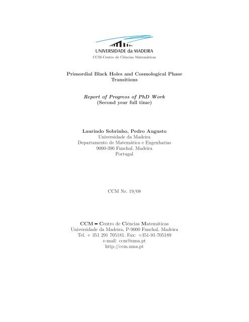
Figure 1: The time evolution of the abundances of the light elements produced
during Primordial Nucleosynthesis. It is also shown the decrease of the neutron
abundance (adapted from Burles et al., 1999).
reaction could then proceed with the formation of 3 1H (tritium), 3 2He, 4 2He, 6 3Li,
7
3Li and, 7 4Be. The reason why Primordial Nucleosynthesis did not progress
to produce elements with higher mass numbers is due to two factors: i) the
temperature of the universe which is by this time lower than required and,
ii) there are no stable nuclides with mass number A = 5 or A = 8. When
the Universe become ∼ 1000 s old the formation of nuclides effectively ceased
leaving a Universe with primary matter content of hydrogen (mainly protons,
i.e., 1 1H) and helium (mainly 4 2He), with trace amounts of beryllium and lithium
(e.g. Jones & Lambourne, 2004, Figure 1).
The radiation and matter densities in the Universe decrease as the expansion
dilutes the number of atoms and photons. Radiation also decreases due to the
cosmological redshift (see equation 25), so its density falls faster than that of
matter. Looking back in time, there was an instant, which corresponds to an
age of the Universe of ∼ 104 years (redshift z ≈ 3200, e.g. Bennett et al., 2003;
Hinshaw et al., 2008), when matter and radiation densities were just equal (cf.
Table 1, Figure 2). Before that time the Universe was radiation–dominated.
At an age of ∼ 105 years the universe had expanded and cooled enough
(T ∼ 4000 K), allowing nuclei and electrons to combine in order to form neutral
atoms. This process, which is known as recombination 6 , can be numerically
defined as the instant in time when the number density of ions is equal to the
number density of neutral atoms (e.g. Ryden, 2003).
6 Some authors suggest that we should use the term combination instead because this is
the very first time in the history of the universe when electrons and ions combined to form
neutral atoms (e.g. Ryden, 2003).

PBHs and Cosmological Phase Transitions 12
Figure 2: The energy densities of matter and radiation as a function of the
scale factor R(t). At a time when R(t)/R(t0) ≈ 10 −4 the energy densities of
matter and radiation were equal (R(t0) represents the present day value of the
scale factor). It is also represented the energy density due to the cosmological
constant, which does not vary with redshift, and is exceeded by the energy
densities in matter and radiation at early times (e.g. Jones & Lambourne, 2004).
When the universe was ∼ 380000 years old (z ≈ 1090, e.g. Bennett et al.,
2003; Hinshaw et al., 2008) and the temperature had dropped to ∼ 3000 K, the
number density of free electrons was so low that the universe essentially became
transparent and photons could travel unhindered from this time on. This
is known as the photon decoupling epoch. The photons released during this
epoch become the CMB (Section 1.7). Surrounding every observer in the universe
there is a last scattering surface from which the CMB photons have been
streaming freely (e.g. Ryden, 2003) becoming redshifted due to the expansion
of the universe (Section 1.7).
The period between photon decoupling (z ≈ 1090) and the formation of the
first luminous objects (z ∼ 11) is referred to as the Cosmic Dark Ages. That is
because, during that period, there were no sources of radiation in the Universe,
with the exception of the hyperfine 21–cm line of neutral hydrogen (e.g. Hirata
& Sigurdson, 2007).
Reionization is the second of two major phase changes of hydrogen gas in
the Universe (the first was recombination). Reionization occurred once objects
started to form in the early Universe, which was energetic enough to ionize
neutral hydrogen. As these objects formed and radiated energy, the Universe
went from being neutral back to being an ionized plasma, at redshift z ∼ 11
according to WMAP (Wilkinson Microwave Anisotropy Probe) results (Hinshaw
et al., 2008).
When the universe was ≈ 2.8 × 10 17 s old (≈ 0.7 times the present age) it
become dark energy–dominated (see Figure 2). The true nature of this dark

PBHs and Cosmological Phase Transitions 13
energy, which is responsible for the observed non–linear acceleration of the universe,
remains unknown (Section 1.8).
In Table 1 we present a timeline of the Universe according to the inflationary
Big Bang model.
1.3 Inflation
In order to explain problems such as ‘flatness’, ‘horizon’ and ‘monopole’ the
present paradigm makes use of an inflationary stage of expansion in the very
early Universe. During inflation the scale factor R(t) behaves like (e.g. Narlikar
& Padmanabhan, 1991)
R(t) =R(ti) exp (H(t − ti)) . (38)
The scale factor grows exponentially from an initial value Ri = R(ti), corresponding
to the instant ti ∼ 10 −35 s when the EW and strong forces separate
(e.g. Narlikar & Padmanabhan, 1991, cf. Table 1) to a value Re = R(te) according
to (e.g. d’Inverno, 1993)
Re
Ri
= e N(te)
where (e.g. Tsujikawa, 2003)
N(te) = ln Re
Ri
=
tf
ti
Hdt ≈ Hte
(39)
(40)
gives the number of e–folds that elapsed during inflation. For example, the
value N = 70 means that during inflation the scale factor have grown up by a
factor of e 70 (≈ 10 30 ). Although the exact value of N(te) is unknown, in order
to solve the mentioned problems, the inflationary stage must last a time interval
such that 50 0
which means that the R 2 H 2 term in equation (31) increases during inflation.
As a result Ω rapidly approaches unity (see equation 36). After the inflationary
period, the evolution of the Universe is followed by the conventional Big Bang
phase (Section 1.2) and, despite this, Ω stays of order unity even in the present
epoch, solving the flatness problem (e.g. Tsujikawa, 2003).
Inflation gives rise to a remarkable phenomenon: physical wavelengths grow
faster than the size of the Hubble radius (see equation 28). This means that
the region where the causality works is stretched on scales much larger than
the Hubble radius, i.e., once a physical wavelength becomes larger than the
Hubble radius, it is causally disconnected from physical processes. This solves
the horizon problem (e.g. Boyanovsky et al., 2006). Notice that Inflationary
cosmology suggests that, even though the observed Universe is incredibly large,
it is only an infinitesimal fraction of the entire Universe (e.g. Guth, 2000).

PBHs and Cosmological Phase Transitions 14
Table 1: The Universe timeline according to the inflationary Big Bang model
(data was taken mainly from Unsöld & Bascheck (2002) and Jones & Lambourne
(2004).
Era t(s) T (K) T (GeV) Comments
Planck – – – Quantum Gravity
GUT 10 −43 10 32 10 19 Gravity separates
Quark 10 −35 10 27 10 14 Strong–electroweak
phase transition
Inflation begins
∼ 10 −33 10 27 10 14 Inflation ends
3 × 10 −11 172.5 t quark threshold
2.3 − 3.2 × 10 −10 10 15 100 EW phase transition
10 −8 4.2 b quark threshold
10 −7 1.78 Lepton τ threshold
1.25 c quark threshold
1.6 − 1.2 Hyperons threshold
1.2 × 10 −5 0.50 Kaons threshold
Hadron 0.63 − 1.1 × 10 −4 10 13 0.17 Formation of neutrons
and protons
1.6 × 10 −4 0.14 Pions threshold
2.8 × 10 −4 0.106 Muons threshold
Lepton 3.5 × 10 −4 10 12 s quark threshold
and last pions decay
1 10 10 Decoupling of νe
2 Neutron production
stops
Photon 3 7.3 × 10 9 5 × 10 −4 Electron threshold
200 10 9 Nucleosynthesis of 2 H
stable
10 3 Nucleosynthesis stops
Matter 2.5 × 10 12 Radiation–Matter
equality
9.0 × 10 12 4000 Recombination
1.2 × 10 13 3000 Photon decoupling
1.1 × 10 16 30 Reionization
Λ 2.8 × 10 17 ≈ 4 Matter–Dark energy
equality
4.3 × 10 17 2.725 Present

PBHs and Cosmological Phase Transitions 15
Inflation is, perhaps, the simplest known mechanism to eliminate monopoles
from the visible Universe, even though they are still in the spectrum of possible
particles. The monopoles are eliminated simply by arranging the parameters so
that inflation takes place after (or during) monopole production, so the monopole
density is diluted to a completely negligible level (e.g. Guth, 2000).
The inflationary era is followed by the radiation–dominated and matter–
dominated stages where the acceleration of the scale factor becomes negative.
With a negative acceleration of the scale factor, the Hubble radius grows faster
than the scale factor, and wavelengths that were outside, can now re–enter the
Hubble radius. This is the main concept behind the inflationary paradigm for
the generation of temperature fluctuations as well as for providing the seeds for
Large Scale Structure (LSS) formation (e.g. Boyanovsky et al., 2006).
The basic ingredient for structure formation is the presence of initial density
fluctuations, that can, in a later time, act as seeds for the gravitational collapse.
Once a small overdensity appears, gravity causes it to grow and finally collapse
into a bounded system. As a result we have an inhomogeneous Universe on
small scales (e.g. Covi, 2003).
The density fluctuations cannot grow while the pressure of the plasma counteracts
the gravitational force and, therefore, during the radiation era the system
is still in the linear regime and only oscillations in the plasma (the so called
acoustic peaks) take place. Later, when matter dominates, the pressure drops to
zero and the fluctuations can grow: structures start to form and, consequently,
the complicated non–linear regime begins (e.g. Covi, 2003).
Inflation gives a possible solution to the crucial problem of where the primordial
fluctuations leading to the observed LSS come from. In fact, they have
their origin in the ubiquitous vacuum fluctuations. The seed of the LSS has
been observed in the form of tiny fluctuations imprinted on the CMB at the
time of decoupling (e.g. Bringmann et al., 2002).
There are various inflationary scenarios (e.g. slow roll inflation, old inflation,
new inflation, chaotic inflation, hybrid inflation, viscous inflation, tepid inflation,
natural inflation, supernatural inflation, extranatural inflation, eternal inflation,
extended inflation) differing essentially only in the choice of the potential V (φ)
where φ represents the inflaton, i.e., the scalar field responsible for inflation (e.g.
Boyanovsky et al., 2006). Each inflationary model makes precise predictions
about the spectrum of its primordial fluctuations and this is how these models
can be constrained by observations (e.g. Bringmann et al., 2002).
These different kinds of models can be roughly divided into three types (e.g.
Tsujikawa, 2003): Type I: large field model, in which the initial value of the
inflaton is large and rolls down to the potential minimum at smaller φ. Chaotic
inflation is one of the representative models of this class (see Figure 3); Type II:
small field model, in which the inflaton field is small initially and slowly evolves
toward the potential minimum at larger φ. New inflation and natural inflation
are the examples of this type (see Figure 4); Type III: hybrid (double) inflation
model, in which inflation typically ends by the phase transition triggered by the
presence of a second scalar field or by the second phase of inflation after the
phase transition (see Figure 5).

PBHs and Cosmological Phase Transitions 16
Figure 3: The schematic illustration of the potential of the chaotic inflation
model. This belongs to the class of the large field model (Tsujikawa, 2003;
Guth, 2000).
Figure 4: The schematic illustration of the potential of the natural inflation
model which belongs to the class of the small field model. Here f represents the
width of the inflaton potential (tipically f ∼ mP ∼ 10 19 GeV). When φ = πf
the potential vanishes (Tsujikawa, 2003).

PBHs and Cosmological Phase Transitions 17
Figure 5: The schematic illustration of the potential of the hybrid (double)
inflation model. This model is characterized by multiple scalar fields. In this
example we have two scalar fields: φ and χ. For large φ we have a situation similar
to the other models with a single field. However, when φ reaches the critical
value φc a different behaviour takes place. In particular, the energy density
during inflation can be much lower than normal while still giving suitably large
density perturbations, and secondly the field φ can be rolling extremely slowly
which is of benefit to particle physics model building (Liddle, 1999; Tsujikawa,
2003).
The inflaton φ is an homogeneous scalar field, whose potential energy V (φ)
leads to the exponential expansion of the Universe. The number of e–folds that
elapsed during inflation (equation 40) can be written also as a function of φ
(e.g. Boyanovsky et al., 2006)
N(φ(t)) = − 1
m 2 pl
φe
φ(t)
V (φ)
V ′ dφ. (41)
(φ)
The energy density and the pressure density of the inflaton can be described,
respectively, as (e.g. Liddle & Lyth, 1993)
ρ = 1
2 ˙ φ 2 + V (φ) (42)
p = 1
2 ˙ φ 2 − V (φ). (43)
Substituting equations (42) and (43) for equations (2) and (4) we get (e.g. Liddle
& Lyth, 1993) 7
H 2 = 8πG
3
1
2 ˙ φ 2
+ V (φ) = 8π
3m2
1
pl 2 ˙ φ 2
+ V (φ)
(44)
7 We have written equation (44) also in terms of the Planck mass mpl =(c/G) 1/2 with
= c = 1.

PBHs and Cosmological Phase Transitions 18
¨φ +3H ˙ φ + V ′ (φ) = 0 (45)
where we have considered κ = 0 and Λ = 0 in equation (44). Here, the prime
denotes the derivative of the potential with respect to the inflaton field.
Amongst the wide variety of inflationary scenarios, slow roll inflation provides
a simple and generic description of inflation consistent with the WMAP
data (e.g. Boyanovsky et al., 2006). The basic premise of slow roll inflation is
that the potential is fairly flat during the inflationary stage. This flatness not
only leads to a slowly varying inflaton and Hubble parameter, hence ensuring a
sufficient number of e–folds, but also provides an explanation for the gaussianity
of the fluctuations as well as for the almost scale invariance of their power spectrum.
Departures from scale invariance and gaussianity are determined by the
departures from flatness of the potential, namely by derivatives of the potential
with respect to the inflaton field (e.g. Boyanovsky et al., 2006). The slow roll
approximation corresponds to (e.g. Carr, 2005)
ξ ≪ 1, |η| ≪ 1 (46)
where ξ and η are the so called slow–roll parameters which are determined by
the derivatives of the inflaton potential in the following manner (e.g. Carr, 2005)
ξ = m2 pl
16π
V ′
V
2
(47)
η = m2pl V
8π
′′
. (48)
V
The inflationary era ends when ξ and |η| grow to order unity (e.g. Tsujikawa,
2003). At that time the scalar field starts to roll faster and finally to oscillate
around the minimum and finally it decays producing radiation and reheating
the Universe (e.g. Covi, 2003). If the conditions (46) are valid then equations
(44) and (45) are approximately given by (e.g. Boyanovsky et al., 2006)
H 2 = 8π
3m2 V (φ) (49)
pl
3H ˙ φ + V ′ (φ) = 0. (50)
Inflation is now an established part of Cosmology with several important aspects,
such as the superhorizon origin of density perturbations, having been
spectacularly validated by WMAP (e.g. Boyanovsky et al., 2006). The gaussian
and nearly scale invariant spectrum of primordial fluctuations generically predict
by most inflationary models fits with high precision the data provided by
WMAP (e.g. Spergel et al., 2007).
1.4 Cosmological phase transitions
The inflationary stage is followed by a radiation–dominated era after a short
period of reheating during which the energy stored in the inflaton field decays

PBHs and Cosmological Phase Transitions 19
into quanta of many other fields, which, through scattering processes, reach a
state of local thermodynamic equilibrium. This period is followed by deccelerated
expansion and cooling, with the Universe successively visiting the different
energy scales at which particle and nuclear physics predict symmetry breaking
phase transitions. Those phase transitions are broadly characterized as either
second or first–order (e.g. Boyanovsky et al., 2006).
If a thermodynamic quantity changes discontinuously (for example as a function
of temperature) we have a first–order phase transition. This happens because,
at the point at which the transition occurs, there are two separate thermodynamic
states in equilibrium. Any thermodynamic quantity that undergoes
such a discontinuous change at the phase transition is referred to as an order
parameter. Whether or not a first–order phase transition occurs often depends
on other parameters that enter the theory. It is possible that, while another
parameter is varied, the change in the order parameter of the phase transition
decreases until they, together with all other thermodynamic quantities, become
continuous at the transition point. In this case we refer to a second order phase
transition at the point at which the transition becomes continuous (i.e., it shows
a thermodynamic behaviour without discontinuities or singularities in the free
energy or any of its derivatives), and a continuous crossover at the other points
for which all physical quantities undergo no changes (e.g. Trodden, 1999). However,
if the crossover is relatively sharp the situation may not be too different
from a phase transition (e.g. Boyanovsky et al., 2006).
Phase transitions are the most important phenomena in particle cosmology
since, without them, the history of the Universe would simply be one of gradual
cooling. In the absence of phase transitions, the only departure from thermal
equilibrium is provided by the expansion of the Universe (e.g. Trodden, 1999).
The SMPP (Section 1.8) predicts two phase transitions. The first one, at
temperatures of ∼ 100 GeV, is the Electroweak phase transition (Section 3)
which was responsible for the spontaneous breaking of the EW symmetry, which
gives the masses to the elementary particles. This transition is also related to
the EW baryon–number violating processes, which had a major influence on the
observed baryon–asymmetry of the Universe (e.g. Aoki et al., 2006b).
The second transition occurs at T ≈ 170 MeV. It is related to the spontaneous
breaking of the chiral symmetry of the Quantum Chromodynamics (QCD)
when quarks and gluons become confined in hadrons (Section 2). At high temperatures
asymptotic freedom of QCD predicts the existence of a deconfined
phase (according to lattice QCD simulations), the Quark–Gluon Plasma (QGP).
At low temperatures quarks and gluons are confined in a Hadron Gas (HG) (e.g.
Schmid et al., 1999).
The QCD phase transition was pointed out, for a long time, as a prime candidate
for a first–order phase transition (e.g. Jedamzik & Niemeyer, 1999). Recent
results (e.g. Aoki et al., 2006b) provide strong evidence that the QCD transition
is a simple Crossover instead. Here we will consider the two possibilities (see
Section 2).

PBHs and Cosmological Phase Transitions 20
1.5 The Lambda–Cold Dark Matter Model
In the last few years there has been a wealth of observational evidence from
CMB, LSS and high redshift supernovae Ia data that leads to the remarkable
conclusions that: i) the spatial geometry of the Universe is flat (κ = 0), ii) the
Universe is accelerating today, and iii) most of the matter is in the form of
dark matter. The current understanding of cosmology is based on the so called
Lambda–Cold Dark Matter Model (ΛCDM) in which the total energy density
of the Universe has as main ingredients: 5% of baryonic matter, 25% of dark
matter and 70% of dark energy (e.g. Boyanovsky et al., 2006).
Baryonic matter
Ordinary matter is mainly composed of protons and neutrons (which are baryons)
and electrons (which are leptons). Since the baryons vastly outweigth the electrons,
in the context of Cosmology, ordinary matter is called baryonic matter
(e.g. Lyth, 1993). The luminous matter in the Universe accounts for only
Ωb ≈ 0.042 (Spergel et al., 2007) which means that there exists a great amount
of baryonic dark matter in the Universe. This discrepancy is refered as the
missing matter problem (e.g. d’Inverno, 1993).
Within a galaxy, baryons are expected to concentrate more in the central
luminous part than in the dark halo. The reason is that baryons (electrons
included) can emit radiation whereas non–baryonic dark matter interacts too
weakly to do so (or it would not be dark). Baryons lose more energy, allowing
them to settle more deeply into the galaxy centre. Baryons within galaxies could
be in the form of non–emitting gas, failed stars or planets, (∼ 0.01 − 0.1M⊙),
and dead stars (old white dwarfs, non–emitting neutron stars and black holes).
In the intergalactic space, baryons can only be in the form of non–emitting gas
because, as far as we know, bound objects form only within galaxies (e.g. Lyth,
1993) or within galaxy clusters.
Non–Baryonic Dark Matter
If Ωm ≈ 0.24 as measured by WMAP (Spergel et al., 2007) then, besides baryonic
matter (luminous and dark), there might exist a huge amount of non–
baryonic dark matter (e.g. Lyth, 1993).
We can estimate the total amount of matter in a bound system, such as a
galaxy or galaxy cluster, through its gravitational field, which can be deduced
from the velocities of its components. One finds that each galaxy is surrounded
by a dark halo accounting for most of its mass (e.g. Lyth, 1993).
Soon after the need for dark matter came to be widely accepted in the early
1980s, it became clear that the hypothesis fails completely if the dark matter
consists of massive neutrinos, because their thermal motion wipes out small
scale structure. Given the failure of this Hot Dark Matter (HDM) model, attention
turned to the other extreme, of matter which has, by definition, negligible
random motion. In its standard form, the Cold Dark Matter (CDM) model
assumes that the Universe has a flat spatial geometry, a critical matter density

PBHs and Cosmological Phase Transitions 21
(see equation 32) and a spectrum which is precisely scale invariant (e.g. Liddle
& Lyth, 1993).
As implied by its name, the CDM is assumed to be cold, which, for most
purposes, means non–relativistic. By definition, dark matter does not interact
significantly with more conventional forms of matter by any means other than
gravity, and, in particular, is beneficial for structure formation in that it is not
subject to pressure forces from interaction with radiation which prevent baryonic
density inhomogeneities on scales smaller than superclusters from collapsing
before radiation decouples from matter. Structure can, thus, start to form earlier
within dark matter, providing initial gravitational wells to kick–start structure
formation within baryonic matter after decoupling (e.g. Liddle & Lyth, 1993).
The current best candidate for CDM are the so–called weakly interacting
massive particles (WIMPs) that might have been produced in the very early
Universe (e.g. Bertone et al., 2005).
Dark energy
Independent measurements of Type Ia supernovae have revealed that the expansion
of the Universe is undergoing a non–linear acceleration rather than
following strictly Hubble’s law. To explain this acceleration, general relativity
requires that much of the Universe consist of an energy component with large
negative pressure. Its true nature remains unknown, although the present observations
indicate that this dark energy can be described by a cosmological
constant Λ (e.g. Boyanovsky et al., 2006).
The model assumes a nearly scale–invariant spectrum of primordial perturbations
and a Universe without spatial curvature (k =0⇒ Ωκ = 0). It also
assumes that it has no observable topology, so that the Universe is much larger
than the observable particle horizon. Those are predictions of cosmic inflation
(Section 1.3).
The ΛCDM model has six parameters: the Hubble constant H0, the baryon
density Ωb, the total matter density Ωm (which includes baryons plus dark
matter), the optical depth to reionization τ (which determines the redshift of
reionization), the amplitude of the primordial fluctuations As and the slope for
the scalar perturbation spectrum ns (which measures how fluctuations change
with scale; ns = 1 corresponds to a scale–invariant spectrum). The values of
these six free parameters as obtained from the WMAP data (Spergel et al.,
2007) are presented in Table 2. The Hubble constant h is given in normalized
units of 100 kms −1 Mpc −1 and the densities Ωm and Ωb are given as functions
of h. Thus, the present value of the Hubble parameter H0 is, according to the
most recent WMAP observations
and
H0 = 73.4 kms −1 Mpc −1 ≈ 2.38 × 10 −18 s −1
(51)
Ωm ≈ 0.24 (52)

PBHs and Cosmological Phase Transitions 22
Table 2: The best fit values for the ΛCDM model free parameters according to
the WMAP data (Spergel et al., 2007).
Parameter Value Description
h 0.734 +0.028
−0.038
100Ωbh 2 2.233 +0.072
−0.091
Ωmh 2 0.1268 +0.0072
−0.0095
τ 0.088 +0.043
−0.054
As
ns
0.801 +0.043
−0.054
0.951 +0.015
−0.019
Normalized Hubble constant
Baryon density
Total matter density
Optical depth to reionization
Scalar fluctuation amplitude at k =0.002 Mpc −1
Scalar spectral index at k =0.002 Mpc −1
Ωb ≈ 0.042. (53)
Notice that the dark energy density ΩΛ (cf. equation 35) is not a free parameter
because, since the ΛCDM model assumes a flat Universe (Ω = 1), we have,
according to equation (36)
ΩΛ =1− Ωm ≈ 0.76. (54)
Other derived parameters are the age of the Universe t0 (Section 1.6) and the
critical density ρ0 (cf. equation 32). Inserting the value of H0 into equation
(32) one obtains
ρc = ρ0 ≈ 1.013 × 10 −26 kgm −3 . (55)
The cosmological constant, which is also a derived parameter, is given by (see
equations 32 and 35)
Λ= 8πG
c 2 ρΛ = 8πG
c 2 ΩΛρc = 3H2 0 ΩΛ
c 2 . (56)
Inserting the obtained values for H0 (equation 51) and ΩΛ (equation 54) into
equation (56) one obtains 8
Λ ≈ 1.44 × 10 −52 m −2 . (57)
8 When one calculates the theoretical value of Λ one ends up with a value about 120 orders
of magnitude larger than the experimentally measured one. This has been called the worst
mismatch between theory and experiment in the whole of science (e.g. Weinberg, 2000).

PBHs and Cosmological Phase Transitions 23
The expansion of the Universe is sometimes described by means of a deceleration
parameter q which is defined as (e.g. d’Inverno, 1993)
q(t) =− R ¨ R
˙R 2 = − ¨ R
RH 2
(58)
where q>0 means that the expansion is slowing down and q0) only if Ωm > ΩΛ. However it is usual to retain the historical
deceleration parameter designation even when q

PBHs and Cosmological Phase Transitions 24
When the Universe becomes dominated by dark energy (Λ > 0) the Hubble
parameter becomes constant in time (cf. expression 19)
Λ
H(t) =c . (65)
3
Since inflation only lasts a few e–folds (see Section 1.3), the Hubble parameter
can be taken as a constant during this period (e.g. Huang, 2007; Narlikar &
Padmanabhan, 1991). From equation (40) we have
H(t) = N(te)
. (66)
te
Considering the normalisation (61) we can determine the proportionality constant
in expression (19), yielding, for the scale factor of a Universe dominated
by a positive cosmological constant, the result 9
R(t) = exp c
Λ
3
(t − t0) , tSN ≤ t ≤ t0 (67)
where t0 is the present time (i.e. the age of the Universe) and tSN is the age
of the universe at matter–Λ equality (corresponding to the instant when the
expansion starts to accelerate). The dark energy domination is preceded by a
matter–dominated stage which started when photons decoupled from matter.
During matter domination the scale factor behaves according to expression (18).
Considering that R(t) is a continuous function of time we will write, for the
matter–dominated stage
Λ
R(t) = exp c 3 (tSN
2/3 t − t0)
, teq ≤ t ≤ tSN (68)
tSN
where teq is the age of the Universe at radiation–matter equality. Before that
time, the Universe was radiation–dominated up to the end of inflation at some
instant t = te. During radiation domination the scale factor behaves according
to expression (17). During the period (te ≤ t ≤ teq) the Universe experienced
two phase transitions during which it might have been, for brief instants, dust–
like (Section 2). When one goes backwards in time the first phase transition
is the QCD. Considering that t+ corresponds to the age of the Universe at the
end of the QCD we write
Λ
R(t) = exp c 3 (tSN
2/3 1/2 teq t
− t0)
, t+ ≤ t ≤ teq (69)
tSN teq
9 To our best knowledge, this sequence of formulae (equations 67–77) has never been deducted
in the literature, although common-knowledge.

PBHs and Cosmological Phase Transitions 25
We consider that during the QCD epoch (t− ≤ t ≤ t+) the scale factor is given
by
Λ
R(t) = exp c
3 (tSN
2/3 1/2 teq t+
− t0)
×
nqcd t
× ,t− ≤ t ≤ t+
t+
tSN
teq
(70)
where nqcd =2/3 if the Universe experiences a dust–like phase during the QCD
and nqcd =1/2 if the Universe continues to be radiation–dominated during that
epoch. Between the end of the EW transition (t = tEW+) and the beginning of
the QCD phase transition (t = t−) the Universe is radiation–dominated. Thus,
we write
Λ
R(t) = exp c
3 (tSN
2/3 1/2 nqcd teq t+ t−
− t0)
×
1/2 t
× ,tEW+ ≤ t ≤ t−
t−
tSN
teq
t+
(71)
During the EW transition (tEW− ≤ t ≤ tEW+) we consider that the scale factor
is given by
Λ
R(t) = exp c
3 (tSN
2/3 1/2 nqcd teq t+ t−
− t0)
×
×
tEW+
t−
1/2 t
tEW+
new
tSN
teq
,tEW− ≤ t ≤ tEW+
t+
(72)
where new =2/3if the Universe experiences a dust–like phase during that epoch
and new =1/2 if the Universe continues to be radiation–dominated. Between
the end of inflation (t = te) and the beginning of the EW phase transition
(t = tEW−) the Universe is radiation–dominated. We write
Λ
R(t) = exp c
3 (tSN
2/3 1/2 nqcd teq t+ t−
− t0)
×
×
tEW+
t−
tSN
1/2 new
tEW− t
tEW+
tEW−
teq
1/2
t+
,te ≤ t ≤ tEW−
(73)
During inflation the scale factor behaves according to expression (38). Thus, at
the end of the inflationary period the scale factor can be written as
R(te) =R(ti) exp (Hi(te − ti)) . (74)

PBHs and Cosmological Phase Transitions 26
On the other hand we have, from equation (73)
Λ
R(te) = exp c
3 (tSN
2/3 1/2
teq t+ t−
− t0)
×
tEW+
t−
tSN
1/2 new
tEW− te
tEW+
tEW−
teq
1/2
.
t+
nqcd
×
(75)
Combining equations (74) and (75) one finds an expression for R(ti). Inserting
this expression into equation (38) one obtains, for the scale factor during
inflation, the result
Λ
R(t) = exp c
3 (tSN
2/3 1/2 nqcd teq t+ t−
− t0)
×
×
tEW+
t−
tSN
1/2 new
tEW− te
tEW+
× exp (Hi (t − ti))
exp (Hi (te − ti)) ,ti ≤ t ≤ te
tEW−
teq
1/2
×
t+
(76)
where Hi corresponds to the value of the Huble parameter during inflation that
we assume constant (cf. equation 66). Finally, considering that before inflation
the Universe is radiation–dominated, we write
Λ
R(t) = exp c
3 (tSN
2/3 1/2 nqcd teq t+ t−
− t0)
×
×
tEW+
t−
tSN
1/2 new
tEW− te
tEW+
tEW−
teq
1/2
×
1/2 t
× exp (−Hi (te − ti)) ,tp ≤ t ≤ ti
ti
t+
(77)
where tp represents the Planck time.
The scale factor R, the background temperature T and the redshift z at a
given epoch are related according to the expression (e.g. Unsöld & Bascheck,
2002)
T (t)
T0
= R0
= 1 + z (78)
R(t)
where T0 represents the present day background temperature (T0 ≈ 2.725).

PBHs and Cosmological Phase Transitions 27
The value of t0, i.e., the age of the Universe, can be obtained with the help
of expression (e.g. Yao et al., 2006)
H0t0 =
∞
0
dz
. (79)
(1 + z)H(z)
In the case of a flat Universe (Ωm +ΩΛ = 1) expression (79) can be written as
(e.g. Yao et al., 2006)
H0t0 = 2
3 √ ΩΛ
ln 1+√ΩΛ √ , Ωm < 1. (80)
1 − ΩΛ
Inserting H0 (see equation 51) into equation (80) with ΩΛ =0.76 we obtain, for
the age of the Universe
t0 ≈ 4.3 × 10 17 s. (81)
Considering that during the cosmological constant domination the Hubble parameter
stays constant (cf. equation 65) we have that H(tSN) =H0. Thus,
inserting H0 into equation (64) we obtain
tSN ≈ 2.8 × 10 17 s. (82)
Notice that if Λ = 0 this would correspond to t0. This means that, in the
absence of dark energy, the Universe would be younger by a factor of ≈ 1.5 (e.g.
Jones & Lambourne, 2004).
The value of teq can be obtained with the help of equations (62) and (68)
considering that z ≈ 3200 at radiation–matter equality (e.g. Hinshaw et al.,
2008)
teq ≈ 2.5 × 10 12 s. (83)
Proceding the same way, one obtains, for the age of the universe at photon
decoupling (z ≈ 1090)
tdec ≈ 1.2 × 10 13 s. (84)
Taking ti = 10 −35 s we have, from equations (63) and (66), that
te ∼ 10 −33 s (85)
valid for both N(te) = 50 and N(te) = 70.
The calculus of numerical values to t−, t+, tEW− and tEW+ will be discused
in Sections 2.4 and 3.2. For the moment, we present on Table 3 all these instants
of time as well as the corresponding values for the scale factor. Notice that some
of these values may be slightly different, depending on the values one chooses
for nqcd, new and t−.
In Figure 6 we show R(t) during the QCD transition. Notice that the reduction
on the scale factor during a dust–like QCD transition is not very significative.
In fact the term t−/t+ is ∼ 1 and, thus, it can be neglected in equations

PBHs and Cosmological Phase Transitions 28
(71) to (77). Notice, however, that this will not be the case if one is working
locally (i.e., near t− and t+). In Section 2.4, for example, we want to determine
numerical values for t− and t+. In that case, it does not make sence to consider
t−/t+ = 1. The same idea is valid for the term tEW−/tEW+. According to this,
we can replace equations (69) to (73) by the single equation
Λ
R(t) = exp c 3 (tSN
2/3 1/2 teq t
− t0)
, te≤t≤ teq (86)
tSN teq
Equations (67) and (68) remain unchanged. Equation (76) becomes
Λ
R(t) = exp c
3 (tSN
2/3 1/2 teq te
− t0)
and equation (77) becomes
tSN
teq
exp (Hi (t − ti))
exp (Hi (te − ti)) ,ti ≤ t ≤ te
Λ
R(t) = exp c 3 (tSN
2/3 1/2 teq te
− t0) tSN teq
1/2 t
exp (−Hi (te − ti)) ,tp ≤ t ≤ ti
ti
(87)
(88)
In Figure 7 we show R(t) for the entire Universe timeline (i.e., from the Planck
time tp up to the present time t0).
1.7 The Cosmic Microwave Background temperature
The existence of the Cosmic Microwave Background (CMB) radiation was first
predicted by Gamow et al. (1948) but it was only in 1964 that it was observed
(serendipitously) by the first time (Penzias & Wilson, 1965).
In 1989, NASA launched the Cosmic Background Explorer satellite (COBE),
and the initial findings, released in 1990, were consistent with the Big Bang’s
predictions regarding the CMB. COBE found a residual temperature of 2.726 K
and determined that the CMB was isotropic to about one part in 10 5 (Boggess
et al., 1992). During the 1990s, CMB anisotropies were further investigated
by a large number of ground–based experiments and the Universe was shown
to be almost geometrically flat, by measuring the typical angular size of the
anisotropies.
The CMB brings us information about the state of the Universe at the
photon decoupling epoch (z ≈ 1090) when the photons that reach us now had
their last scattering (Section 1.2). The spectrum of the CMB at the present
epoch is well described by a blackbody function with (e.g. Boyanovsky et al.,
2006)
T0 =2.725 ± 0.001K (89)

PBHs and Cosmological Phase Transitions 29
Table 3: The Scale Factor (equations 67–77) for different instants of time during
the evolution of the Universe: tp (Planck time), ti (beginning of inflation), te
(end of inflation), tEW− (beginning of the EW transition – Section 3.2), tEW+
(end of the EW transition – Section 3.2), t− (beginning of the QCD transition
– Section 2.4), t+ (end of the QCD transition – Section 2.4), teq (last scattering
surface), tSN (the instant when the Universe starts to accelerate) and t0 (present
time). Notice that we have indicated two values for t−. The first one corresponds
to the Bag Model results and the second one to the Lattice Fit results (cf.
Section 2.4).
t(s) R(t)
tp ∼ 10 −43 ∼ 10 −60
ti ∼ 10 −35 ∼ 10 −56
te ∼ 10 −33 ∼ 10 −27
tEW− 2.30 × 10 −10 2.9 × 10 −15
tEW+ 3.15 × 10 −10 3.5 × 10 −15
Log 10Rt
t− 6.25 × 10 −5 1.4 × 10 −12 (QCD Bag)
t− 9.35 × 10 −5 1.9 × 10 −12 (QCD Lattice)
t+ 1.08 × 10 −4 2.1 × 10 −12
teq 2.5 × 10 12 3.2 × 10 −4
tSN 2.8 × 10 17 0.73
t0 4.3 × 10 17 1
-11.6
-11.7
-11.8
-11.9
QCD
-4.4 -4.3 -4.2 -4.1 -4 -3.9 -3.8 -3.7
Log 10t1s
Figure 6: The scale factor during the QCD transition as a function of time.
The gray region corresponds to the dust–like epoch, according to the Bag Model
(Sections 2.3.1 and 2.4). The curves correspond, from top to bottom, to the:
crossover case (nqcd =1/2), Lattice Fit (nqcd =2/3 and t− =9.35 × 10 −5 s)
and Bag Model (nqcd =2/3 and t− =6.25 × 10 −5 s).

PBHs and Cosmological Phase Transitions 30
Log 10Rt
0
-10
-20
-30
-40
-50
-60
Inflation EW QCD
-40 -30 -20 -10 0 10
Log 10t1s
matter
Figure 7: The scale factor as a function of time. The gray regions corresppond to
the inflationary period, the EW and QCD transitions and the matter–dominated
era. In blue (right side) we have the dark energy dominated era. The other
regions (in white) correspond to radiation–dominated periods.
Another observable quantity inherent in the CMB is the variation in temperature
(or intensity) from one part of the microwave sky to another. Since the first
detection of these anisotropies by the COBE satellite in 1992, there has been
intense activity to map the sky at increasing levels of sensitivity and angular
resolution. Observations have shown us that the CMB contains anisotropies at
the 10 −5 level (e.g. Yao et al., 2006)
∆T
T
∼ 10−5
(90)
over a wide range of angular scales. Density fluctuations over the plasma in thermal
equilibrium gave rise to temperature fluctuations (denser regions were hotter).
Hence, the temperature anisotropies in the CMB bring us direct evidence
of the density contrast at recombination. This small temperature anisotropy,
whose existence is predicted by cosmological models, provides the clue to the
origin of structure and is an important confirmation of theories of the early
Universe (e.g. Boyanovsky et al., 2006).
These anisotropies are usually expressed by using a spherical harmonic expansion
of the CMB sky (e.g. Yao et al., 2006)
T (θ, φ) =
almYlm(θ, φ) (91)
l,m
where Ylm(θ, φ) is the so–called spherical harmonic function of degree l and
order m 10 .
10 Ylm(θ, φ) represents the angular part of the solution of Laplace’s equation
(∇ 2 f(r, θ, φ) = 0). The degree l and order m are integers such that l ≥ 0 and |m| ≤ l.
The coefficients alm are constants. The expansion is exact as long as l goes to infinity.

PBHs and Cosmological Phase Transitions 31
Theoretical models generally predict that the alm modes are Gaussian random
fields. Tests show that this is an extremely good simplifying approximation,
with only some relatively weak indications of non–Gaussianity or statistical
anisotropy at large scales. With the assumption of Gaussian statistics, and if
there is no preferred axis, then it is the variance of the temperature field which
carries the cosmological information, rather than the values of the individual
alm coefficients. In other words, the power spectrum in l fully characterizes the
anisotropies (e.g. Yao et al., 2006).
On small sections of the sky where its curvature can be neglected, the spherical
harmonic analysis becomes ordinary Fourier analysis in two dimensions and
l becomes the Fourier wavenumber. Since the angular wavelength θ =2π/l,
larger multipole moments correspond to smaller angular scales, with l ∼ 10 2
representing degree scale separations. In this limit the power spectrum is usually
displayed as (e.g. Hu & Dodelson, 2002)
∆T
T
2
= l(l + 1)
where (e.g. Yao et al., 2006)
2π Cl (92)
Cl ≡ 〈|alm| 2 〉. (93)
The CMB mean temperature of 2.725 K (cf. equation 89) can be regarded
as the monopole component (a00) of CMB maps. Since all mapping experiments
involve difference measurements, they are insensitive to this average level.
Monopole measurements can only be made with absolute temperature devices,
such as the Far–InfraRed Absolute Spectrophotometer (FIRAS) instrument on
the COBE satellite. Such measurements of the spectrum are consistent with a
blackbody distribution over more than three decades in frequency (e.g. Yao et
al., 2006).
The largest anisotropy is in the l =1dipole first spherical harmonic, with
amplitude 3.346 ± 0.017 mK. The dipole is interpreted to be the result of the
Doppler shift caused by the solar system motion relative to the nearly isotropic
blackbody field, as confirmed by measurements of the radial velocities of local
galaxies (e.g. Yao et al., 2006).
Excess variance in CMB maps at higher multipoles (l ≥ 2) is interpreted as
being the result of perturbations in the density of the early Universe, manifesting
themselves at the epoch of the last scattering of the CMB photons. In the hot
Big Bang picture, this happens at a redshift z 1090, with little dependence
on the details of the model (e.g. Yao et al., 2006).
In Figure 8 we show the theoretical CMB anisotropy power spectrum (according
to the standard ΛCDM model). Notice that the physics underlying the
Cl’s can be separated into four main regions: the ISW Rise (l 2), the Sachs–
Wolfe plateau (l 100), the acoustic peaks (100 l 1000) and the damping
tail (l 1000).
The horizon scale at photon decoupling corresponds to l ≈ 100. Anisotropies
at larger scales (l

PBHs and Cosmological Phase Transitions 32
Figure 8: The theoretical CMB anisotropy power spectrum, using a standard
ΛCDM model. The horizontal axis is logarithmic. Four regions, each covering
roughly a decade in l, are labeled as: the ISW Rise; Sachs–Wolfe Plateau;
Acoustic Peaks (numbers indicate the first, the second and, the third acoustic
peak); and Damping Tail. Also shown is the shape of the tensor (gravity wave)
contribution, with an arbitrary normalization (adapted from Yao et al., 2006).
the initial conditions. The combination of gravitational redshift and intrinsic
temperature fluctuations leads to
δT
T
1 δφ
3 c2 (94)
where δφ is the perturbation to the gravitational potential. This is usually
referred to as the Sachs–Wolfe effect. Assuming, in addition, a nearly scale–
invariant spectrum of density perturbations, then l(l + 1)Cl is almost constant
at large scales (l

PBHs and Cosmological Phase Transitions 33
in the temperature–polarization angular power spectrum at l ∼ 150 (Spergel et
al., 2007).
The recombination process is not instantaneous, giving a thickness to the
last scattering surface. This leads to a damping of the anisotropies at the highest
multipoles (l >1000), corresponding to scales smaller than that subtended by
this thickness. This effect leads to a cut off on the anisotropies for l 2000.
Also, gravitational lensing, caused by structures at low redshift (z ≪ 1000),
would have the effect of partially flatten the peaks, generating a power-law tail.
The WMAP data can reach the multipole l 900, up to the third acoustic peak
(see Figure 8). In order to extend to higher multipoles (including the Damping
Tail region), the WMAP team included in their analysis the data of other two
CMB ground–based experiments: the Arcminute Cosmology Bolometer Array
Receiver (ACBAR) and the Cosmic Background Imager (CBI) (e.g. Covi, 2003).
Information on the density contrast can also be obtained from the distribution
of galaxies in our Universe. The main assumption, in this case, is that
the visible matter follows the distribution of the invisible Dark Matter. Recent
surveys include the 2 degree Field Galaxy Redshift Survey (2dFGRS) which released
data on 221 414 galaxies with measured redshift (e.g. Colless et al., 2003;
Cole et al., 2005). An even larger survey is the Sloan Digital Sky Survey (SDSS).
Its 6 th release of data (Adelman–McCarthy et al., 2008) already contains a total
of 790 860 galaxies. From the distribution of the galaxies in the sky one
can obtain the two point correlation function and the density contrast power
spectrum (e.g. Covi, 2003).
Other ways to measure the density contrast rely on using photons of distant
objects as a probe of the intervening matter or gas densities. Lyman α forest
data measure the absorption lines in the spectra of distant quasars caused by
intergalactic hydrogen and estimate the cosmic gas distribution out to large
distances (e.g. Covi, 2003). On Figure 9 we show, as an example, the Lyman α
forest of quasar RD J030117 + 002025.
1.8 The Standard Model of Particle Physics
The combination of the QCD theory and the EW is known as the Standard Model
of Particle Physics (SMPP). The SMPP contains a finite number of parameters,
which are unrelated, at least within the context of the theory itself. The SMPP
is based on only two basic components: the fundamental quantum particles
and the concept of interactions between them. A more complete theory of
fundamental physics should explain the relationships among these parameters.
The ultimate goal would be to determine the values of the parameters from pure
mathematics, once the correct theory is discovered (e.g. Scott, 2006).
The current SMPP, experimentally tested with remarkable precision, describes
the theory of strong, weak and electromagnetic interactions as a gauge
theory 11 . The particle content is (see Figure 10): three families of quarks, three
11 In Physics, gauge theories are a class of physical theories based on the idea that symmetry
transformations can be performed locally as well as globally. Many powerful theories in
Physics (e.g. EW theory, Electrodynamics, QCD) are described by Lagrangians which are

PBHs and Cosmological Phase Transitions 34
Figure 9: The spectrum of quasar RD J030117 + 002025 with redshift z =
5.50. The Lyman α emission line has been shifted from the ultraviolet (1210˚A)
to the infrared (7860˚A) and the same happened to the absorption caused by
hydrogen clouds between us and the quasar, each at its own redshift (covering
∼ 5000 − 8000˚A in this plot): the Lyα forest (adapted from Stern et al., 2000).

PBHs and Cosmological Phase Transitions 35
Figure 10: The particle content of the SMPP (http://wwwsldnt.slac.stanford.edu)
as regards fundamental fermions and bosons. Since
there are eight different types of gluons (g), two W bosons and the (still
hypothetical) Higgs boson (H) – not shown – there are a total of 25 particles.
families of leptons, and 13 gauge bosons (i.e., particles that act as carriers of
the fundamental interactions): eight massless gluons, Z 0 , W ± ; the massless
photon; the (yet to be discovered) scalar Higgs (e.g. Boyanovsky et al., 2006).
These particles interact in only three ways: the electromagnetic interaction, the
weak interaction and the strong interaction. Note that gravity is left outside
the SMPP because we do not yet have a theory of quantum gravity.
The classification of fundamental particles is performed taking into account
certain properties such as the rest mass, the electric charge and the spin. The
spin must be an integer or an half–integer and is normally expressed in units
of . Quantum particles with integer spin are called bosons and quantum particles
with half–integer spin are called fermions. Fermions obey the Exclusion
Principle (identical fermions cannot be at the same state at the same time) but
bosons do not obey the Exclusion Principle.
A particle which does not react to the strong interaction is called a lepton
(see Table 4, Figure 10). In the SMPP six of the 12 fermions are leptons:
three electric charged particles (electron – e − , muon – µ − , tau – τ − ) and their
associated neutrinos (νe, νµ, ντ). The remaining six fermions are quarks –
particles which react to the strong interaction (see Table 5, Figure 10). Quarks
invariant under certain symmetry transformation groups. When they are invariant under a
transformation identically performed at every space–time point they are said to have a global
symmetry. Gauge theory extends this idea by requiring that the Lagrangians must possess
local symmetries which enable symmetry transformations in a particular region of space–time
without affecting what happens in another region. This requirement is a generalized version
of the Equivalence Principle of general relativity.

PBHs and Cosmological Phase Transitions 36
Table 4: The three lepton families of the SMPP. For each particle
it is indicated the respective electric charge e, spin s and
mass m (according to the Particle Data Group (PDG) results –
http://pdg.lbl.gov/2007/listings/contents listings.html, Yao et al., 2006). For
each charged lepton there is an anti–lepton with symmetric charge and the
same mass and spin (e.g, the anti–particle of the electron is the positron, e + ,
which is a particle with electric charge +1, spin 1/2 and mass 0.511 MeV. At
the present it is not known if neutrinos are their own anti–particles (that would
depend on the nature of the physics that gives them masses).
Family Lepton Symbol e s m(MeV)
1 electron e − −1 1/2 0.511
electron neutrino νe 0 1/2 < 2 × 10 −6
2 muon µ − −1 1/2 105.658
muon neutrino νµ 0 1/2 < 0.19
3 tau τ − −1 1/2 1776
tau neutrino ντ 0 1/2 < 18.2
come in six flavours (up – u, down – d, strange – s, charm – c, top – t, bottom
– b) and carry, besides a fractional electric charge, a colour charge. This colour
charge comes in three types: red, green and blue. This means that there are 18
different quarks (6 flavours × 3 colours).
The pairings (e, µe) and (u, d) form a family of fundamental particles (Figure
10). Most of the matter we see around us ultimately consists of this family
of four particles. It seems that most matter in the Universe requires representatives
from only this family of fundamental particles. Yet, for some reason, this
family is reproduced twice over (cf. Figure 10).
Bosons act as carrier particles of the fundamental forces (see Table 6). The
photon, γ, is the carrier of the electromagnetic interaction. It acts on any
particle that possesses electric charge. There are two carrier particles of the
weak interaction: the W boson and the Z boson. The W boson is electrically
charged and so, there are W + and W − bosons (antiparticles of each other). The
Z boson is electrically neutral (Z 0 ). The weak interaction acts on all particles
including neutrinos (the only interaction felt by neutrinos).
The boson responsible for the strong interaction is the gluon (g) which couples
to the colour charge. The gluon possesses himself a colour charge, i.e. gluons
are themselves subject to the strong force. They exchange gluons with other
gluons which allows the possibility of glueballs (bound states of ‘pure glue’) and

PBHs and Cosmological Phase Transitions 37
Table 5: The three quark families of the SMPP. For each particle it is indicated
the respective electric charge e, spin s and mass m (according to the PDG results
– http://pdg.lbl.gov/2007/listings/contents listings.html, Yao et al., 2006). For
each quark there is an anti–quark with symmetric charge and the same mass
and spin (e.g., the up antiquark, ū, is a particle with electric charge −2/3, spin
1/2 and mass 1.5 to 3 MeV).
Family Quark Symbol e s m(MeV)
1 up u 2/3 1/2 1.5 to 3
down d −1/3 1/2 3 to 7
2 strange s −1/3 1/2 95 (±25)
charm c 2/3 1/2 1250 (±90)
3 bottom b −1/3 1/2 4200 (±70)
top t 2/3 1/2 172500 (±2700)
Table 6: Fundamental Bosons within the SMPP. For each boson it is shown the
respective electric charge e, spin s and mass m (according to the PDG results
– http://pdg.lbl.gov/2007/listings/contents listings.html, Yao et al., 2006).
Interaction Boson Symbol q s m(MeV)
electromagnetic photon γ 0 1 0
weak W W − −1 1 80403
Z Z 0 0 1 91188
W W + +1 1 80403
strong gluon g 0 1 0

PBHs and Cosmological Phase Transitions 38
hybrid mesons (bound states of a gluon, quark and antiquark).
There are six types of gluons that can change the colour charge of a quark
(but not its flavour): red–antigreen, red–antiblue, green–antired, green–antiblue,
blue–antired, and blue–antigreen. For example, if a red quark interacts with a
red–antigreen quark then it will become a green quark. In addition, there are
two different gluons that couple to the color charge on a quark wihtout changing
the quark color. These gluons can be regarded as mixtures of blue–antiblue,
red–antired, and green–antigreen.
A distinct feature of the EW interactions is that the W ± and Z 0 bosons
that mediate them are massive which means that it is not possible to describe
weak interactions in terms of a gauge field theory. However, although the theory
has a symmetry, it is not necessary that the ground state of the theory has the
same symmetry, that is, the symmetry may be spontaneously broken. This is
a suffcient requirement for producing masses for gauge bosons. In the SMPP,
this is accomplished by introducing a scalar field, called the Higgs scalar, into
the theory (e.g. Gynther, 2006).
Associated with this field there is a spin zero boson and charge zero – the
Higgs boson, H (with a mass yet to be determined – it is still a purely hypothetical
particle – the only one of the SMPP). As a quark or lepton moves trough
space, it interacts with the Higgs field; the field becomes distorted in the vicinity
of the particle. It is this distortion that causes the particle to have mass.
Most of our present experimental knowledge about the SMPP Higgs boson
comes from the study of e + e − collisions performed at Large Electron Positron
Collider (LEP) and the Stanford Linear Collider SLC between 1988 and 2000.
No direct evidence for the existence of the SMPP Higgs has been produced.
This allows us to set a lower limit on the Higgs mass of 114.4 GeV, mainly
based of the non–observation of Higgs bosons in association with a Z 0 , followed
by the eventual decay of the Higgs into a heavy fermion–antifermion pair (e.g.
Ellis et al., 2007).
Hadrons are composite particles made up of quarks (as far as we know there
are no free quarks in nature at the present stage of the Universe). Hadrons with
integer spin are called mesons (bosonic hadrons) and those with half–integer
spin are called baryons (fermionic hadrons).
Every meson consists of a quark–antiquark pair. This means that we have
five quark flavours × five anti–quark flavours = 25 different possible combinations
12 . However, the observed number of different mesons is, by far, much
larger than this one. That is because, for each quark–antiquark combination,
there are, in general, many excited states. For example, the π + meson corresponds
to the lower energy state (fundamental state) of the u ¯ d combination
(m ≈ 139.57 MeV). Examples of excited states for the π + meson (just to name
a few) comprehend the ρ + (m ≈ 775.4 MeV), the a0(1450) (m ≈ 1474 MeV),
and the π2(1650) (m ≈ 1672.4 MeV).
12 The top quark is left outside because the probability of formation for top mesons is,
according to theory, negligibly small (e.g. Fabiano, 1997). Besides that, there are no reports
on the detection of top mesons (e.g. Yao et al., 2006).

PBHs and Cosmological Phase Transitions 39
Some of the quark–antiquark combinations are observed only in superpositions.
That is, for example, the case of the neutral pion (π 0 ) which is a
superposition of the combinations uū and d ¯ d. The superposition occurs because
the two combinations share the same set of quantum numbers.
The combination d¯s is called neutral Kaon (K 0 ). Although K 0 and its
antiparticle ¯ K 0 are usually produced via the strong force, they decay weakly.
Thus, once created, the two are better thought of as composites of two weak
eigenstates which have vastly different lifetimes: the long–lived (5.116 × 10 −8 s)
neutral kaon called K–Long and the short–lived (8.953 × 10 −11 s) neutral kaon
called K–Short. On table 7 we show the fundamental mesons as well as their
most common excited states.

PBHs and Cosmological Phase Transitions 40
Table 7: The fundamental mesons and their most common excited states. For each meson and antimeson it is indicated
the symbol, the quark content, the electric charge e, the spin s, the mean lifetime t and, whenever possible, the two most
probable decaying reactions with corresponding probabilities (for more data on these and other mesons consult the PDG –
http://pdg.lbl.gov/2007/listings/contents listings.html, Yao et al., 2006).
Name Meson Antimeson quark content e s m(MeV) t(s) Most probable decaying Second most probable
symbol symbol reaction decaying reaction
pion π + π− u ¯ d ūd ±1 0 139.57 2.6 × 10−8 π ± → µ ± + νµ 99.99%
neutral pion π0 √
(self) uū − dd¯ −17 / 2 – 0 0 134.98 8.4 × 10 π0 → γ + γ 98.80%
d¯s − s ¯ d / √ 2 – 0 0 497.648 8.953 × 10 −11 K 0 S → π+ + π − 69.2% K 0 S → π0 + π 0 30.7%
charged kaon K + K− u¯s ūs ±1 0 493.68 1.24 × 10−8 K ± → µ ± + νµ 63.4% K ± → π ± + π0 21%
neutral kaon K0 ¯ K0 d¯s ds ¯ 0 0 497.648 – – – –
K–Short K0 S (self)
K–Long K0 √
L (self) d¯s + sd¯ −8 / 2 – 0 0 497.648 5.116 × 10 K0 L → π± + e∓ + νe 40.6% K0 L → π± + µ ∓ + νµ 27%
charged rho ρ + ρ− u ¯ d ūd ±1 1 775.4 – ρ ± → π ± + π0 ≈ 100%
neutral rho ρ0 √
(self) uū − dd¯ 0 + − 0 0 / 2 – 0 1 775.49 – ρ → π + π + γ – ρ → π + γ –
uū + d ¯ d / √ 2 – 0 1 782.65 – ω → π + + π − + π 0 89.1% ω → π 0 + γ 8.9%
omega ω (self)
phi ϕ (self) s¯s – 0 1 1019.46 – ϕ → K + + K− 49.3% ϕ → K0 S + K0 √ L 34.0%
eta η (self) uū + dd¯ 0 0 0 − 2s¯s / 6 – 0 0 547.51 – η → γ + γ 39.4% η → π + π + π 32.5%
eta prime η ′ √
(self) uū + dd ¯ ′ + + ′ 0 + − + s¯s / 6 – 0 0 957.78 – η → π + π + η 44.5% η → ρ + γ +(π + π + γ) 29.4%
charged D D + D− c ¯ d ¯cd ±1 0 1869.62 1.04 × 10−12 D ± → K0 + ... + ¯ K0 + ... 61% D ± → K ± + ... 27%
neutral D D0 ¯ D0 cū ¯cu 0 0 1864.84 4.1 × 10−13 strange D D + s D− s c¯s ¯cs ±1 0 1968.2 5.0 × 10−13 D ± s → K0 + ... + ¯ K0 + ... 39% D ± s → K± + ... 13%
J/Psi J/ψ (self) c¯c – 0 1 396.92 – J/ψ → hadrons 88% J/ψ → e + + e− 6%
charged B B + B − u ¯ b ūb ±1 0 5297.0 1.638 × 10 −12 B ± → l ± + νl + ... 10.9%
strange B B0 s
charmed B B + c B− c c¯b ¯cb ±1 0 6286 4.6 × 10−11 B ± c → J/ψ + l ± + νl – B ± c → J/ψ + π ± –
neutral B B0 ¯ B0 d¯b db ¯ −12 0 0 5279.5 1.530 × 10 B0 → l + + νl + ... 10.4%
¯B 0 s s¯b ¯sb 0 0 5367.5 1.466 × 10−12 B0 s → D− s + ... 94%
Upsilon Υ (self) b ¯ b – 0 1 9460.3 – Υ → τ + + τ − 2.6% Υ → µ + + µ − 2.5%

PBHs and Cosmological Phase Transitions 41
A baryon consists of a triplet of quarks. This means that we have 35 different
possible combinations13 . The most common baryons in the present universe are
nucleons, i.e., protons and neutrons. The proton consists of two up quarks and
one down quark (uud) and the neutron consists of one up quark and two down
quarks (udd).
Hyperons are baryons containing at least a strange quark, but no charm
or bottom quarks (e.g. Σ− ,Σ0 ,Σ + ,Ξ− ,Ξ0 ,Λ0 ,Ω− ). Charmed baryons are
baryons containing at least a charm quark, but no bottom quarks (e.g. Ξ + c ,Ξ0c ,
Ξ + cc ,∆+ c ,Ω0c ). Bottom baryons are baryons containing at least a bottom quark
(e.g. Ξ −
b ,Ξ0b ,∆0b ).
Some of the 35 triplets have never been observed (e.g. ubb, sbb). However,
the number of known baryons is much larger than the number of different quark
triplets. That is due to the existence of many excited states for each configuration.
For example, in the case of the proton (uud) there are at least 25 known
excited states (e.g. N(2190) + with mass ≈ 2190 MeV, N(1710) + with mass
≈ 1710 MeV, ∆ + with mass ≈ 1232 MeV) 14 . On table 8 we show the most
stable known baryons.
Antibaryons are triplets made of antiquarks. For each baryon there is an
antibaryon, which is an antiparticle with the same mass and opposite electric
charge, obtained by replacing each quark by the corresponding antiquark15 .
For example, the antiparticle of the proton (uud), is the antiproton (ūū ¯ d), an
antibaryon with m ≈ 938.272 MeV and e = −1.
13 The 35 different quark triplets are: uuu, uud, uus, uuc, uub, udd, uds, udc, udb, uss, usc,
usb, ucc, ucb, ubb, ddd, dds, ddc, ddb, dss, dsc, dsb, dcc, dcb, dbb, sss, ssc, ssb, scc, scb, sbb,
ccc, ccb, cbb and bbb. The top quark was left outside because the probability of formation of
a top baryon is negligibly small.
14 For a complete list of currently known baryons (including excited states) see
http://pdg.lbl.gov/2007/tables/contents tables.html.
15 Baryons are matter (they are made of quarks) and antibaryons are antimatter (they are
made of antiquarks). The same idea does not apply to mesons and antimesons. That is
because a meson (or antimeson) consists of a quark–antiquark pair.

PBHs and Cosmological Phase Transitions 42
Table 8: The most stable known baryons. For each baryon it is shown the symbol, the quark content, the electric
charge e, the spin s, the mass m, the mean lifetime t, the most probable decaying reaction(s) and probabilities. In
the case of charmed and bottom baryons it is not known, in general, the most probable decaying reaction. In these
cases we have selected one or two examples (if available) of possible decaying reactions (according to the PDG results –
http://pdg.lbl.gov/2007/listings/contents listings.html, Yao et al., 2006).
Name Symbol quarks e s m(MeV) t(s) Most probable decaying Second most probable
reaction decaying reaction
proton p uud +1 1/2 938.272 > 1029 years
neutron n udd 0 1/2939.565 885.7 n → p + e− +¯νe 100%
sigma Σ− dds −1 1/2 1197.45 1.48 × 10−10 Σ− → π− + n 99.8%
Σ0 uds 0 1/21192.64 7.4 × 10−20 Σ0 → Λ0 + γ 100%
Σ + uus +1 1/2 1189.37 8.0 × 10−11 Σ + → π + + n 52% Σ + → π0 + p 48%
xi Ξ− dss −1 1/2 1321.7 1.64 × 10−10 Ξ− → Λ0 + π− 99.9%
Ξ0 uss 0 1/2 1314.9 2.9 × 10−10 Ξ0 → Λ0 + π0 99.5%
charmed xi Ξ + c usc +1 1/2 2467.9 4.42 × 10−13 Ξ + c → Λ0 + ¯ K0 + π + — Ξ + c → p + K− + π + —
Ξ0 c dsc 0 1/2 2471.0 1.12 × 10−13 Ξ0 c → p + K− + K− + π + — Ξ0 c → Λ0 + ¯ K0 + π + + π− —
double charmed xi Ξ + cc dcc +1 1/2 3518.9 < 3.3 × 10−14 Ξ + cc → p + D+ + π + — Ξ + cc → Λ+ c + K− + π + —
bottom xi Ξ0 b usb 0 1/2 — 1.42 × 10−12 — —
Ξ −
b dsb −1 1/2 — 1.42 × 10−12 Ξ −
b → J/ψ +Ξ− —
lambda Λ0 uds 0 1/21115.68 2.63 × 10−10 Λ0 → p + π− 63.9% Λ0 → n + π0 35.8%
charmed lambda Λ + c udc +1 1/2 2286.46 2.0 × 10−13 Λ + c → p + K− + π + 5% Λ + c → p + ¯ K0 + π0 3.3%
bottom lambda Λ0 b udb 0 1/2 5620.2 1.41 × 10−12 Λ0 b → Λ+ c + l− +¯νl + π + + π− 5.6% Λ0 b → Λ+ c + l− +¯νl 5.0%
(here l represents any lepton)
omega Ω − sss −1 3/2 1672.5 8.2 × 10 −11 Ω − → Λ 0 + π + 67.8% Ω − → Ξ 0 + π − 23.6%
charmed omega Ω 0 c ssc 0 1/2 2697.5 6.92 × 10 −14 Ω 0 c → Ξ 0 + K − + π + — Ω 0 c → Ω − + π + —

PBHs and Cosmological Phase Transitions 43
1.9 The Minimal Supersymmetric extension of the SMPP
Supersymmetry (SUSY) is a generalization of the space–time symmetries of
quantum field theory that transforms fermions into bosons and vice versa. SUSY
also provides a framework for the unification of particle physics and gravity,
which is governed by the Planck energy scale (1019 GeV) where the gravitational
interactions become comparable in magnitude to the gauge interactions (e.g. Yao
et al., 2006).
The Minimal Supersymmetric extension of the Standard Model (MSSM) consists
of taking the fields of the two–Higgs–doublet extension of the SMPP16 Hu = H + u ,H0
u and Hd = H0 d ,H−
d
and adding the corresponding supersymmetric partners (e.g. Yao et al., 2006).
The supersymmetric partners of the gauge and Higgs bosons are fermions, whose
names are obtained by appending ino at the end of the corresponding SMPP
particle name (e.g. Yao et al., 2006). In Table 9 we show a list of the SMPP
particles and the respective MSSM sparticles.
The enlarged Higgs sector of the MSSM, which constitutes the minimal structure
needed to guarantee the cancellation of anomalies from the introduction of
the higgsino superpartners (e.g. Yao et al., 2006), corresponds to eight degrees
of freedom (Section 1.10). When the EW symmetry is broken, three of them
are the would–be Nambu–Goldstone bosons (G 0 , G ± ), which become the longitudinal
components of the Z 0 and W ± massive vector bosons 17 . The remaining
five Higgs scalar mass eigenstates consist of three neutral scalars h 0 , H 0 , and
A 0 ; and a charge +1 scalar H + , and its conjugate charge −1 scalar H − . The
masses of A 0 , H 0 and H ± can in priciple be arbitrarly large. On the other hand
the mass of h 0 is upper bounded around ∼ 150 GeV (e.g. Martin, 2006).
The supersymmetric partners of the EW gauge bosons (γ, Z 0 and W ± ) are
called gauginos and the supersymmetric partners of the Higgs boson are called
higgsinos (e.g. Yao et al., 2006). Note, however, that before EW symmetry
breaking the γ and Z 0 fields are decomposed into a B (superpartner: Bino
˜B) and W 0 (superpartner: ˜ W 0 ) fields. After the EW symmetry breaking, the
W 0 and the B fields mix to produce the physical Z 0 and γ fields, while the
corresponding s–fields 18 mix to produce the zino ˜ Z 0 and the massless photino
˜γ (e.g. Aitchison, 2005).
The higgsinos and EW gauginos mix with each other because of the effects
of EW symmetry breaking. The neutral higgsinos ( ˜ H0 u , ˜ H0 d ) and the neutral
gauginos ( ˜ B, ˜ W 0 ) combine to form four mass eigenstates called neutralinos.
The charged higgsinos ( ˜ H + u , ˜ H −
d ) and winos ( ˜ W + , ˜ W − ) mix to form two mass
16 A general property of any (renormalizable) supersymmetric extension of the SMPP is the
presence of, at least, two Higgs doublets, which leads to an extended Higgs sector (e.g. Ellis
et al., 2007).
17 A vector boson is a boson with spin 1. A vector boson, A, can be decomposed into a
transverse component (A⊥) and a longitudinal component (A ; parallel to the direction of
motion) such that the transversality condition (∇.A⊥ = 0) and the irrotational condition of
the longitudinal component (∇×A = 0) are satisfied.
18 Super–fields.

PBHs and Cosmological Phase Transitions 44
Table 9: The SMPP particles and their supersymmetric partners (sparticles)
according to the MSSM. Note, however, that before EW symmetry breaking
the γ (superpartner photino) and Z 0 (superpartner zino) fields are decomposed
into a B (superpartner: Bino ˜ B) and W 0 (superpartner: Wino ˜ W 0 ) fields.
Particle Symbol Spin Sparticle Symbol Spin
electron e 1/2 selectron ˜e 0
muon µ 1/2 smuon ˜µ 0
tau τ 1/2 stau ˜τ 0
electron neutrino νe 1/2 selectron sneutrino ˜νe 0
muon neutrino νµ 1/2 smuon sneutrino νµ ˜ 0
tau neutrino
top
ντ
t
1/2
1/2
stau sneutrino
stop
ντ ˜
˜t
0
0
bottom b 1/2 sbottom ˜b 0
charm c 1/2 scharm ˜c 0
strange s 1/2 sstrange ˜s 0
up u 1/2 sup ũ 0
down d 1/2 sdown d˜ 0
photon γ 1 photino ˜γ 1/2
W W ± 1 Wino ˜ W 0 1/2
Z Z 0 1 Zino ˜ Z 1/2
gluon g 1 gluino ˜g 1/2
Higgs H 0 Higgsino ˜ H 1/2

PBHs and Cosmological Phase Transitions 45
eigenstates with charge ±1 called charginos. We will denote the neutralino and
chargino mass eigenstates by Ñi (i =1, 2, 3, 4) and ˜ C ±
i (i =1, 2) 19 . By convention,
these are labeled in ascending order, so that mÑ1

PBHs and Cosmological Phase Transitions 46
like Ñ1 LSP; nearly degenerate wino–like Ñ2, ˜ C1; and higgsino–like Ñ3, Ñ4, ˜ C2.
The gluino is the heaviest superpartner. The squarks are all much heavier than
the sleptons, and the lightest sfermion is an stau (e.g. Martin, 2006). The mass
spectrum of supersymmetric particles and Higgs boson according to the SPS1a
scenario is represented in Figure 11 and in Table 11. Note that in this scenario
the masses of the second family coincide with the masses of the first family.
At the moment we only have lower limit masses for these particles (cf. Table
11) and a list of assumptions that we see as reasonable. For example, it is
perhaps not unlikely that (e.g. Martin, 2006):
• The LSP is the lightest neutralino Ñ1.
• The gluino will be much heavier than the lighter neutralinos and charginos.
• The squarks of the first and second families are nearly degenerate and
much heavier than the sleptons.
• The lighter stop ˜t1 and the lighter sbottom ˜ b1 are probably the lightest
squarks.
• The lightest charged slepton is probably a stau ˜τ.
• The left–handed charged sleptons are likely to be heavier than their righthanded
counterparts.
• The lightest neutral Higgs boson h 0 is lighter than about 150 GeV, and
may be much lighter than the other Higgs scalar mass eigenstates A 0 , H ± ,
H 0 .
Extensions of the MSSM can be introduced, where the Higgs sector is further
enlarged and the Higgs masses are less constrained. As an example we have the
so–called Next–to–Minimal Supersymmetric Standard Model (NMSSM), whose
Higgs sector includes not only two Higgs doublets, but also an additional singlet.
Such an extension may slightly decrease the level of fine–tuning required to
reconcile the present stringent lower bounds on supersymmetric particles and
Higgs boson masses with the measured value of the Fermi scale (e.g. Ellis et al.,
2007).
1.10 Degrees of freedom
In the early Universe collision and decay processes are continuously creating
and destroying particles. Considering thermal equilibrium (i.e., each process is
taking place at the same rate as its inverse) then the number of particles of a
given species i, per momentum state, is given by (e.g. Lyth, 1993)
f(p) =gi(T ) e E−µ −1 T ± 1
(95)
where gi(T ) counts the effective number of relativistic helicity degrees of freedom
of that particle species at a given photon temperature T ; p is the momentum, E

PBHs and Cosmological Phase Transitions 47
Table 10: The MSSM particles in terms of gauge eigenstates and mass eigenstates.
In the MSSM there are 32 distinct masses to be determined corresponding
to 32 undiscovered particles.
Particles Spin Parity Gauge Eigenstates Mass Eigenstates
Higgs bosons 0 +1 H 0 u H0 d H+ u H−
d
h 0 H 0 A 0 H ±
ũL ũR ˜ dL ˜ dR (same)
squarks 0 −1 ˜sL˜sR˜cL˜cR (same)
˜tL ˜tR ˜bL ˜bR ˜t1 ˜t2 ˜b1 ˜b2 ˜eL ˜eR ˜νe
(same)
sleptons 0 −1 ˜µL˜µR˜νµ (same)
˜τL ˜τR ˜ντ
neutralinos 1/2 −1 ˜ B 0 ˜ W 0 ˜ H 0 u ˜ H 0 d
charginos 1/2 −1 ˜ W ± ˜ H + u ˜ H −
d
˜τ1 ˜τ2 ˜ντ
Ñ1 Ñ2 Ñ3 Ñ4
˜C ± 1 ˜ C ± 2
gluino 1/2 −1 ˜g (same)

PBHs and Cosmological Phase Transitions 48
Table 11: Mass spectrum of the supersymmetric particles and the Higgs boson
according to the SPS1a scenario (e.g. Aguilar–Saavedra et al., 2006; Allanach
et al., 2002). It is also shown the experimental lower limit for the mass of each
particle (in the case of the h 0 we have an upper limit instead). See Yao et al.
(2006) for a detailed list of lower mass limits and more details on this subject.
Particle Spin Mass (GeV) Experimental
lower limit (GeV)
h 0 0 116.0 < 150
H 0 0 425.0
A 0 0 424.9
H ± 0 432.7
Ñ1 1/2 97.7 46
Ñ2 1/2 183.9 62
Ñ3 1/2 400.5 100
Ñ4 1/2 413.9 116
˜C ± 1 1/2 183.7 94
˜C ± 2 1/2 415.4 94
˜eR 0 125.3 73
˜eL 0 189.9 107
˜νe 0 172.5 94
˜µR 0 125.3 94
˜µL 0 189.9 94
˜νµ 0 172.5 94
˜τR 0 107.9 82
˜τL 0 194.9 82
˜ντ 0 170.5 94
ũR 0 547.2 250
ũL 0 564.7 250
˜dR 0 546.9 250
˜dL 0 570.1 250
˜sR 0 547.2 250
˜sL 0 564.7 250
˜cR 0 546.9 250
˜cL 0 570.1 250
˜t1 0 366.5 92
˜t2 0 585.5 92
˜ b1 0 506.3 89
˜ b2 0 545.7 89
˜g 1/2 607.1 241

PBHs and Cosmological Phase Transitions 49
Figure 11: Mass spectrum of supersymmetric particles and the Higgs boson
according to the SPS1a scenario (cf. Table 11 for mass values). Here ( ˜ lL, ˜ lR, ˜νl)
and (˜qL, ˜qR) represent the first and the second families of sleptons and squarks
respectively (e.g. Aguilar–Saavedra et al., 2006; Allanach et al., 2002).
is the energy (E = p 2 + m 2 ) and the sign is + for fermions and − for bosons.
The quantity µ = µ(T ) is the chemical potential 23 of the species. The chemical
potential is conserved in every collision (e.g. Lyth, 1993).
In the early Universe all known particle species are freely created and destroyed.
The only significant restriction is that each collision must respect conservation
of the electric charge, baryon number and the three lepton numbers.
Since the photon carries none of these charges it turns out that µγ = 0 and
equation (95) leads to the blackbody distribution (e.g. Lyth 1993). The same
goes for any particle which is its own antiparticle. If the antiparticle is distinct,
23 In the context of Particle Physics the chemical potential measures the tendency of particles
to diffuse. Particles tend to diffuse from regions of high chemical potential to those of low
chemical potential. In a system with many particle species each of them has its own chemical
potential. The chemical potential of the i-th particle species is defined as
µi = ∂U
∂Ni s,V,N j=i
where U is the total internal energy of the system, s is the entropy, V is the volume and
Ni is the number of particles of the i-th species. Being a function of internal energy, the
chemical potential applies equally to both fermion and boson particles. That is, in theory,
any fundamental particle can be assigned a value of chemical potential, depending upon how
it changes the internal energy of the system into which it is introduced. QCD matter is a
prime example of a system in which many such chemical potentials appear (e.g. Baierlein,
2001).

PBHs and Cosmological Phase Transitions 50
it turns out that particle and antiparticle have opposite values of µ. As a result,
µ vanishes if the number density n of particles and the respective number density
¯n of antiparticles are equal. Otherwise, µ is determined by the imbalance
n − ¯n (e.g. Lyth, 1993).
If the charges are all zero then all of the chemical potentials are zero and
(95) turns out to be some sort of generalized blackbody distribution (e.g. Lyth,
1993)
f(p) =gi(T ) e E
−1 T ± 1 . (96)
The charge density of the Universe is zero to very high accuracy. If that was
not the case then the expansion of the Universe would be governed by electrical
repulsion instead of gravity. The net baryon number of the Universe is not zero
but it is small in the sence that (e.g. Lyth, 1993)
η = nB
nγ
≪ 1 (97)
where nB is the baryon density and nγ the photon density.
Assuming that the same goes for the three lepton numbers (although we
cannot measure them directly) it turns out that the generalized blackbody distribution
is valid to great accuracy for all the relativistic species in equilibrium.
Since there are (2π) −3d3pd3x states in a given volume of phase space, the particle
number density n and the energy density ρ of particles of a particular species
i are given by (e.g. Lyth, 1993)
ni = gi(T )
(2π) 3
∞
0
ρi = gi(T )
(2π) 3
∞
0
f(p)4πp 2 dp (98)
Ef(p)4πp 2 dp (99)
If the mass m of the species in question is such that T ≫ m then one is on the
relativistic regime and it is a good approximation to consider E = p. Taking
this into account and inserting (96) into equations (98) and (99) we obtain,
separately for fermions and bosons (e.g. Lyth, 1993)
ρB,i = π2
30 gi(T )T 4
(100)
ρF,i = 7 π
8
2
30 gi(T )T 4
(101)
nB,i = ζ(3)
π2 gi(T )T 3
(102)
nF,i = 3 ζ(3)
4 π2 gi(T )T 3
(103)
where ζ(3) ≈ 1.2021. According to the generalized blackbody distribution each
relativistic species contributes with ∼ T 4 to ρ and ∼ T 3 to n. When T < m

PBHs and Cosmological Phase Transitions 51
we are in the non–relativistic regime and we have ρ and n falling rapidly. The
reason is that the energy available in a collision is now insufficient to create the
species (e.g. Lyth, 1993).
As the temperature T falls below the mass m of a given species, particle–
antiparticle pairs rapidly annihilate (according to the generalized blackbody
distribution) and only one kind of particle of that species survives. The imbalance
n − ¯n becomes significant and µ no longer vanishes. However, even if
the surviving particles do not decay, their contribution to ρ and n during the
radiation–dominated era are negligible (e.g. Lyth, 1993).
If we are interested in the total energy density (i.e., in the energy density due
to all the particle species for which m ≪ 3T ) then it may be useful to introduce
the effective number of helicity degrees of freedom at a particular epoch (i.e.,
characterized by a given temperature T ) defined as (e.g. Liddle & Lyth, 1993)
g(T )=
bosons
gi(T )+ 7
8
fermions
gi(T ) (104)
where the sum goes over all particle species with m ≪ 3T . Notice that the
fermionic degrees of freedom are suppressed by a factor of 7/8 with respect to
bosonic degrees of freedom. This is due to the difference between Fermi–Dirac
statistics and Bose–Einstein statistics (e.g. Hands, 2001).
We may write, with the help of equation (104), the total energy density for
a radiation–dominated Universe as (e.g. Schwarz, 2003)
ρ = π2
30 g(T )T 4 . (105)
In particle physics helicity h is the projection of the angular momentum of the
particle to the direction of motion. Because angular momentum with respect
to an axis has discrete values, helicity is discrete too. For a relativistic particle
(m ≪ 3T ) there are two possible helicity eigenstates usually referred to as left–
handed and right–handed states 24 (e.g. Hands, 2001).
For each quark flavour we have to count two electric charges (quark +
anti–quark), two helicity states and three colour states. This gives a total of
2 × 2 × 3 = 12 degrees of freedom per quark. In the case of gluons we have to
consider that each one of the eight colour charges could have one of two helicity
states. Thus, gluons contribute with 2 × 8 = 16 degrees of freedom.
Each neutral lepton (i.e. neutrino) contributes with two degrees of freedom
corresponding to two possible helicity states. On the other hand each charged
lepton contibutes with four degrees of freedom corresponding to two helicity
states × two charges (lepton and anti–lepton). The photon contributes with
two degrees of freedom corresponding to two possible helicity states.
The Higgs boson contributes with 4 degrees of freedom corresponding to
the two possible helicity states of the scalar doublet. The W ± and Z 0 bosons
24 The antineutrinos observed so far all have right–handed helicity, while the neutrinos are
left–handed.

PBHs and Cosmological Phase Transitions 52
Table 12: The number of degrees of freedom for each kind of particle within
the SMPP: gi is the contribution due to a single particle, N is the number of
species of a particular particle and gN = Ngi is the total contribution for g(T )
of each kind of particle.
Particle gi N gN
quark 12 7
8 6 63.0
charged lepton 4 7
8 3 10.5
neutrino 2 7
8 3 5.25
photon 2 1 2
gluon 2 8 16
EW bosons 2 3 6
Higgs 4 1 4
contribute with 6 degrees of freedom corresponding to three species times two
possible helicity states. However at the EW transition (Section 3) the W and Z
contribution becomes 9. This is due to the Higgs mechanism during which the
W and Z bosons acquire mass and a third polarization degree of freedom (e.g.
Ignatius, 1993).
The meson π contributes with 3 degrees of freedom (one for each kind of
π meson: π − , π 0 and π + ). We may have to consider also the contribution of
kaons. This would be 4 degrees of freedom (e.g. Boyanovsky et al., 2006). On
Table 12 we have listed the contribution of each SMPP fundamental particle to
the total number of degrees of freedom.
As it was already mentioned it is a good approximation to treat all particles
with m ≪ 3T as though they were massless. The contribution of all other
particles can be neglected in the total energy density (e.g Schwarz, 2003). This is
why we did not consider the contribution of composite particles such as protons
and neutrons. For example, in the case of the proton we have mp ≈ 900 MeV.
Considering that protons form at the QCD epoch when the temperature of
the Universe was Tc = 170 MeV it turns out that in this case we do not have
m ≪ 3T and thus, we can safelly neglect the contribution of the proton to the
total number of degrees of freedom.
At very high temperatures (T > mt ∼ 172.5 GeV) all the particles of the
SMPP contribute to the effective number of degrees of freedom g(T ) (cf. equa-

PBHs and Cosmological Phase Transitions 53
tion 104) giving (e.g. Ignatius, 1993)
g(T )=gγ + g W ± ,Z 0 + gg + gH + 7
8 [ ge,µ,τ + gν + gq ]=
2+3× 2+8× 2 + 4 + 7
8 [3 × 4+3× 2+6× 12] = 106.75.
(106)
As the expansion of the Universe goes on, the temperature decreases and it will
equal, successively, the threshold of each particle leading to smaller values of
g(T ). This evolution is represented on Table 13 where we have, in the first row,
the case when all the particles are present and, on the final row, the present day
case with only neutrinos and photons.
At temperatures above 1 MeV, electrons, photons and neutrinos have the
same temperature. Below this temperature the three neutrino flavours are decoupled
chemically and kinetically from the radiation plasma. This early decoupling
from thermal evolution with the rest of the Universe is due to the fact that
neutrinos interact with other particles only via weak interactions (e.g. Gynther,
2006). As a result, the entropy of the relativistic electrons is transferred to the
photon entropy, but not to the neutrino entropy when electrons and positrons
annihilate. This leads to an increase of the photon temperature relative to the
neutrino temperature by (e.g Schwarz, 2003)
Tν =
1/3 4
Tγ. (107)
11
As a result, below T ∼ 1 MeV we have to consider the effective number of
degrees of freedom of the energy density, gρ, and the number of degrees of
freedom of the entropy density, gs (e.g Schwarz, 2003). The present value of gρ
is (e.g. Coleman & Ross, 2003)
gρ(T )=gγ +6× 7
4/3 4
≈ 3.363. (108)
8 11
On the other hand we have gs(T ) ≈ 3.909 at the present (e.g Schwarz, 2003).
At the temperature of the QCD transition (Tc ≈ 170 MeV, see Section 2)
the number of degrees of freedom changes very rapidly, since quarks and gluons
are coloured. Before the QCD transition we have g = 61.75 (or g = 51.25 not
including the strange quark) and after the transition we have g = 17.25 (cf.
Table 13) which gives ∆g ≈ 45. At still higher temperatures, heavier particles
are excited, but within the SMPP nothing so spectacular as the QCD transition
happens. Within the SMPP the EW transition is only a tiny effect (e.g. Schwarz,
2003) with ∆g = 96.25 − 95.25 = 1.
This situation is drastically changed if one considers the MSSM (see Section
1.9). On Table 14 we list the contribution that each particle and each sparticle
species might give to g(T ). Note that the contributions from squarks, sleptons
and gluinos is identical to that of, respectively, quarks, leptons and gluons
(apart from the factor 7/8). The Higgs sector now is formed by two doublets

PBHs and Cosmological Phase Transitions 54
Table 13: The evolution of the number of degrees of freedom g(T ) in the Universe
according to the SMPP (equation 104). As the expansion goes on, and
the temperature T decreases, some particle species cease to exist (because T
eventually gets below the particle threshold) lowering the value of g(T ).
Temperature Leptons Quarks gF Bosons gB g(T )
T > mt νe − µ τ u d s c b t 90 γ g W H 28 106.75
mH < T < mt νe − µ τ u d s c b 78 γ g W H 28 96.25
mW,Z < T < mH νe − µ τ u d s c b 78 γ g W 27 95.25
mb < T < mW,Z νe − µ τ u d s c b 78 γg 18 86.25
mτ < T < mb νe − µ τ u d s c 66 γg 18 75.75
mc < T < mτ νe − µ u d s c 62 γg 18 72.25
ms < T < mc νe − µ u d s 50 γg 18 61.75
Tc < T < ms νe − µ u d 38 γg 18 51.25
mπ < T < Tc νe − µ 14 γ π 5 17.25
mµ < T < mπ νe − µ 14 γ 2 14.25
me < T < mµ νe − 10 γ 2 10.75
T < me ν 6 γ 2 7.25

PBHs and Cosmological Phase Transitions 55
Table 14: The number of degrees of freedom for each kind of particle within
the MSSM: gi is the contribution due to a single particle, N is the number of
species of a particular particle and gN = Ngi is the total contribution for g(T )
of each kind of particle.
Particle gi N gN
quark 12 7
8 6 63.0
charged lepton 4 7
8 3 10.5
neutrino 2 7
8 3 5.25
photon 2 1 2
gluon 2 8 16
EW bosons 2 3 6
Higgs 4 2 8
squark 12 6 72
charged slepton 4 3 12
sneutrino 2 3 6
neutralino 2 7
8 4 7.0
chargino 4 7
8 2 7.0
gluino 2 7
8 8 14.0

PBHs and Cosmological Phase Transitions 56
which gives 2 × 4 degrees of freedom. Each neutralino contributes with two degrees
of freedom corresponding to two possible helicity states and each chargino
contributes with four degrees of freedom (two charges × two helicity states).
In order to account for these extra degrees of freedom we replace equation
(104) by the more general
g(T )=
bosons
+
sfermions
gi(T )+ 7
8
gi(T )+ 7
8
fermions
bosinos
gi(T )+
gi(T ).
(109)
At very high temperatures when all the particles contribute to the effective
number of degrees of freedom we have, according to equation (109)
g(T )=gγ + g W ± ,Z 0 + gg + gH + 7
8 [ ge,µ,τ + gν + gq ]+
+ g˜e,˜µ,˜τ + g˜ν + g˜q + 7
8 [ g˜g + g Ñ + g ˜ C ± ]=
= 2 + 3 × 2+8× 2 + 8 + 7
[3 × 4+3× 2+6× 12] +
8
+3× 4+3× 2+6× 12 + 7
[8 × 2 + 4 × 2+2× 4] =
8
= 443
4
+ 118 = 915
4
= 228.75.
(110)
The SMPP has g = 106.75 when the temperature is larger than all particle
masses (cf. equation 106) while the MSSM has g = 228.75 (which is more than
twice 106.75). In Figure 12 we sketch the curve g(T ). Notice the drastic change
on g(T ) during the QCD transition. During the EW transition the change on
the value of g(T ) is significant only when considering the MSSM.
On Table 15 we show the evolution of g(T ) for the MSSM, starting with
g(T ) = 228.75, which corresponds to the case when all particles are present
(cf. equation 110), down to g(T ) = 95.25, when the temperature equals the
threshold of the LSP. From that point on, the evolution of g(T ) proceeds within
the SMPP, according to Table 13. As already mentioned, the Higgs sector of
the MSSM contributes with eight real scalar degrees of freedom (cf. Section
1.9). Three of them get swallowed (during the EW transition) by the W ± and
Z 0 bosons. The other five are distributed by the mass eigenstates H + , H − , H 0 ,
A 0 and h 0 .

PBHs and Cosmological Phase Transitions 57
Table 15: The evolution of the number of degrees of freedom g(T ) in the Universe
according to the MSSM (SPS1a scenario, see Section 1.9) starting with
g(T ) = 228.75, which corresponds to the case when all particles are present. As
the expansion goes on, and the temperature T decreases, some particle species
cease to exist (because T eventually gets below the particle threshold) lowering
the value of g(T ). At the bottom we have the case g(T ) = 95.25 which corresponds
to the threshold of the LSP. From that point on, the evolution of g(T )
proceeds within the SMPP (Table 13).
Temperature (GeV) Particles gi g(T )
> 607.1 228.75
607.1 ˜g 16 7 214.75
585.5
570.1
˜t2
˜cL
8
6 208.75
˜ dL 12 196.75
564.7 ũL ˜sL 12 184.75
547.2
546.9
ũL ˜sL
˜cR
12 172.75
˜ 545.7
506.3
432.7
dR
˜b2 ˜b1 H
12
6
6
160.75
154.75
148.75
± 2 146.75
425.0 H0 1 145.75
424.9 A0 1 144.75
415.4 C ˜± 2 4 7
413.9 Ñ4
8
2
141.25
7
400.5 Ñ3
8
2
139.50
7
366.5 ˜t1
8
6
137.75
131.75
194.9 ˜τL 2 129.75
189.9
183.9
˜eL ˜µL
Ñ2
4
2
125.75
7
8 124.00
120.50
183.7 ˜ C ± 1 4 7
8
172.5 t 12 7
8
110.00
172.5 ˜νe ˜νµ 4 106.00
170.5 ˜ντ 2 104.00
125.3 ˜eR ˜µR 4 100.00
107.9 ˜τR 2 98.00
116.0 h0 1 97.00
95.25
97.7 Ñ1 2 7
8

PBHs and Cosmological Phase Transitions 58
Figure 12: The effective number of degrees of freedom g(T ). The full line is
the prediction of the SMPP, the dashed line shows the MSSM, according to
the SPS1a scenario (see Section 1.9). Below T ∼ 1 MeV we have to consider,
separately, the effective number of degrees of freedom of the energy density here
represented by gε, and the number of degrees of freedom of the entropy density,
gs (adapted from Schwarz, 2003).

PBHs and Cosmological Phase Transitions 59
2 The QCD phase transition
2.1 The QCD transition mechanism
When the age of the Universe was ∼ 10 −5 s a spontaneous breaking of the chiral
symmetry 25 of QCD occured. As a result, quarks and gluons became confined
in hadrons.
In recent years most attention has focussed on the possibility of recreating
the Quark–Gluon Plasma (QGP) in terrestrial laboratories in relativistic heavy–
ion collisions. Extensive experimental work is currently being done with heavy
ion collisions to study the QCD transition (most recently at the Relativistic
Heavy Ion Collider, RHIC) (e.g. Aoki et al., 2006b).
At the QCD epoch the Universe can be treated as a radiation fluid made up of
quarks, gluons, leptons and photons (e.g. Boyanovsky et al., 2006). Baryons are
tightly coupled to the radiation fluid at the QCD scale. Their energy density
is negligible with respect to that of the other relativistic particles and their
chemical potential is negligible µB ≈ 0 (e.g. Schwarz, 2003).
Both for the cosmological transition and for RHIC, the net baryon densities
are quite small, and so the baryonic chemical potential is much less than the
typical hadron masses (≈ 45 MeV at RHIC and negligible in the early Universe).
A calculation at µ = 0 is directly applicable for the cosmological transition and
most probably also determines the nature of the transition at the RHIC (e.g.
Aoki et al., 2006a,b).
There is some apparent similarity in cosmology and heavy–ion collision
physics. From present observations of remote objects in the Universe, we look
into the past. Combining observational facts, like the distribution and the redshift
of galaxies, one can develop a picture of the early stages of the Universe.
The situation in heavy–ion collision physics is very similar to this one. Observing
the created hadrons at a very late stage, one tries to extrapolate back to the
hottest and densest stages. Due to this similarity the process of heavy–ion collision
is sometimes called the Little Bang. Notice, however, that we are dealing
with different scales in both cases and that in the case of the Big Bang we are
also dealing with an expanding Universe (e.g. Kämpfer, 2000).
In recent years, considerable efforts have been devoted to the determination
of the phase diagram of QCD at finite temperature and density. In Figure 13
we have a schematic representation of the QCD phase transition for different
choices of the quark masses mu,d and ms when µ = 0. In the limits of zero
and infinite quark masses (lower left and upper right corners), order parameters
corresponding to the breaking of a symmetry can be defined, and one finds,
numerically, that a first–order transition takes place at a finite temperature
Tc. On the other hand, one observes an analytic crossover at intermediate
quark masses. Hence, each corner must be surrounded by a region of first–
25 Chiral symmetry is a symmetry of QCD in the limit of vanishing quark masses. We know,
however, that quark masses are finite (see Table 5). But compared with hadronic scales the
masses of the two lightest quarks, up and down, are very small, so that chiral symmetry may
be considered an approximate symmetry of the strong interactions (e.g. Koch, 1997).

PBHs and Cosmological Phase Transitions 60
Figure 13: Schematic phase transition behaviour of Nf = 2 + 1 flavour QCD for
different choices of quark masses (mu,d and ms), at vanishing chemical potential
(µ = 0) (adapted from Laermann & Philipsen, 2003).
order transition, bounded by a second–order line as in Figure 13 (Forcrand &
Philipsen, 2006).
The critical temperature Tc is one of the most fundamental quantities in
QCD thermodynamics and is important in phenomenological studies of heavy–
ion collisions. Recently, several groups have tried to determine Tc near the
physical mass parameter in 2 + 1 flavour QCD by simulations with improved
staggered quarks (i.e. including fermionic fields in LGT). According to the
results obtained, a tentative conclusion is that the critical temperature in the
chiral limit is in the range 164 MeV − 186 MeV. In order to improve the results
further, simulations at lighter quark masses are necessary (Ejiri, 2007).
In Figure 14 we have a naive phase diagram of strongly interacting matter
in the T − n plane (n is the baryon density) where we consider Tc = 170 MeV.
Besides the radiation fluid, we might have as second fluid at the QCD epoch
the CDM: kinetically coupled (made up of neutralinos) and kinetically decoupled
(made up of axions and preexisting PBHs). Although CDM represents a major
component of the present Universe this was not the case at the QCD scale. In
fact, at that epoch we have (e.g. Schmid et al., 1999; Boyanovsky et al., 2006)
ρ CDM (Tc) ∼ 10 −8 ρ RAD (Tc) (111)
which means that the gravity generated by CDM can be neglected (e.g. Boyanovsky
et al., 2006).
In a first–order phase transition the QGP supercools until hadronic bubbles
are formed at some temperature Tsc ≈ 0.95Tc (e.g. Hwang, 2007). The crucial
parameters for supercooling are the surface tension σ (i.e. the work that has to
be done per unit area to change the phase interface at fixed volume) and the

PBHs and Cosmological Phase Transitions 61
Figure 14: Naive phase diagram of strongly interacting matter in the T − n
plane. Here n is the baryon density, n0 is the present value of n, Tc = 170 MeV,
and T0 =2.725 K is the CMB temperature. At the present time the mixed
phase occurs, in the universe, only at the level of atomic nuclei (green circle) or
within compact objects such as neutron stars (adapted from Kämpfer, 2000).
latent heat (e.g. Schmid et al., 1997)
l = Tc∆s. (112)
The value of latent heat which is avaliable only from quenched lattice QCD
(gluons only, no quarks) is given by (e.g. Schmid et al., 1999)
l ≈ 1.4T 4 c . (113)
The latent heat should be compared with the difference in entropy between an
ideal Hadron Gas (HG) and an ideal QGP. This defines the ratio (e.g. Schmid
et al., 1997)
Rl =
l
. (114)
(Tc∆s) ideal
A first–order phase transition is classified as strong if Rl ≈ 1. The Bag Model
(Section 2.3.1) gives Rl = 1 and from quenched lattice QCD we have, from
equation (113), Rl ≈ 0.2 (e.g. Schmid et al., 1999).
Without dirt (e.g. PBHs, axions) the bubbles nucleate due to thermal fluctuations
in a process called homogeneous nucleation (e.g. Schmid et al., 1999).
For homogeneous nucleation the period of supercolling is ∆tsc ∼ 10 −3 tH, with
tH being the Hubble time (cf. equation 27) at the beginning of the transition.
The typical bubble nucleation distance is dnuc ≈ 1cm ≈ 10 −6 RH with RH being
the Hubble radius (cf. equation 28) (e.g. Schmid et al., 1999).
The change in free energy of the system by creating a spherical bubble with
radius R is (e.g. Schmid et al., 1999)
∆F = 4π
3 (pQGP − pHG) R 3 +4πσR 2 . (115)

PBHs and Cosmological Phase Transitions 62
Hadronic bubbles grow very fast, within ∆tnuc ∼ 10 −6 tH until the released
heat has reheated the Universe to Tc and prohibits further bubble formation
(e.g. Schmid et al., 1999). By that time, only a small fraction of the volume of
the observable universe has gone through the transition (e.g. Boyanovsky et al.,
2006). For the remaining 99% of the transition, both phases (QGP and HG)
coexist at constant pressure (e.g. Schmid et al., 1999):
pc = pQGP (Tc) =pHG(Tc). (116)
Bubbles can grow only if they are created with radii greater than the critical
bubble radius Rcrit. Smaller bubbles disappear again due to the fact that the
energy gained from the bulk of the bubble is more than compensated by the
surface energy in the bubble wall. The value of Rcrit is given by the maximum
value of ∆F (e.g. Schmid et al., 1999)
Rcrit =
2σ
, (117)
pHG(T ) − pQGP (T )
which diverges at T = Tc meaning that bubble formation should stop after
reheating. The probability of forming a critical bubble per unit volume and
unit time can be written as (e.g. Schmid et al., 1999)
I ≈ T 4
c exp − A
η2
(118)
where
and
A = 16π
3
σ3 l2Tc (119)
η =1− T
. (120)
Tc
Using the results obtained from quenched lattice QCD we have A =3× 10 −5
(e.g. Boyanovsky et al., 2006).
During the period of coexistence hadronic bubbles grow slowly (due to the
expansion of the Universe only) causing a continuous growth of the volume fraction
occupied by the hadron phase, at the expense of the quark–gluon phase.
The latent heat released from the bubbles is distributed into the surrounding
QGP (by a supersonic shock wave and by neutrino radiation) keeping the Universe
at constant temperature Tc. This reheats the QGP to Tc and prohibits
further bubble formation. Since the amplitude of the shock is very small, on
scales smaller than the neutrino mean free path (which is 10 −6 RH at Tc), heat
transport by neutrinos is the most efficient (e.g. Boyanovsky et al., 2006).
The transition is completed when all space is occupied by the hadron phase
(e.g. Jedamzik, 1998; Schmid et al., 1999; Boyanovsky et al., 2006). A sketch
of homogeneous bubble nucleation is shown in Figure 15. In Figure 16 it is

PBHs and Cosmological Phase Transitions 63
Figure 15: Sketch of a first–order QCD transition via homogeneous bubble nucleation:
above the critical temperature the Universe is filled with a quark-gluon
plasma (Q). After a small amount of supercooling the first hadronic bubbles (H)
nucleate at t1, with mean separation dnuc. At t2 >t1 these bubbles have grown
and have released enough latent heat to quench the formation of new bubbles.
The supercooling, bubble nucleation, and quenching takes just 1% of the full
transition time. In the remaining 99% of the transition time the bubbles grow
following the adiabatic expansion of the Universe. At t3 the transition is almost
finished (Boyanovsky et al., 2006).
Figure 16: Qualitative behaviour of the temperature T as a function of the scale
factor R during a first–order QCD transition with small supercooling. Above
the critical temperature Tc the Universe cools down thanks to its expansion
(R < R−). After a tiny period of supercooling (in the figure the amount of supercooling
and its duration are exaggerated) bubbles of the new phase nucleate.
During the rest of the transition both phases coexist in pressure and temperature
equilibrium (R− < R < R+). Therefore the temperature is constant. For
R > R+ the temperature decreases again due to the expansion of the Universe
(adapted from Schwarz, 2003).

PBHs and Cosmological Phase Transitions 64
Figure 17: Schematic sketch of the thermodynamic state variables for a strong
(Rl ≈ 1) first–order phase transition. Upper row: Energy density ρ and entropy
density s as a function of the temperature. Lower row: Pressure p and sound
speed cs as a function of the energy density (adapted from Kämpfer, 2000).
represented the qualitative behaviour of the temperature T as a function of the
scale factor R during a first–order phase transition with small supercooling.
For a first–order transition at coexistence temperature Tc, the conditions of
thermodynamic equilibrium are the equality of pressure p and temperature T
between high–energy and low–energy density phases. This will be correct as
long as we assume the Universe as a fluid with no chemical potential (µ = 0),
i.e., a fluid with no relevant conserved quantum number (e.g. Schmid et al.,
1999). One may consider a region sufficiently large (≫ RH) to include material
in both phases such that the pressure response of matter to slow adiabatic
expansion, compression, or collapse in that region is negligible. This may be
expressed by defining an effective isentropic speed of sound cs (see equation 14)
for the matter in a state of phase mixture. The sound speed relates pressure
gradients to density gradients. This relation is essential for the evolution of
density fluctuations. In thermodynamic equilibrium (Jedamzik, 1997)
c 2 s =
∂p
= 0 (121)
∂ρ
s
holds exactly during the entire transition and suddenly rises back to 1/ √ 3 (cf.
equation 8) at the end of the transition (e.g. Schwarz, 2003). In Figure 17 it is
represented a sketch of the thermodynamic state variables for a strong (Rl ≈ 1,
see equation 114) first–order phase transition.
Whether a phase transition occurs in or out of Local Thermodynamic Equi-

PBHs and Cosmological Phase Transitions 65
Figure 18: The Hubble rate H and the typical interaction rates of weak (Γw) and
electric (Γe) processes that involve relativistic particles, as well as the typical
rate of a weak annihilation rate Γw,ann for a particle mass of 100 GeV. The
dashed line indicates the rate 1/s. At tH ∼ 1s, the weak interaction rate falls
below the expansion rate (chemical and kinetic decoupling of neutrinos, kinetic
decoupling of neutralinos); at temperatures of the order of 1-10 GeV neutralinos
freeze–out. The electric interaction rate stays well above the Hubble rate up
to the epoch of photon decoupling, which occurs well after the epochs we show
here (Schwarz, 2003).
librium (LTE) depends on the comparison of two time scales: the cooling rate
due to cosmological expansion (e.g. Boyanovsky et al., 2006)
1 dT (t) 1 dR(t)
= − = −H(t) (122)
T (t) dt R(t) dt
and the rate of equilibration Γ. LTE follows when Γ >H(t), in which case the
evolution is adiabatic in the sense that the thermodynamic functions depend
slowly on time through the temperature (e.g. Boyanovsky et al., 2006, see Figure
18). Strong, electric, and weak interactions keep all relativistic particles in
kinetic and chemical equilibrium down to temperatures of ∼ 1 MeV. At that
point neutrinos and neutrons decouple chemically and kinetically from the rest
of the radiation fluid (e.g. Schwarz, 2003).
When the cosmological expansion is too fast (namely H(t) ≫ Γ) LTE cannot
happen, the temperature drops too fast for the system to have time to relax to
LTE and the phase transition occurs via a quench from the high into the low
temperature phase (e.g. Boyanovsky et al., 2006).
In the case of the QCD transition the isentropic condition applies after initial
supercooling, bubble nucleation, and sudden reheating to Tc. During this part
of the transition, which takes about 99% of the transition time, the fluid is
extremely close to thermal equilibrium, because the time to reach equilibrium
is very much shorter than a Hubble time, i.e. the fluid makes a reversible

PBHs and Cosmological Phase Transitions 66
transformation (see Schmid et al., 1999, for more details).
The expansion of the Universe is very slow compared to the strong, electromagnetic
and weak interactions around Tc. Thus, leptons, photons and the
QGP/HG are in thermal and chemical equilibrium at cosmological time scales.
All components have the same temperature locally, i.e., smeared over scales of
∼ 10 −7 RH. At larger scales, strongly, weakly and electromagnetically interacting
matter makes up a single perfect (i.e. dissipationless) radiation fluid (e.g.
Schmid et al., 1999).
In the case of a Crossover, instead of a first–order phase transition, the
sound speed decreases but does not vanish completely (e.g. Kämpfer, 2000). If
the Crossover is smooth, then no out–of–equilibrium aspects are expected as
the system will evolve in LTE (e.g. Boyanovsky et al., 2006).
If there is some cosmic dirt in the Universe such as PBHs, monopoles, strings,
and other kinds of defects, then the typical nucleation distance may differ significantly
from the scenario of homogeneous nucleation. That is because, in a
first–order phase transition, the presence of impurities lowers the energy barrier
and, thereby, the maximum amount of superccoling achieved during the
transition (Christiansen & Madsen, 1996).
A sketch of inhomogeneous bubble nucleation is shown in Figure 19. The
basic idea is that temperature inhomogeneities determine the location of bubble
nucleation. In cold regions, bubbles nucleate first. However, if the mean distance
between bubbles (∆nuc) is larger than the amplitude of the fluctuations δrms,
then the temperature inhomogeneities are negligible and the phase transition
proceeds via homogeneous nucleation (Boyanovsky et al., 2006).
2.2 Signatures of the QCD transition
A strong first–order QCD phase transition could lead to observable signatures
today. That is because, during phase coexistence, the Universe is effectively
unstable to gravitational collapse for all scales exceeding the mean distance
between hadron or quark–hadron bubbles (e.g. Jedamzik, 1998).
There are two kinds of effects emerging from the cosmological QCD phase
transition: the ones that affect scales λ ≤ dnuc (e.g. formation of quark nuggets,
generation of isothermal baryon fluctuations, generation of magnetic fields and
gravitational waves) and the ones that affect scales λ ≤ RH (e.g. formation
of CDM clumps, modification of primordial gravitational waves, formation of
PBHs).
As the first–order phase transition weakens, these effects become less pronounced.
Recent results provide strong evidence that the QCD transition is a
Crossover (cf. Section 2.3.3) and thus the above scenarios (and many others),
which arise from a strong first–order phase transition, are ruled out (e.g. Aoki
et al., 2006b). Bearing this in mind, we briefly describe some of the mentioned
QCD signatures.

PBHs and Cosmological Phase Transitions 67
Figure 19: Sketch of a first–order QCD transition in the inhomogeneous Universe:
at t1 the coldest spots (dark gray) are cold enough to render the nucleation
of hadronic bubbles (H) possible, while most of the Universe remains in the
quark–gluon phase (Q). At t2 >t1 the bubbles from the cold spots have merged
and have grown to bubbles as large as the fluctuation scale. Only the hot spots
(light gray) are still in the QGP phase. At t3 the transition is almost finished.
The last QGP drops are found in the hottest spots of the Universe. The mean
separation of these hot spots can be much larger than the homogeneous bubble
nucleation separation (Ignatius & Schwarz, 2001).
Quark nuggets
Bodmer (1971) suggested the possibility that strange quark matter might be the
ground state of bulk matter, instead of 56 Fe. The idea of strange quark matter
is based on the observation that the Pauli Principle allows more quarks to be
packed into a fixed volume in phase space if three instead of two flavours are
available. Thus, the energy per baryon would be lower in strange quark matter
than in nuclei. However, the strange quark is heavy compared with the up and
down quarks, which counteracts the advantage from the Pauli Principle (e.g.
Boyanovsky et al., 2006).
Witten (1984) pointed out that a separation of phases during the coexistence
of the hadronic and the quark phase could gather a large number of baryons in
strange quark nuggets. These quark nuggets could contribute to the dark matter
existing today (e.g. Boyanovsky et al., 2006). However, it was realized that the
quark nuggets would evaporate when the temperature is above 50 MeV (e.g.
Boyanovsky et al., 2006). While cooling, the quark nuggets lose baryons unless
they contain much more than 10 44 baryons initially. The number of baryons
inside an Hubble volume at the QCD epoch is ∼ 10 50 which implies that dnuc
should have been of ∼ 300 m in order to allow quark nugget formation. This is
∼ 10 4 too large compared to the dnuc suggested by recent lattice results (e.g.
Schmid et al., 1999).

PBHs and Cosmological Phase Transitions 68
Isothermal baryon fluctuations
The large isothermal baryon fluctuations, induced during the separation of
phases, could lead to inhomogeneous initial conditions for nucleosynthesis. The
requirement is that dnuc must be greater than the proton diffusion length which
is ∼ 3 m at the QCD epoch. This is more than 10 2 times larger than the dnuc
value based on lattice results (e.g. Boyanovsky et al., 2006; Schmid et al., 1999).
Gravitational waves
In principle, primordial gravitational waves (e.g. from cosmological inflation)
present a clean probe of the dynamics of the early Universe, since they know
only about the Hubble expansion (e.g. Boyanovsky et al., 2006). The dramatic
drop in relativistic degrees of freedom during the QCD phase transition (see
Section 1.10) induces a jump of 30% in the primordial spectrum of gravitational
waves. Today this jump might be, in principle, observed at ∼ 10 −8 Hz for pulsar
timing (e.g. Boyanovsky et al., 2006).
In Figure 20 we show the energy density, per logarithmic frequency interval
Ωgw, for primordial gravitational waves from the QCD transition. The length
scales that cross into the horizon after the transition (left hand side of Figure 20)
are unaffected, whereas modes that cross the horizon before the transition are
damped by an additional factor ≈ 0.7. The modification of the differential
spectrum has been calculated for a first–order Bag Model and a Crossover QCD
transition. In both cases the step extends over one decade in frequency. Notice
that the detailed form of the jump is almost independent from the order of
the transition (e.g. Boyanovsky et al., 2006). In Figure 20 it is also indicated
the frequency range in which limits on Ωgw have been reported from pulsar
timing residuals. Unfortunately, todays technology does not enable us to detect
primordial gravitational waves at frequencies around 10 −7 Hz, because their
expected amplitude is too small (e.g. Boyanovsky et al., 2006).
QCD balls
If axions existed and if the reheating scale after inflation is above the Peccei-
Quinn 26 scale, collapsing axion domain walls could trap a large number of
quarks. At some point the collapse would be stopped by the Fermi pressure
of the quarks, which would then settle in a colour superconducting phase. This
process takes place during the QCD transition, but does not require a first–order
transition, contrary to the idea of strange quark nuggets (e.g. Schwarz, 2003).
2.3 QCD models
There are three main models often used in the study of the QCD transition: the
Bag Model, the Lattice Fit and the Crossover. Although recent results provide
26 In particle physics, the Peccei–Quinn theory is, perhaps, one of the most famous proposed
solution to the Strong CP problem (the puzzling question: why QCD does not seem to break
the CP–symmetry?), involving hypothetical particles called axions.

PBHs and Cosmological Phase Transitions 69
Figure 20: The modification of the energy density, per logarithmic frequency
(f) interval, for primordial gravitational waves from the QCD transition (e.g.
Boyanovsky et al., 2006), according to two models (Bag model and crossover). It
is also indicated the frequency range in which limits on Ωgw have been reported
from pulsar timing residuals.
strong evidence that the QCD transition is just a smooth crossover (Aoki et al.,
2006b) we will describe, in the following sections, all three models.
In the context of PBH production, we are particularly interested on the
duration of the transition and on the behaviour of the sound speed for each
case. In Figure 21 we show the typical curves for the sound speed during the
QCD transition as a function of the scale factor R for the three models. We
next detail the behaviour shown in Figure 21 for each model.
2.3.1 The Bag Model
If the transition from T > Tc to T < Tc is continuous but sharp, as evidenced by
the lattice data (cf. Figures 23 and 24), the behaviour may not be too different
from an actual transition which may be modelled by a simpler EoS which would
allow an analytic treatment (e.g. Boyanovsky et al., 2006).
The MIT Bag Model provides a semiphenomenological description of an EoS
that features a quark–hadron transition (e.g. Boyanovsky et al., 2006). It gives
a simple parametrization for the pressure p, energy density ρ and entropy s at
the QCD scale. The Bag Model represents the short distance–dynamics by an
ideal gas of quarks and gluons and the long–distance confinement effects by a
constant negative contribution to the pressure, the bag constant B (e.g. Schwarz,
2003; Schmid et al., 1999).
The simplest version of the model considers the thermodynamics in two

PBHs and Cosmological Phase Transitions 70
Figure 21: The behaviour of the sound speed (equation 14) during the QCD
transition as a function of the scale factor R (adapted from Schwarz, 2003).
During a first–order transition (Lattice Fit and Bag Model) the sound speed
vanishes, suddenly rising, at the end of the transition (R = R+), to the original
value 1/ √ 3.
different regions: a high temperature region (T > Tc) where we have a gas of
massless quarks and gluons (QGP) and a low temperature region (T < Tc) where
we have a gas of free massless pions (HG). At T = Tc quarks, gluons and pions
coexist in equilibrium at constant pressure and temperature (e.g. Boyanovsky
et al., 2006).
The pressure for the high temperature region, which corresponds to a QGP
is given, for vanishing chemical potential (µ = 0), by (e.g. Schmid et al., 1999)
pQGP (T )=p ideal
QGP (T ) − B (123)
where we have, considering that gluons and existing quarks are effectively massless
at T ≈ Tc, that (e.g. Schmid et al., 1999)
p ideal
QGP (T )= π2
90 gQGP T 4
(124)
where gQGP corresponds to the number of degrees of freedom of the QGP at
the beginning of the transition (see Section 1.10). The low temperature region,
which corresponds to an HG, can be modeled as a gas of massless pions with
(e.g. Schmid et al., 1999)
pHG(T )= π2 4
gHGT
90
(125)
where gHG represents the number of degrees of freedom of the HG at the end
of the transition (see Section 1.10).

PBHs and Cosmological Phase Transitions 71
Taking into account the pressure coexistence condition (cf. equation 116)
we obtain, from equations (123) and (125), the following expression for the bag
constant (e.g. Cardall & Fuller, 1998; Schmid et al., 1999)
B = π2
90 (gQGP − gHG) T 4 c . (126)
The energy density ρ and entropy density s for the Bag Model follow from
equations (11), (12) and (123). In the case of the energy density we have, for
the QGP phase (e.g. Schmid et al., 1999)
with
ρQGP (T )=ρ ideal
QGP (T )+B (127)
ρ ideal π2
QGP (T )=
30 gQGP T 4
and for the HG phase we get (e.g. Boyanovsky et al., 2006)
(128)
ρHG(T )= π2
30 gHGT 4 . (129)
The evolution of the average energy density ρ as a function of time during a
first–order QCD transition is given by (Jedamzik, 1997)
3
R(t−)
ρ(t) =
ρQGP (Tc)+
R(t)
1
3 ρHG(Tc)
− 1
3 ρHG(Tc). (130)
With the help of equations (126), (127), (128), and (129) this becomes
ρ(t) = 1 π
3
2
30 T 4
3
R(t−)
c 4gQGP
− gHG . (131)
R(t)
In the case of the entropy density, we have, for the QGP (e.g. Schmid et al.,
1999; Jedamzik, 1997)
sQGP (T )=s ideal
QGP (T )= 2π2
45 gQGP T 3
and for the HG
(132)
sHG(T )=s ideal
HG (T )= 2π2
45 gHGT 3 . (133)
In this model, the entropy, jumps at the critical temperature Tc. This is due
to the fact that on the coexistence line both, pressure and temperature, are
constant. This jump in the entropy (which is depicted in Figure 22), means
that the Bag Model leads to a first–order phase transition with a latent heat
(equation 112, e.g. Boyanovsky et al., 2006; Schmid et al., 1999)
l = Tc∆s = 2π2
45 (gQGP − gHG)T 4 c =4B. (134)

PBHs and Cosmological Phase Transitions 72
Figure 22: The entropy density of hot QCD relative to the entropy density of an
ideal QGP for the Lattice Fit QCD data (Nf = 0 and Nf = 2 quark flavours),
Bag Model, and for a smooth Crossover (adapted from Schmid et al., 1999).
It is useful to write a single expression for the entropy on the Bag Model as
(Schwarz, 1998)
s(T )= 2π2
3
gHGT 1+
45 ∆g
Θ(T − Tc)
(135)
gHG
where ∆g = gQGP − gHG and the function Θ is defined as (Schwarz, 1998)
0
Θ(T − Tc) =
1
if T < Tc
if T > Tc
(136)
The typical value for the bag constant is given by B 1/4 ∼ 200 MeV (e.g. Boyanovsky
et al., 2006). Inserting B 1/4 = 200 MeV into equation (134) one gets,
considering two quark flavours (gQGP = 51.25, cf. Section 1.10) and three massless
pions (gHG = 17.25, cf. Section 1.10), that Tc ≈ 145 MeV, which is not too
far from the lattice result Tc ∼ 170 MeV (e.g. Boyanovsky et al., 2006, Section
2.3.2).
In the Bag Model the sound speed stays at c 2 s =1/3 before and after the
transition and vanishes during the transition (e.g. Schwarz, 2003) as can be
inferred from Figure 21.
2.3.2 Lattice Fit
Lattice Gauge Theory (LGT) is the study of Gauge Theories on a space–time
that as been discretized onto a lattice. One hopes that performing simulations
on larger and larger lattices, while making the lattice spacing, a, smaller and
smaller, the behaviour of the continuum theory can be recovered. In the case of

PBHs and Cosmological Phase Transitions 73
the QCD transition the critical temperature Tc is calculated in the chiral limit
using T =(Nta) −1 where Nt represents the temporal lattice size (e.g. Ejiri,
2007).
The only known first principle method to study QCD non–perturbatively in
a wide temperature range is LGT (e.g. Boyanovsky et al., 2006). Lattice QCD
discretises the Lagrangian on a four–dimensional lattice and extrapolates the
results to vanishing lattice spacing (e.g. Aoki et al., 2006a). There are some
QCD results and model calculations to determine the order of the transition at
µ = 0 and µ = 0 for different fermionic contents. Unfortunately, none of these
approaches can give an unambiguous answer on the order of the transition for
physical values of the quark masses. The only known systematic technique
which could give a final answer is the Lattice Fit (e.g. Aoki et al., 2006b).
It has been established that lattice QCD without dynamical quarks exhibits a
thermal first–order phase transition at a critical temperature of Tc ≈ 270 MeV.
For dynamical quarks, lattice QCD calculations provide a range of estimates
for Tc. In the case of two–flavour QCD, Tc ≈ 175 MeV, whereas for three–
flavour QCD, Tc ≈ 155 MeV, almost independently of the quark mass. For the
most interesting case of two light quark flavours (up and down) and the more
massive strange quark, a value of Tc ≈ 170 MeV has been obtained recently.
We will adopt a transition temperature Tc = 170 MeV, bearing in mind that
the systematic uncertainty is probably of the order 10 MeV (e.g. Boyanovsky
et al., 2006).
In recent years particular attention has been devoted on determining the
order of the QCD phase transition and the correct value of Tc. For massless
quarks, the theoretical expectation is a second order transition for two quark
flavours and a first–order transition for three and more quark flavours. On
the lattice, for two light quarks the results are inconclusive. The consensus
that seems to be emerging is that for the physical masses of two light (up and
down) and one heavier (strange) quark there is a sharp crossover between a
high temperature gas of quark and gluon quasiparticles and a low temperature
hadronic phase without any thermodynamic discontinuities. This is displayed
in Figure 23 which summarizes results from LGT for the energy density and
pressure (both divided by T 4 to compare to a free gas of massless quarks and
gluons) as a function of T/Tc. Notice the sharp decrease in the energy density
and pressure at T = Tc (e.g. Boyanovsky et al., 2006).
A strong decrease on the sound speed, already above Tc, has been observed in
lattice QCD with c 2 s(Tc) ≈ 0.1. Figure 24 displays the sound speed for quenched
QCD, clearly showing a dramatic decrease for T

PBHs and Cosmological Phase Transitions 74
Figure 23: The energy density ε and pressure p (both divided by T 4 to compare
to a free gas of massless quarks and gluons) as a function of T/Tc for the QCD
transition in an LGT. The arrows mark the Stephan-Boltzmann result (Karsch
et al., 2000; Ejiri, 2000).
Figure 24: The square speed of sound c 2 s as a function of T/Tc for the QCD
transition in a LGT (Gupta, 2003).

PBHs and Cosmological Phase Transitions 75
et al. (1999) had considered to fit the entropy density with
s(T )= 2π2
3
T gHG +∆gΘ(T − Tc) RL + (1 − RL) 1 −
45 Tc
γ T
(137)
which is valid for T > Tc. Here Θ and RL are given by equations (136) and (114)
respectively, ∆g = gQGP − gHG and a good fit is obtained for 0.3 < γ < 0.4.
We consider, for the rest of the text, γ =1/3. In Figure 22 we show the curve
of s(T ) (labeled ‘lattice fit’).
The other thermodynamic quantities (for T > Tc) can be derived from equation
(137). Below Tc again is valid the equation for an ideal HG as in the case
of the Bag Model (Schmid et al., 1999).
Inserting the entropy fit given by equation (137) into equation (14) we obtain
(Schmid et al., 1999)
c 2 s ∝
1 − Tc
1−γ T
valid for T ≥ Tc. In order to recover c 2 s =1/3 when T ≫ Tc we consider
c 2 s
(138)
1
= 1 −
3
Tc
1−γ . (139)
T
For T = Tc we have c2 s = 0 and for T < Tc we get, once again, c2 s =1/3. In
Figure 25 we show expression (139), as well as the results obtained for quenched
QCD (Figure 24), for T ≥ Tc with Tc = 170 MeV. The analytic approach
given by equation (139) and the numerical results obtained from quenched QCD
(Figure 24) both show a similar behaviour, in particular, when T gets below
∼ 2Tc.
It is useful to have also an expression for c2 s as a function of time t. Inserting
expression (78) into expression (139) we obtain
c 2
s (t) =1 1 −
3
R(t)
1−γ R(t−)
(140)
valid for t ≤ t− where t− corresponds to the beginning of the phase transition.
Considering equation (86) or, alternatively, equation (71), we may write
equation (140) in the form
c 2 s (t) =1
3
2.3.3 Crossover
1/2
1−γ
t
1 −
. (141)
t−
Recent results provide strong evidence that the QCD transition is a Crossover,
at least using staggered fermions, i.e., including fermionic fields in LGT (Aoki
et al., 2006a,b).

PBHs and Cosmological Phase Transitions 76
Figure 25: The behaviour of the sound speed c 2 s as a function of T/Tc during the
QCD transition according to the Lattice model (solid line – equation 139) and
the numerical results obtained from quenched QCD. The dashed line represents
the ideal gas case, i.e., c 2 s =1/3. When T = Tc the sound speed vanishes.
The value of Tc for the QCD Crossover is not unique. Different observables
lead to different numerical Tc values even in the continuum and thermodynamic
limit. This is a well–known phenomenon on the water–vapour phase diagram.
The peak of the renormalized chiral susceptibility predicts Tc = 151 MeV,
whereas Tc based on the strange quark number susceptibility and Polyakov loops
result in 175 MeV and 176 MeV, respectively (Aoki et al., 2006b). On Table 16
we summarize the results obtained by Aoki et al. (2006b) and Bernard et al.
(2005), considering three quark flavours.
The entropy density for a Crossover can be written as (e.g. Schmid et al.,
Table 16: The critcal temperature Tc for the QCD Crossover for different observables.
Tc (MeV) Reference Observable
151 Aoki et al. (2006b) Chiral susceptibility
169 Bernard et al. (2005) Chiral susceptibility
175 Aoki et al. (2006b) Strange quark number susceptibility
176 Aoki et al. (2006b) Polyakov loops

PBHs and Cosmological Phase Transitions 77
cs 2
0.3
0.25
0.2
0.15
0.1
0.05
c
b
a
100 150 200 250 300
T MeV
Figure 26: The sound speed c 2 s (T ) for the QCD Crossover with Tc = 170 MeV
and different values for the parameter ∆T : (a) ∆T =0.1Tc, (b) ∆T =0.05Tc
and (c) ∆T =0.02Tc. Notice that the sound speed decreases around Tc but
does not reach zero (with the exception of the limiting case ∆T −→ 0 – see
Figure 27).
1999; Schwarz, 1998)
s(T )= 2π2 3
gHGT
45
1+ 1
2
∆g
gHG
T − Tc
1 + tanh
∆T
(142)
where ∆g = gQGP −gHG and the value of ∆T must be choosen in order to fit the
modeled results. When ∆T −→ 0 we recover the Bag Model, i.e., a first–order
phase transition (Section 2.3.1). Both models coincide at temperatures far away
from Tc (Schwarz, 1998). QCD Lattice data indicate that 0 ≤ ∆T

PBHs and Cosmological Phase Transitions 78
cs,min 2 cs,0 2
0.5
0.4
0.3
0.2
0.1
0.02 0.04 0.06 0.08 0.1
TTc
Figure 27: The minimum value attained by the sound speed c 2 s,min
of the parameter ∆T for the QCD Crossover (see equation 144).
as a function
equation (143) we obtain the following expression giving an approximate value
for the minimum sound speed during a QCD Crossover
c 2 s,min ≈
3+ gQGP − gHG
∆T
Tc (gQGP + gHG)
−1
In Figure 27 we have the curve for c 2 s,min
. (144)
as a function of the ∆T parameter
when Tc = 170 MeV. Notice that when ∆T = 0 we have c2 s,min = 0 and when
∆T =0.1Tc we have c2 s,min ≈ 0.38c2s,0 ≈ 0.13 (c2s,0 =1/3 is the sound speed for
an ideal gas).
2.4 The duration of the QCD transition
If one wants to study how a given fluctuation behaves during the QCD phase
transition then it is of crucial importance to know the duration of the transition.
This means that, if we want to perform numerical integrations then we need
to define a specific beginning t = t− and a specific end t = t+ to the QCD
transition. Here t− and t+ are the limits for the time interval during which the
speed of sound vanishes. This is aplicable in the case of a first–order transition
(Bag Model and Lattice Fit). In the case of a Crossover we will define an
effective duration instead.
Taking into account that the temperature of the Universe during the QCD
phase transition is Tc we can obtain, with the help of equation (78) a numerical

PBHs and Cosmological Phase Transitions 79
Table 17: The value of ∆R (cf. equation 148) as a function of the number of
degrees of freedom for the Bag Model (Rl = 1) and for the Lattice Fit (Rl =0.2).
∆g = gQGP − gHG with gQGP = 61.75 (51.25) with (without) strange quarks
and gHG = 21.25 (17.25) with (without) kaons (cf. Section 1.10).
Rl gHG gQGP ∆g ∆R
1 17.25 51.25 34 1.44
0.2 17.25 51.25 34 1.12
1 21.25 61.75 40.5 1.43
0.2 21.25 61.75 40.5 1.11
value for R(t+) (i.e. the value of the scale factor at the end of the transition)
R(t+) = T0
. (145)
Tc
On the other hand, equation (70) or equation (86), becomes, for t = t+
Λ
R(t+) = exp c
3 (tSN
teq
− t0)
2/3 1/2 t+
. (146)
Inserting equation (145) into equation (146) we obtain for the instant when the
transition ends
−1/3
teq
Λ
t+ = tSN
exp −2c
3 (tSN
T0 2 − t0) . (147)
tSN
The evolution of the scale factor during the QGP and HG coexistence in a first–
order QCD transition, i.e., during the c 2 s = 0 part, is determined by the entropy
conservation (e.g. Schwarz, 2003; Schmid et al., 1997)
∆R = R(t+)
R(t−) =
1/3
s(t−)
=
s(t+)
tSN
∆g
1+Rl
gHG
teq
1/3
Tc
(148)
where Rl is given by equation (114), ∆g = gQGP − gHG, gQGP = 61.75 (51.25)
with (without) strange quarks and gHG = 21.25 (17.25) with (without) kaons
(cf. Section 1.10). Inserting these values into equation (148) it turns out that,
in the case of a Bag Model (Rl = 1), the Universe expands by a factor of
∆R ≈ 1.44 until all QGP has been converted into the HG, whereas for a Lattice
Fit (Rl =0.2) the Universe expands by a factor of ∆R ≈ 1.1 (see e.g. Schwarz,
2003, and Table 17 for more details).

PBHs and Cosmological Phase Transitions 80
t10 5 s
16
14
12
10
8
6
a
b
c
140 150 160 170 180 190 200
Tc MeV
Figure 28: The beginning (t−) and the end (t+) of the QCD phase transition
as a function of the transition temperature Tc: (a) t+, valid for both the Bag
Model and the Lattice Fit; (b) t− for the Lattice Fit and (c) t− for the Bag
Model.
When t = t− equation (70) becomes
Λ
R(t−) = exp c
3 (tSN
2/3 1/2
teq t+ t−
− t0)
tSN
teq
t+
2/3
(149)
where we have considered nqcd =2/3. From equations (146) and (149) we obtain
t− = t+
√ . (150)
∆R3 For example, when Tc = 170 MeV we obtain, from equation (147), the value
t+ ≈ 1.08 × 10−4 s which is valid (according to the assumptions made in the
preceding paragraphs) for both the Bag Model and the Lattice Fit. Inserting
this value into equation (150) one obtains t− ≈ 6.25 × 10−5 s in the case of the
Bag Model and t− ≈ 9.37 × 10−5 s in the case of the Lattice Fit. In Figure 28
we present the curves for t+ and t− as functions of the critical temperature Tc.
For the Crossover case we consider that the sound speed minimum value is
attained for t ≈ t+ (corresponding to T ≈ Tc). During the QCD Crossover
the Universe continues to be radiation–dominated with the scale factor given
by equation (86). Inserting equation (86) into equation (78) we obtain an expression
for the temperature T as a function of the time t valid for the QCD
Crossover:
Λ
T (t) =T0 exp c
3 (tSN
2/3
1/2
−1
teq t
− t0)
. (151)
tSN
teq

PBHs and Cosmological Phase Transitions 81
cs 2
0.4
0.3
0.2
0.1
0
t
-4.4 -4.2 -4 -3.8 -3.6
Log 10t1s
Figure 29: The sound speed c2 s (t) for the QCD phase transition according to the
Bag Model with Tc = 170 MeV. During the coexistence phase, which occurs
between the instants t− =6.25 × 10−5 s and t+ =1.08 × 10−4 s, the sound
speed drops to zero.
On the Bag Model and Lattice Fit cases, the temperature remains constant
(T = Tc) for a while. The same does not occur during a Crossover where the
temperature continues to decrease with time. Inserting expression (151) into
equation (143) we obtain, for the speed of sound during the QCD Crossover,
the following expression
⎡
⎤
c 2 s(t) =
⎢
⎣3+
∆T
∆gT(t)sech
t
gHG + gQGP +∆gtanh
2 T (t)−Tc
∆T
T (t)−Tc
∆T
⎥
⎦
−1
. (152)
We are now able to present the sound speed profile for the QCD phase transition
for a given temperature Tc as a function of time. In Figure 29, 30 and 31 we
show the curve c2 s(t) for, respectively, the Bag Model, the Lattice Fit and the
Crossover for a QCD temperature of Tc = 170 MeV.
According to the Lattice Fit the sound speed decreases until it vanishes at
some instant t− (cf. Figure 30). It is useful to know not only the interval during
which cs = 0, but also, the interval during which c2 s makes its way down from
1/3 to zero.
Therefore, we define T1 >Tc as the temperature for which c2 s equals 95%
of its ‘background’ value: c2 s,0 = 1/3. This corresponds to some instant of
time t1 < t−. From equation (139), with Tc = 170 MeV and γ = 1/3,
one obtains T1 ≈ 2296 MeV ≈ 13.5Tc. Similarly, from equation (141), with
t− = 9.37 × 10 −5 s and γ =1/3 one obtains t1 ≈ 5.1 × 10 −7 s.

PBHs and Cosmological Phase Transitions 82
cs 2
0.3
0.2
0.1
0
t1
t t
-6 -5.5 -5 -4.5 -4 -3.5
Log 10t1s
Figure 30: The sound speed c 2 s(t) for the QCD phase transition according to the
Lattice Fit with Tc = 170 MeV. During the coexistence phase, which occurs
between the instants t− =9.37×10 −5 s and t+ =1.08×10 −4 s the sound speed
drops to zero (dark gray zone). For t1 =5.1 × 10 −7 s the sound speed equals
95% of its ‘background’ value. The dashed line represents the ideal gas case for
which c 2 s =1/3.
cs 2
0.4
0.3
0.2
0.1
t
t1
t
-4.4 -4.2 -4 -3.8 -3.6
Log 10t1s
Figure 31: The sound speed c 2 s (t) for the QCD phase transition in the case
of a Crossover with a reference temperature Tc = 170 MeV and ∆T =0.1Tc.
The dashed lines represent, for reference, the location of the first–order phase
transition according to the Bag Model (t− =6.25 × 10 −5 s, t+ =1.08 × 10 −4 s).
Between the instants t1 ≈ 7.1 × 10 −5 s and t2 ≈ 1.96 × 10 −4 s the sound speed
stays below 95% of its ‘background’ value (c 2 s,0 =1/3).
t2

PBHs and Cosmological Phase Transitions 83
Table 18: The width of the QCD Crossover in terms of temperature as a function
of the parameter ∆T (cf. equation 143) when Tc = 170 MeV. T1 represents
the temperature when the sound speed gets less than 95% of its ‘background’
value 1/3 and T2 represents the temperature when the sound speed reaches,
once again, 95% of 1/3 (T2

PBHs and Cosmological Phase Transitions 84
TMeV
200
180
160
140
T1
T2
0 0.02 0.04 0.06 0.08 0.1
TTc
Figure 32: The width of the QCD Crossover in terms of temperature as a
function of the parameter ∆T (cf. equation 143) when Tc = 170 MeV (dashed
line). Here, T1 represents the temperature when the sound speed gets less than
95% of its ‘background’ value (1/3) and T2 represents the temperature when
the sound speed reaches, once again, 95% of its ‘background’ value. Thus, the
width of the QCD Crossover, for a given ∆T , is given by T1 − T2.
Table 19: The width of the QCD Crossover in terms of time as a function of
the parameter ∆T (cf. equation 152) when tc =1.08 × 10 −4 s corresponding to
Tc ≈ 170 MeV. The instant t1 represents the time when the sound speed gets
less than 95% of its ‘background’ value (1/3) and t2 represents the instant when
the sound speed reaches, once again, 95% of its ‘background’ value. The time
width of the QCD Crossover is given by t2 − t1.
∆T
Tc
t1(×10 −5 s) t2(×10 −5 s) t2 − t1(×10 −5 s)
0.01 10.1 11.7 1.6
0.02 9.6 12.5 2.9
0.03 9.2 13.3 4.1
0.04 8.8 14.1 5.3
0.05 8.5 15.0 6.5
0.06 8.1 15.8 7.7
0.07 7.9 16.7 8.8
0.08 7.6 17.7 10.1
0.09 7.4 18.6 11.2
0.10 7.1 19.6 12.5

PBHs and Cosmological Phase Transitions 85
Log 10t1s
-3.7
-3.8
-3.9
-4
-4.1
t2
t1
0 0.02 0.04 0.06 0.08 0.1
TTc
Figure 33: The width of the QCD Crossover in terms of time as a function
of the parameter ∆T (cf. equation 152) when tc =1.08 × 10 −4 s (dashed line)
corresponding to Tc ≈ 170 MeV. Here, t1 represents the instant when the sound
speed gets less than 95% of its ‘background’ value (1/3) and t2 represents the
instant when the sound speed reaches, once again, 95% of its ‘background’ value.
Thus, the width of the QCD Crossover, for a given ∆T , is given by t2 − t1.
Table 20: The width of the QCD phase transition according to the Bag Model,
Lattice Fit and Crossover when Tc = 170 MeV. The sound speed vanishes in
the interval t− < t < t+ and is below 95% of its ‘background’ value c 2 s,0 =1/3
in the interval t1 < t < t2. Here ∆t represents the interval during which the
sound speed value is less than 95% of 1/3.
Model t1(×10 −5 s) t−(×10 −5 s) t+(×10 −5 s) t2(×10 −5 s) ∆t(×10 −5 s) ∆t
∆tBAG
Bag – 6.25 10.8 – 4.6 1
Lattice 0.051 9.37 10.8 – 10.7 2.33
Crossover (∆T =0.01Tc) 10.1 – – 11.7 1.6 0.35
Crossover (∆T =0.05Tc) 8.5 – – 15.0 6.5 1.41
Crossover (∆T =0.1Tc) 7.1 – – 19.6 12.5 2.72

PBHs and Cosmological Phase Transitions 86
3 The EW phase transition
The first phase transition predicted by the SMPP is the EW phase transition
which occurs at a temperature TEW ∼ 100 GeV and at a time scale
tEW ∼ 10 −10 s (e.g. Unsöld & Bascheck, 2002). At this temperature, which
corresponds to an energy scale of the order of the masses of the Z 0 and W ±
vector bosons (cf. Table 6), the weak interactions become short ranged after
a symmetry breaking phase transition. For T < TEW the Z 0 and W ± vector
bosons acquire masses through the Higgs mechanism while the photon remains
massless, corresponding to the unbroken symmetry of the electromagnetic interactions
(e.g. Boyanovsky et al., 2006).
The value of TEW was estimated considering that the restoration of symme-
try would happen when T ∼ G −1/2
F where GF ≈ 1.16637 × 10 −5 GeV −2 (e.g.
Stuart, 1999) is the Fermi coupling constant (e.g. Gynther, 2006).
In the EW standard model (Glashow–Salam–Weinberg model) the Higgs field
is responsible for the dynamical mass generation via spontaneous symmetry
breaking. At sufficiently high temperatures, T > TEW, the expectation value of
the Higgs field is zero, i.e., the symmetry is restored and particles are massless.
At T < TEW the symmetry breakes and particle masses become finite (e.g.
Kämpfer, 2000). During this transition, according to the SMPP, all particles
except the Higgs acquire their mass by the mechanism of spontaneous symmetry
breaking (e.g. Schwarz, 2003).
Csikor et al. (1998) obtained, using a nonperturbative analysis, that the
phase transition is of first–order for Higgs masses less than 66.5±1.4 GeV while
for larger Higgs masses only a rapid crossover is expected (see Figure 34). This
value must be perturbatively transformed to the full Standard Model yielding
72.4 ± 1.7 GeV (Csikor et al., 1998). The exact determination of this critical
Higgs–mass value, mH,c, at which the first–order EW phase transition changes
to a crossover is important given its implications for the standard model (e.g.
Karsch et al., 1996).
The location of the endpoint of the first–order phase transition line is seen
to move to smaller values of the Higgs mass as the chemical potentials µ are
increased, indicating that the chemical potentials make the transition weaker.
At the same time, the critical temperature is slightly increased. The value
mH,c ≈ 72 GeV corresponds to the case µ = 0. If, for example, µ ≈ 30 GeV
then we have mH,c ≈ 66 GeV (e.g. Gynther, 2006).
Both the QCD and the EW theories contain a phase transition. The exact
properties and critical temperatures of the transitions depend on the chemical
potentials and the values of parameters of the theories. The EW phase diagram
is considered in terms of the leptonic chemical µL potentials and the theory is
parametrized by the Higgs mass, while the QCD phase diagram is considered in
terms of the baryonic chemical potential µB and the theory is parametrized in
terms of the strange quark mass. When the masses parameterizing the theories
are small we have for both cases a first–order phase transition. However, as
the chemical potentials are increased, the critical temperature of the EW phase
transition increases, while the critical temperature of the QCD phase transition

PBHs and Cosmological Phase Transitions 87
Figure 34: Phase diagram of the SU(2)–Higgs model in the Tc/mH −RHW plane
with RHW = mH/mW . The continuous line, representing the phase–boundary,
is a quadratic fit to the data points. Above the line we are in the symmetric
phase and below we are in the symmetry broken phase. However, this line, as
an endpoint at RHW ≈ 0.82 (Csikor et al., 1998).
decreases (see Figure 35). Thus, the responses of the systems on introducing
the chemical potentials are opposite (e.g. Gynther, 2006).
Perhaps the main difference between the EW and the QCD transitions is that
only during the latter was the Universe reheated back to the critical temperature
(see Section 2.1). This is due to the much larger value of latent heat in the QCD
transition (e.g. Ignatius, 1993).
The current mass limit for the Higgs is 114.3 GeV at 95% confidence level
(see Yao et al., 2006) suggesting that the standard model does not feature a
sharp EW phase transition (either first or second order) but it is rather a smooth
Crossover (e.g. Boyanovsky et al., 2006). Since the change in relativistic degrees
of freedom is tiny (∆g = 1, cf. Section 1.10) this is also a very boring event
from the thermodynamical perspective (e.g. Schwarz, 2003). Since the Higgs
sector of the theory carries only four of the total of 106.75 degrees of freedom
(see Section 1.10), the contribution of the Higgs to the pressure is not easily
visible (e.g. Gynther, 2006). Nevertheless, a first–order phase transition is still
allowed in several extensions of the SMPP, including the MSSM (e.g. Kajantie
et al., 1998, Section 1.9).
3.1 The critical temperature
In the minimal standard model, EW symmetry breaking is induced by the
ground state of a single doublet scalar field. We can write the potential for
the real scalar component of the doublet which acquires a vacuum expectation

PBHs and Cosmological Phase Transitions 88
Figure 35: Schematic plots of the EW (left) and QCD (right) phase diagrams
in terms of temperature and the relevant chemical potentials (µL and µB are,
respectively, the leptonic and the baryonic chemical potentials). The solid lines
correspond to the critical lines for a number of different Higgs/strange quark
masses and the dotted lines indicate the location of the endpoint of the first–
order phase transition line as the masses are varied. The arrows the order of
magnitude in which masses increase along the dotted lines (Gynther, 2006).
value as (e.g. Anderson & Hall, 1992)
U(φ) = λ0
4
2 2 2
φ − φ0 (155)
where φ0 is the expectation value of the Higgs field and λ0 is related to the
Higgs boson mass by (e.g. Anderson & Hall, 1992)
m 2 H =2λ0φ 2 0. (156)
The EW phase transition takes place when the expectation value of the Higgs
field passes from its high temperature value 〈φ〉 = 0 to its nonzero value in the
low temperature broken phase (e.g. Mégevand, 2000).
To reliably analyze the dynamics of this field, we need to include the interactions
of the Higgs field with virtual particles and with the heat bath (Anderson
& Hall, 1992). The one–loop, zero temperature potential, V (φ) can be written
as the sum of the classical potential and a one–loop correction (Anderson &
Hall, 1992)
V (φ) =U(φ)+ ¯ V1(φ). (157)
If we adopt the renormalization prescriptions (e.g. Anderson & Hall, 1992)
V ′′ (φ0) =m 2 H
(158)
V ′ (φ0) = 0 (159)

PBHs and Cosmological Phase Transitions 89
for each degree of freedom to which the Higgs boson is coupled, the zero temperature
one–loop correction to the effective potential is (see Anderson & Hall,
1992)
¯V1(φ) =± 1
64π2
m 4 (φ) ln m2 (φ)
m2 (φ0) −
− 3
2 m4 (φ)+2m 2 (φ)m 2 (φ0) − 1
2 m4
(φ0)
(160)
where ± is for bosons (fermions) and m(φ) is the mass of the particle in the
presence of the background field φ. In addition to these quantum corrections,
we must also include the interaction between the Higgs field and the hot EW
plasma. Taking the Higgs boson sufficiently light, the effective potential for the
standard model can be reliably written as (e.g. Anderson & Hall, 1992)
V (φ, T )=D(T 2 − T 2 0 )φ2 − ET φ 3 + λT
4 φ4 . (161)
All the parameters in equation (161) depend on the particle content of the
theory (e.g. Mégevand, 2000). Parameter D contains contributions from all the
particles that acquire their masses through the Higgs mechanism and is given
by (Anderson & Hall, 1992)
D = 1
8φ2 2
2mW + m
0
2 Z +2m2
t , (162)
while the coefficient ot the term linear in temperature E, which has only boson
contributions, is given by (Anderson & Hall, 1992)
E = 1
4πφ3 3
2mW + m
0
3
Z . (163)
In the SMPP we have D ∼ 10−1 and E ∼ 10−2 while in the MSSM, due to the
larger particle zoo (see e.g. Table 11), D and E can be more than an order of
magnitude larger than in the SMPP (e.g. Mégevand, 2000).
The temperature–dependent φ4 coupling can be written as (e.g. Gynther,
2006)
3
λT = λ −
16π2φ4
2m
0
4 W ln m2W cBT 2 + m4Z ln m2Z cBT 2 − 4m4t ln m2t cF T 2
(164)
where the masses are evaluated at 〈φ〉 = φ0 and we have cB 5.41 and
cF 2.64 (Anderson & Hall, 1992). Although the parameter λT is temperature–
dependent, it is almost constant in the range of temperatures in which the phase
transition can take place. However, this parameter is very sensitive to the Higgs
mass (e.g. Mégevand, 2000).

PBHs and Cosmological Phase Transitions 90
The potential (161) is to be regarded as a phenomenological one, valid in
the vicinity of Tc. The parameters T0, D, E and λT are to be chosen so that
the potential quantitatively correctly describes the phase transition (Ignatius,
1993).
The physical Higgs mass is related to λ by (Anderson & Hall, 1992)
where
m 2 H = (2λ + 12B) φ2 0
3
B =
64π2φ4 0
(165)
4
2mW + m 4 Z − 4m 4 t . (166)
The temperature T0 is defined as the temperature where V ′′ (φ = 0) = 0, i.e.,
the lowest temperature where the symmetric vacuum can exist (e.g. Ignatius,
1993); it is given by (Anderson & Hall, 1992)
T 2 0
1 2
= mH − 8Bφ
4D
2 2
0 ≡ χ (mt,mH)m 2 H . (167)
Here all the masses are measured at zero temperature and φ0 = 246 GeV is the
value of the scalar condensate at T = 0 (e.g. Gynther, 2006).
At high temperatures, i.e., temperatures well above T0, the only minimum of
the potential is achieved when the expectation value of the scalar field vanishes
(〈φ〉 = 0) and, thus, the symmetry is exact. As the early Universe cools down
from this high temperature, a second local minimum of the potential first appears
(as an inflection point) when the temperature reaches (Anderson & Hall,
1992)
T0
T∗ =
1 − 9
E
8
2
λT D
. (168)
The value of the field when T = T∗ is given by (Anderson & Hall, 1992)
φ∗ = 3ET∗
. (169)
2λT
At lower temperatures, this point splits into a barrier φ− and a local minimum
φ+ which subsequently evolves as (Anderson & Hall, 1992)
φ± = 3ET
2λT
1 ±
1 − 8 λT D
9 E2
1 − T 2 0
T 2
. (170)
The cubic term in V (φ, T ) is responsible for the coexistence of two minima
separated by a barrier, and subsequently, for the eventual first–order nature of
the phase transition. Hence, the strength of the transition depends on the value
of the parameter E (e.g. Mégevand, 2000).
The evolution of φ− and φ+ is shown in Figure 36. We define the temperature
Tc to be the temperature at which the second minimum becomes degenerate with

PBHs and Cosmological Phase Transitions 91
Figure 36: A schematic plot of the evolution of the scalar potential V for different
values of temperature. Also represented is the evolution of φ− and φ+.
Here T0 represents the temperature for which V ′′ (φ = 0) = 0, i.e., the lowest
temperature where the symmetric vacuum can exist (equation 167), T∗ is the
temperature for which a second local minimum of the potential first appears
(equation 168) and Tc is the temperature at which that second minimum becomes
degenerate with the origin (equation 171) (adapted from Anderson &
Hall, 1992).
the origin: V (φ+(Tc)) = 0. Hence, if we divide equation (161) by φ 2 , Tc occurs
where the resulting quadratic equations have two real equal roots. This gives
the relation 27 (Anderson & Hall, 1992)
Tc =
T0
1 − E2
λT 0 D
. (171)
At this critical temperature Tc the two minima become degenerate, and below
this temperature the stable minimum of V is at (e.g. Mégevand, 2000)
φ+ = 3ET
2λT0
1+ 1 − 8 λT0D
9 E2
1 − T 2 0
T 2
. (172)
When the temperature reaches T0 the barrier between minima disappears, and
φ = 0 becomes a maximum of the potential as it is clear from Figure 36 (e.g.
Mégevand, 2000).
27Some authors (e.g. Gynther, 2006) prefer to indicate λTc instead of λT0 . In fact, as we
shall see, the difference between Tc and T0 is very small and, hence, λTc ≈ λT0 . We prefer to
indicate λT0 because we will determine the value of Tc with the help of the value of T0.

PBHs and Cosmological Phase Transitions 92
The number E 2 /λT0D is, in general, small, and the difference between Tc
and T0 is ∆T 10 −2 Tc. However, things change rapidly as the temperature
falls from Tc to T0 (e.g. Mégevand, 2000).
The exact temperature of the transition Tt depends on the evolution of the
bubbles after they are nucleated, which, in turn, depends on the viscosity of the
plasma (e.g. Mégevand, 2000).
Considering the present known values for mW , mZ, mt and mH (see Section
1.8) we obtain D ≈ 0.179, B ≈ −0.00523, E ≈ 0.0101, λ ≈ 0.1393,
T0 ≈ 137.8 GeV, λT0 ≈ 0.1321 and Tc ≈ 138.1 GeV. The value obtained for Tc
agrees with the value indicated in the literature which is Tc ∼ 100 GeV. Thus,
we consider
Tc = 100 GeV. (173)
In the case of the MSSM we have to consider two scalars φ1 and φ2 corresponding
to the two complex Higgs doublets H1 and H2 (cf. Section 1.8). The potential
can now be written in the standard form (e.g. Trodden, 1999)
V (φ1,φ2) =λ1(φ †
1 φ1 − v 2 1 )2 + λ2(φ †
2 φ2 − v 2 2 )2 +
+ λ3
+ λ4
(φ †
1φ1 − v 2 1 ) + (φ† 2φ2 − v 2 2 )
2 +
(φ †
1
†
φ1)(φ 2φ2) − (φ †
1
†
φ2)(φ 2φ1)
(174)
where v1 ≡〈H0 1 〉 and v2 ≡〈H0 2 〉 are the respective vacuum expectation values
of the two doublets, † represents the Hermitian conjugate, and the λi’s are
coupling constants. Notice that it is not restrictive to assume that the only
non–vanishing vacuum expectation values are v1 and v2, which are both real
and positive (e.g. Espinosa et al., 1993).
Even in the MSSM we may continue to apply for the free energy the SMPP–
like form given by equation (161), as long as we are in the limit in which the
pseudoscalar particle of the Higgs sector is heavy (mA ≫ Tc)(e.g. Mégevand,
2000). In that case the potential φ in equation (161) is given by (e.g. Moreno
et al., 1997)
φ = √ 2 φ 0 1 cos β + φ 0 2 sin β
(175)
where (e.g. Espinosa et al., 1993)
β = v2
v1
= 〈H0 2 〉
〈H 0 1 〉.
(176)
Although the one–loop approximation can be used to calculate the characteristics
of the phase transition, it is not guaranteed to be a reliable method. For an
improved analysis (making use of two–loop corrections to the effective potential)

PBHs and Cosmological Phase Transitions 93
see e.g. Arnold & Espinosa (1993); Fodor & Hebecker (1994). Espinosa (1996)
has pointed out that two–loop corrections to the finite temperature effective
potential in the MSSM can have a dramatic effect on the strength of the EW
phase transition by making the time interval (tEW+ − tEW−) larger.
3.2 EW phase transition models
Lattice results have shown that the EW phase transition in the SMPP is an
analytic crossover (e.g. Aoki et al., 2006b). A first–order phase transition is
allowed only within the context of some extensions of the SMPP such as the
MSSM (see Section 1.9). If one adopts the SPS1a scenario (cf. Figure 11) for
the MSSM then we have mA ∼ 400 GeV (cf. Table 11) which means that, if
one takes Tc ∼ 100 GeV, equation (161) could be regarded as an acceptable
approximation for the potential.
3.2.1 Crossover (SMPP)
We will adopt, for the EW Crossover, the results obtained for the QCD Crossover
(Section 2.3.3). Thus, we write the entropy density as (cf. equation 142)
s(T )= 2π2
3
gEWT 1+
45 1
2
∆g
gEW
T − Tc
1 + tanh
∆T
(177)
where ∆g = 96.25 − 95.25 = 1 and gEW = 95.25 is the number of degrees of
freedom after the EW Crossover.
The other thermodynamic quantities can be derived from equation (177).
For example, inserting the entropy (177) into equation (14) we obtain, for the
sound speed during a EW Crossover, the following result (cf. equation 143)
c 2 s (T )=
where g ′ EW
3+
∆gTsech 2 T −Tc
∆T
∆T gEW + g ′ EW +∆gtanh T −Tc
∆T
−1
(178)
= 96.25 is the number of degrees of freedom existing before the EW
Crossover.
The value of ∆T must be choosen in order to fit eventual results. The
lowest value for δc during the EW Crossover is attained when ∆T ≈ 0.013Tc
(see Section 8.1). In Figure 37 we show the curve for c2 s as a function of the
temperature with Tc = 100 GeV and with ∆T assuming different values. Notice
that when ∆T −→ 0 the sound speed aproaches zero but only for an instant.
For larger values of ∆T the sound speed decreases less. The minimum value for
the sound speed is attained for T ≈ Tc. Thus, considering T = Tc in equation
(178), we obtain the following expression giving an approximate value for the
minimum sound speed during an EW Crossover
c 2 s,min ≈
3+ g′ EW − gEW
∆T
Tc (g′ EW
+ gEW)
−1
. (179)

PBHs and Cosmological Phase Transitions 94
cs 2
0.3
0.25
0.2
0.15
c
b
a
85 90 95 100 105 110 115 120
T GeV
Figure 37: The sound speed c 2 s (T ) for the EW Crossover with Tc = 100 GeV
and: (a) ∆T =0.001Tc; (b) ∆T =0.005Tc; (c) ∆T =0.1Tc. Notice that the
sound speed decreases around Tc but does not reaches zero (with the exception
of the limiting case ∆T −→ 0).
In Figure 38 we show the curve for c 2 s,min
as a function of the ∆T parameter
for the EW Crossover (Tc = 100 GeV) and, for comparison purposes, the corresponding
curve for the QCD Crossover (Tc = 170 MeV). It is clear that during
the EW Crossover the effects due to the reduction on the sound speed are less
obvious than for the QCD case.
For the EW Crossover case, we consider that the sound speed minimum value
is attained for t ≈ tEW+ (corresponding to T ≈ Tc). During the EW Crossover
the Universe continues to be radiation–dominated with the scale factor given by
equation (86). Recalling equation (151) that gives the temperature as a function
of time during the EW Crossover and inserting it into equation (178), we obtain,
for the speed of sound during the EW Crossover, the following expression
c 2 ⎡
2 T (t)−Tc
⎢
∆gT(t)sech ∆T
s (t) = ⎣3+
∆T gEW + g ′ EW +∆gtanh
⎤−1
⎥
⎦ . (180)
T (t)−Tc
∆T
Taking into account that Tc = 100 GeV ≈ 7.7×10 14 K, we obtain, from equation
(151), that tc ≈ 3.12 × 10 −10 s. This corresponds to the instant of time when
the sound speed reaches its minimum value. In Figure 39 we represent, again,
the curves of Figure 37 but now as a function of time.
We consider the effective duration of the QCD Crossover the interval for
which the sound speed stays below 28 99% of its ‘background’ value c 2 s,0 =1/3.
28 We do not consider 95%, as we did in the QCD case, because the reduction of the sound

PBHs and Cosmological Phase Transitions 95
cs,min 2 cs,0 2
1
0.8
0.6
0.4
0.2
a
b
0.02 0.04 0.06 0.08 0.1
TTc
Figure 38: The minimum value attained by the sound speed, c2 s,min , as a function
of the parameter ∆T during: (a) the EW Crossover (see equation 179); (b) the
QCD Crossover (see equation 144, Figure 27).
cs 2
0.3
0.25
0.2
0.15
c
b
a
-9.7 -9.6 -9.5 -9.4 -9.3 -9.2
Log 10t1s
Figure 39: The sound speed c 2 s (t) for the EW phase transition in the case of a
Crossover with a reference temperature Tc = 100 GeV and: (a) ∆T =0.001Tc,
(b) ∆T =0.005Tc, (c) ∆T =0.1Tc.

PBHs and Cosmological Phase Transitions 96
Table 21: The width of the EW Crossover in terms of temperature as a function
of the parameter ∆T (cf. equation 178) when Tc = 100 GeV. T1 represents the
temperature when the sound speed gets below 99% of its ‘background’ value 1/3
and T2 represents the temperature when the sound speed reaches, once again,
99% of 1/3 (T2

PBHs and Cosmological Phase Transitions 97
Table 22: The width of the EW Crossover in terms of time as a function of the
parameter ∆T (cf. equation 180) when Tc = 100 GeV. t1 represents the instant
when the sound speed reaches less than 99% of its ‘background’ value (1/3) and
t2 represents the instant when the sound speed reaches, once again, 99% of 1/3
(t1

PBHs and Cosmological Phase Transitions 98
the role of the QCD’s Bag constant (see Section 2.3.1), is derived from the
potential V . However we use a simpler version, based on the approximation
(Enqvist et al., 1992)
B(T ) ≈ l
1 − T
Tc
≈ l
1 −
2
T 2
T 2 c
. (183)
If one wants to study how a given fluctuation behaves during the EW phase
transition, then it is of crucial importance to know the duration of the transition.
This means that we need to define a specific beginning t = tEW− as well as a
specific end t = tEW+ to the EW transition. Here tEW− and tEW+ are the
limits for the time interval during which the sound speed vanishes. Although
the temperature of the Universe is not constant during the EW phase transition,
is stays all the time near the critical value Tc. Thus, the value of R(tEW+) (i.e.
the value of the scale factor at the end of the transition) is given, approximately,
by (see equation 78)
R(tEW+) ≈ T0
Tc
. (184)
On the other hand, for t = tEW+ equation (86) becomes
Λ
R(tEW+) = exp c
3 (tSN
teq
− t0)
2/3 1/2 tEW+
. (185)
Inserting equation (184) into equation (185) we obtain, for the instant when the
transition ends
teq
tEW+ = tSN
−1/3
Λ
exp −2c
3 (tSN
T0 2 − t0) . (186)
tSN
The evolution of the scale factor while the high and low temperature phases
coexist in a first–order EW phase transition, i.e., during the c2 s = 0 part, may be
determined by the entropy conservation as long as we assume that the transition
evolves close to equilibrium (e.g. Jedamzik & Niemeyer, 1999). Thus, we here
adopt equation (148) from the QCD case, writing it in the form
∆R = R(tEW+)
R(tEW−) =
1/3
s(tEW−)
= 1+
s(tEW+)
∆g
1/3 . (187)
tSN
When t = tEW− equation (72) becomes
Λ
R(tEW−) = exp c
3 (tSN
2/3 1/2
teq tEW+ tEW−
− t0)
tSN
gl
teq
teq
Tc
tEW+
2/3
(188)
where we consider new =2/3 and nqcd =1/2. From equations (185) and (188)
we obtain
tEW− = tEW+
√ . (189)
∆R3

PBHs and Cosmological Phase Transitions 99
cs 2
0.4
0.3
0.2
0.1
0
tEW
tEW
-9.7 -9.6 -9.5 -9.4 -9.3
Log 10t1s
Figure 41: The sound speed c2 s (t) for the EW phase transition according to the
Bag Model with Tc = 100 GeV. During the coexistence phase, which occurs
between the instants tEW− = 2.3 × 10−10 s (see text for more details) and
tEW+ =3.15 × 10−10 s, the sound speed drops to zero.
Considering Tc = 100 GeV we obtain, with the help of equation (186), the value
tEW+ = 3.15 × 10 −10 s. In order to determine the value of tEW− one must
determine first the value of ∆R. This is a problem, because we need to know the
value of ∆g = gh −gl (see equation 187). We consider, for gl (i.e., the number of
degrees of freedom at the end of the transition), in accordance with the SMPP,
the value gl = 95.25. However, we do not have any clue for the real value of
gh. In the context of the MSSM it may be as large as 228.75 when all particles
and superpartners are present (cf. Table 15) and, in the context of the SMPP
it is gh = 96.25. Within this range of values ∆R varies between ≈ 1.0035 and
≈ 1.3392. Inserting this values into equation (189) with tEW+ =3.15 × 10 −10 s
it turns out that tEW− should be between 2.03 × 10 −10 s and 3.13 × 10 −10 s.
We consider here tEW− =2.3 × 10 −10 s, corresponding to ∆g ≈ 80. In
Figure 41 we show the sound speed profile for the EW transition, according to
these results. It must be noted, however, that the value of tEW− was introduced
only with the purpose of giving an example. At this stage, we do not have any
observational evidence supporting this or any other value. In fact, we do not
have any concludent results on the existence of extensions of the SMPP beyond
the EW cosmological phase transition.
3.3 The baryogenesis problem
There is a large body of observational evidence that suggests that there is more
matter than antimatter in the Universe up to scales of the order of the Hubble

PBHs and Cosmological Phase Transitions 100
radius. The value of this asymmetry is quantified by the ratio (e.g. Boyanovsky
et al., 2006)
η = nb − n¯ b
nγ
(190)
where nb, n¯ b and nγ are, respectively, the baryon, antibaryon and photon densities.
This is the only free input parameter that enters in nucleosynthesis calculations
of the primordial abundance of light elements. The agreement between
the WMAP results and the most recent analysis of the primordial deuterium
abundance yields (e.g. Boyanovsky et al., 2006)
η = (6.1 ± 0.3) × 10 −10 . (191)
The origin of this baryon asymmetry is one of the deep mysteries in particle
physics and cosmology. One might hope that the baryon asymmetry can be
generated at the EW phase transition, if the transition is of strong first–order. If
the EW phase transition is second order or a continuous crossover, the associated
departure from equilibrium is insufficient to lead to a relevant baryon number
production. This means that for EW baryogenesis (EWBG) to succeed, we
either need the EW phase transition to be strongly first–order or other methods
of destroying thermal equilibrium; for example, topological defects should be
present at the phase transition (e.g. Trodden, 1999).
The current mass limit for the Higgs is 114.3 GeV at 95% confidence level
(e.g. Yao et al., 2006) suggesting that the SMPP does not feature a sharp EW
phase transition (either first or second order) but just a smooth Crossover (Section
3.2.1). This means that baryogenesis cannot be explained in the SMPP.
One has to explore beyond the SMPP scenarios. The most natural choice is the
MSSM (Section 1.9) where a strong first–order phase transition is allowed (e.g.
Csikor, 1999).
An alternative scenario for baryogenesis proposes that a primordial asymmetry
between leptons and antileptons or leptogenesis is responsible for generating
the baryon asymmetry. The leptogenesis proposal depends on the details of the
origin of neutrino masses and remains a subject of ongoing study (e.g. Boyanovsky
et al., 2006).
Rangarajan et al. (2002) suggest another alternative scenario for baryogenesis.
The baryon asymmetry is created at temperatures much below the EW
phase transition temperature during the evaporation of PBHs. When a PBH is
evaporating it heats up the plasma around it to a temperature much higher than
the ambient temperature, for a short time. This can also happen due to the
decay of massive particles. For appropriate PBH masses (or, particle masses)
the temperature of the hot region rises above the EW phase transition temperature
TEW and the EW symmetry is restored locally. Due to the transfer of
energy out of this region, the hot region will cool and the temperature will fall
below TEW. Thus, in these hot regions the EW phase transition occurs again
and baryon asymmetry is there generated.
Brandenberger et al. (1999, 1998) had proposed that baryogenesis may be
realized at the QCD phase transition. The scenario is based on the existence

PBHs and Cosmological Phase Transitions 101
of domain walls separating the metastable vacua of low energy QCD from the
stable vacuum. The walls acquire a negative fractional baryon charge, leaving
behind a compensating positive baryon charge in the bulk. In this sense, this
is a charge separation rather than a charge generation mechanism. They claim
that it is possible, without fine tuning of parameters, to obtain a reasonable
value of the baryon to entropy ratio in the bulk.
Another proposed scenario is that of GUT Baryogenesis in which the baryon
asymmetry is generated during the GUT epoch at scales of order 10 16 GeV (e.g.
Riotto & Trodden, 1999).

PBHs and Cosmological Phase Transitions 102
4 The electron–positron annihilation
During a first–order cosmological phase transition the Universe experiences a
drastic reduction on the sound speed. In fact the speed of sound vanishes for a
while (see e.g. QCD phase transition, Section 2). Less dramatic reductions may
also occur during higher–order phase transitions or particle annihilation periods
in the early Universe (e.g. Jedamzik & Niemeyer, 1999; Kämpfer, 2000).
This is the case, for example, of the electron–positron (e + e− ) annihilation
process which becomes predominant as soon as the radiation temperature drops
below the mass of the electron (∼ 1 MeV). A reduction in the sound speed value
of order 10 − 20% for a few Hubble times does occur during the cosmic e + e− annihilation. There is the possibility of an enhancement in PBH formation
on the e + e− annihilation horizon mass scale of approximately, M ∼ 105M⊙ (Jedamzik, 1997).
The neutrino degrees of freedom are not affected at all by this process. As a
result, we have the disappearance of four fermionic degrees of freedom, i.e., the
ones corresponding to electrons and positrons (e.g. Zimdahl & Pavón, 2001).
Thus, we have (cf. Table 13) ∆g = 10.75 − 7.25 = 3.5.
Below temperatures of ∼ 1 MeV the three neutrino flavours are decoupled
chemically and kinetically from the plasma and the entropy of the relativistic
electrons is transfered to the photon entropy, but not to the neutrino entropy
when electrons and positrons annihilate. This leads to an increase of the photon
temperature relative to the neutrino temperature by (e.g. Schwarz, 2003)
1/3 Tν 4
= . (192)
11
Tγ
There are other annihilation processes that could lead to an equivalent reduction
on the speed of sound (e.g. muon annihilation). In this work we concentrate on
the electron–positron annihilation process and on its eventual consequences in
the context of PBH production.
We adopt for the profile of the sound speed during the e + e − annihilation
process, for simplicity, an expression similar to (143) or (178). Thus, we consider
c 2 s (T )=
3+
∆gTsech 2 T −Tc
∆T
∆T gep + g ′ ep +∆gtanh T −Tc
∆T
−1
(193)
where g ′ ep = 10.75 and gep =7.25. We also consider a critical temperature
Tc = 1 MeV. The parameter ∆T must be determined in order to achieve results:
reductions of order 10 − 20% on the sound speed must take place.
The minimum value for the sound speed is attained for T ≈ Tc. Considering
T = Tc in equation (193) we obtain the following expression giving an approximate
value for the minimum speed of sound during the e + e− annihilation
process:
c 2 s,min ≈
3+ g′ ep − gep
+ gep)
∆T
Tc (g′ ep
−1
. (194)

PBHs and Cosmological Phase Transitions 103
Table 23: The reduction of the speed of sound during the electron–positron
annihilation and the corresponding values for the parameter ∆T (Tc = 1 MeV).
cs reduction
∆T
Tc
20% 0.115
15% 0.169
10% 0.276
5% 0.600
Assuming different reductions, in the range 5%–20%, on the value of the speed
of sound we have obtained, from equation (194), the corresponding values for
the parameter ∆T (see Table 23).
In Figure 42 we show the curve for the sound speed as a function of the
temperature with Tc = 1 MeV and with ∆T assuming the values corresponding
to a reduction of 10% and 20% on the sound speed value (Table 23). For
the temperature as a function of time during the electron–positron annihilation
we recover here equation (151). Inserting expression (151) into equation (193)
we obtain, for the sound speed during the electron–positron annihilation, the
following:
c 2 s (t) =
⎡
⎢
⎣3+
∆T
2 T (t)−Tc
∆gT(t)sech ∆T
gep + g ′
T (t)−Tc
ep +∆gtanh ∆T
⎤
⎥
⎦
−1
, (195)
with Tc = 1 MeV. Taking into account that 1 MeV ≈ 7.7 × 10 9 K we obtain
from equation (151) tc ≈ 3.15 s. This corresponds to the instant of time for
which the speed of sound reaches its minimum value. In Figure 43 we represent,
again, the curves of Figure 42 but now as a function of time.
We have considered as a reasonable effective duration for the e + e − annihilation
process the interval for which the sound speed stays below 99% of its
‘background’ value c 2 s,0 =1/3. With the help of equations (193) and (195)
we have obtained this effective width for the values of the parameter ∆T that
we have already considered on Table 23. The obtained results are shown on
Table 24 (in terms of temperature) and on Table 25 (in terms of time).

PBHs and Cosmological Phase Transitions 104
cs 2
0.3
0.25
0.2
0.15
b
a
0.25 0.5 0.75 1 1.25 1.5 1.75 2
T MeV
Figure 42: The sound speed c2 s (T ) during the electron–positron annihilation
with Tc = 1 MeV and: (a) ∆T =0.115Tc (reduction of 20%), (b) ∆T =0.276Tc
(reduction of 10%).
cs 2
0.3
0.25
0.2
0.15
b
a
-0.25 0 0.25 0.5 0.75 1 1.25 1.5
Log 10t1s
Figure 43: The sound speed c2 s (t) during the electron–positron annihilation with
Tc = 1 MeV and: (a) ∆T =0.115Tc (reduction of 20%), (b) ∆T =0.276Tc
(reduction of 10%).

PBHs and Cosmological Phase Transitions 105
Table 24: The width of the cosmological electron–positron annihilation in terms
of temperature as a function of the parameter ∆T (cf. equation 193) when
Tc = 1 MeV. T1 represents the temperature when the sound speed gets less
than 99% of its ‘background’ value 1/3 and T2 represents the temperature when
the sound speed reaches, once again, 99% of 1/3 (T2

PBHs and Cosmological Phase Transitions 106
5 Fluctuations
It was already realized many years ago that a spectrum of primordial fluctuations
can lead to the formation of PBHs (e.g. Carr & Hawking, 1974; Carr, 1975;
Novikov et al., 1979). What was initially considered was a spectrum of classical
fluctuations instead of a spectrum of quantum fluctuations. We have now in
cosmology a paradigm based on the existence of Inflation (Section 1.3) which
allows us to consider the quantum origin of the fluctuations (Polarski, 2001).
During inflation fluctuations of quantum origin, of the inflaton (i.e. the scalar
field driving inflation) are produced. These fluctuations are then stretched to
scales much larger than the Hubble radius RH (equation 28) at the time when
they were produced.
Once a physical wavelength becomes larger than the Hubble radius, it is
causally disconnected from physical processes. The inflationary era is followed
by a radiation–dominated and matter stages where the acceleration of the scale
factor becomes negative (see Sections 1.1 and 1.2). With a negative acceleration
of the scale factor, the Hubble radius grows faster than the scale factor, and
wavelengths that were outside, can re–enter the Hubble radius. This is the main
concept behind the inflationary paradigm for the generation of temperature
fluctuations as well as for providing the seeds for LSS formation (e.g. Boyanovsky
et al., 2006). In fact, with this mechanism we can explain all the inhomogeneities
we see today even on the largest cosmological scales as well as the production
of PBHs (Polarski, 2001).
WMAP has provided perhaps the most striking validation of inflation as a
mechanism for generating superhorizon fluctuations, through the measurement
of an anticorrelation peak in the temperature–polarization angular power spectrum
at l ∼ 150 corresponding to superhorizon scales (e.g. Boyanovsky et al.,
2006, Section 1.7).
5.1 The quantum–to–classical transition
Although there is a great diversity of inflationary models (Section 1.3), they
generically predict a gaussian and nearly scale invariant spectrum of primordial
fluctuations which is an excellent fit to the highly precise wealth of data provided
by the WMAP (e.g. Boyanovsky et al., 2006).
The inhomogeneities that we observe today do not display any property
typical of their quantum origin. On the large cosmological scales probed by
the observations, the fluctuations appear to us as random classical quantities.
This means that there was, at some time in the past, a quantum–to–classical
transition (Polarski, 2001).
Each field mode can be split into two linearly independent solutions: the
growing mode and the decaying mode. At reentrance inside the Hubble radius,
during the radiation–dominated or the matter–dominated stage, the decaying
mode is usually vanishingly small, and can, therefore, be safely neglected. As
a result, the field mode behaves like a stochastic classical quantity (for more
details see Polarski (2001) and Polarski & Starobinsky (1996)).

PBHs and Cosmological Phase Transitions 107
The classical behaviour of the inflationary fluctuations is very accurate for
the description of the CMB temperature anisotropy and LSS formation. In
the context of PBH formation this is not always the case. The smallest PBHs
can be produced as soon as the fluctuations reenter the Hubble radius right
after inflation. However, at this stage the decaying mode still had no time to
disappear completely and, as a consequence, one cannot speak about classical
fluctuations (Polarski, 2001).
The degree to which the effective quantum–to–classical transition will occur
is given by the ratio (Polarski, 2001)
Dk = φk,gr
φk,dec
(196)
of the growing mode (gr) to the decaying mode (dec) of the peculiar gravitational
potential φ(k). Very large values of Dk will correspond to an effective quantum–
to–classical transition. Equation (196) can be written as a function of the PBH
mass (Polarski, 2001)
M
D(M) = 4AGH 2 k
M 2 p
(197)
where A is the growth factor of φ(k) between the inflationary stage and the
radiation–dominated stage, Hk is the Hubble parameter at Hubble radius crossing
during the inflationary stage and Mp is the Planck mass. The ratio D(M)
will grow with increasing PBH masses M, due essentially to the last term in
expression (197). Clearly, there is a range of scales where D will not be large
and the quantum nature of the fluctuations is important (Polarski, 2001).
PBHs with masses less than M∗ ≈ 10 15 g will have either completely evaporated
or, in any case, be in the latest stage of their evaporation. Expression
(197) evaluated at this natural cut–off for PBH masses gives D(M∗) 10 28
which means that one can safely use the effective classicality of the fluctuations
for PBHs with initial masses M ≥ M∗, i.e., all the non–evaporated PBHs.
Hence, for all PBHs produced after approximately 10 −23 s (cf. equation 30),
the quantum–to–classical transition is already extremely effective. This means
that quantum interference for these PBHs is essentially suppressed and one can
really work to tremendously high accuracy with classical probability distributions
(Polarski, 2001). During the rest of the text we consider only classical
fluctuations.
5.2 Density fluctuations
The simplest way to describe a classical fluctuation is in terms of an overdensity
or density contrast (e.g. Carr, 1975)
δ(m) = ∆m
m
(198)
where m is the average mass of the perturbed region and ∆m is the excess of
mass associated with the perturbation. If we want to treat the evolution of the

PBHs and Cosmological Phase Transitions 108
spectrum of fluctuations we must consider instead δ(r); which can be defined
as (e.g. Musco et al., 2005)
δ(r) =
ρ(r, t) − ρ
ρ
(199)
where ρ(r, t) represents the density evolution inside a region of radius r and ρ
represents the average cosmological density. It may be useful to write this last
expression in the form
ρ = ρ(1 + δ). (200)
Each perturbation δ(r) can be written as a Fourier series defined in a comoving
box much bigger than the observable Universe (e.g. Liddle & Lyth, 1993)
δ(r) =
δke ik.r (201)
k
where k represents the wavenumber. Each physical scale λ(t) is defined by some
wavenumber k and evolves with time according to (Blais et al., 2003; Bringmann
et al., 2002)
λ(t) =2π R(t)
k
(202)
where R(t) is the scale factor (Section 1.6). The name ‘scale’ is appropriate
because features with size r are dominated by wavenumbers of order k ∼ r −1
(e.g. Liddle & Lyth, 1993). For a given physical scale, the horizon crossing time
tk is conventionally defined by (e.g. Blais et al., 2003; Bringmann et al., 2002)
ck = R(tk)H(tk) (203)
where H is the Hubble parameter (Section 1.1). This corresponds to the time
when that scale reenters the Hubble radius which will inevitably happen after
inflation for scales that are larger than the Hubble radius at the end of inflation
(e.g. Blais et al., 2003; Bringmann et al., 2002).
If there is a perturbation associated with the scale entering the horizon at
time tk and if that perturbation is large enough, then it will begin to collapse
into a PBH at a later time tc >tk. We refer to this instant tc as the turnaround
point.
For a perturbation of a fixed size, its collapse cannot begin before it goes
through the cosmological horizon. The size of a PBH when it forms, therefore,
is related to the horizon size, or, equivalently, to the horizon mass MH (equation
30) when the collapsing perturbation enters the horizon.
Next we determine the relation between the size of the overdense region
at turnaround Sc(tc) and the scale factor at horizon crossing Rk(tk). In the
unperturbed region we consider the FLRW metric (Section 1.1). The evolution
of the scale factor, for a FLRW universe can be written in the form (Carr, 1975)
dR
dt
2
= 8πG
3 ρ(t)R(t)2
(204)

PBHs and Cosmological Phase Transitions 109
where ρ represents the average cosmological density. Note that this is just one
of the Friedmann–Lemaître equations (Section 1.1, equation 2) where we have
considered k = 0 (flat universe) and we have neglected the cosmological constant
term (which is a reasonable choice at early epochs).
In the perturbed region we consider the metric (Carr, 1975)
ds 2 = dτ 2 − S 2
dr
(τ)
2
1 − ∆ɛr2 + r2 dθ 2 + sin 2 θdφ 2
(205)
where ∆ɛ is the perturbed total energy per unit mass and the time τ is proper
time as measured by comoving observers. Here S(τ) plays the role of a scale
factor for the perturbed region. The evolution of S(τ) can be written in the
form (Carr, 1975)
dS
dτ
2
= 8πG
3 ρ(τ)S(τ)2 − ∆ɛ (206)
where ρ(τ) represents the density in the perturbed region.
Considering that initially the overdense region is comoving with the unperturbed
background we consider τk = tk (here the subscript k denotes a
quantity evaluated when the fluctuation crosses the horizon), Sk = Rk and
(dS/dτ)k =(dR/dt)k. With these choices we obtain for ∆ɛ the expression
∆ɛ = 8πG
3 R2 k (ρk − ρ k) (207)
Inserting this into equation (206) and taking into account that ρk = ρk(1 + δk)
(cf. equation 200) we obtain
2 dS
=
dτ
8πG
ρ(τ)S(τ)
3
2 − ρkR 2
δk
k . (208)
1+δk
The density ρ(τ) can be written as (cf. Section 1.1, equation 10)
ρ(τ) =KsS(τ) −3(1+w)
where Ks is a constant. In the case of ρk(tk) we have
ρk = KkR −3(1+wk)
k
(209)
(210)
where Kk is a constant and wk is the adiabatic index when the fluctuation
crosses the horizon. Inserting expressions (209) and (210) into equation (208)
we obtain
dS
dτ
2
= 8πG
3
Ks
1+δk
1+δk Kk
−
S(τ) 1+3w
Ks
δk
R 1+3wk
k
. (211)
The turnaround point is reached when the perturbed region stops expanding,
i.e., when dS/dτ = 0. Thus, the evaluation of equation (211) at the turnaround
point gives
S 1+3wc
c
= Ks
R
Kk
1+3wk
k
1+δk
δk
(212)

PBHs and Cosmological Phase Transitions 110
where the subscript c denotes a quantity evaluated at the turnaround point.
5.3 Fluctuations during the QCD phase transition
5.3.1 Bag Model
Let us consider how a fluctuation evolves in the presence of a QCD phase transition
according to the Bag Model. Here we follow very closely the model proposed
by Cardall & Fuller (1998). Let ρ1 and ρ2 (ρ2 ρ1 a pure quark–gluon radiation
plasma (w =1/3), for ρ < ρ2 a pure hadron radiation plasma (w =1/3) and
for ρ2 < ρ < ρ1 a mixed phase that can be treated as dust (w = 0).
Fluctuation dynamics in the presence of a phase transition should be independent
of the temperature, energy density, and horizon mass at which the
transition occurs. It is dependent, however, on the strength of the transition,
as well as on the exact time tk at which the fluctuation crosses the horizon;
in particular, if shortly before onset, during, or shortly after completion of the
transition (Jedamzik & Niemeyer, 1999). In order to characterize the horizon
crossing time and the turnaround point in terms of density we introduce here
the quantities, x and y, defined as
x = ρ k
ρ1
(213)
y = ρ1
. (214)
ρ2
When x =1(ρk = ρ1) we are at the beginning of the phase transition and when
x = y−1 (ρk = ρ2) we are at the end of the phase transition. A given fluctuation
has x>1 if it crosses the horizon before the beginning of the phase transition,
y−1

PBHs and Cosmological Phase Transitions 111
Table 26: Classification of overdense regions according to the state of matter
at the horizon crossing time and at the turnaround point for the QCD phase
transition (Cardall & Fuller, 1998).
Class Horizon Crossing phase Turnaround phase
A quark–gluon quark–gluon
B quark–gluon mixed
C quark–gluon hadron
D mixed mixed
E mixed hadron
F hadron hadron
where R(t−) is given by equation (71) and R(t) is given by: i) equation (69)
if x ≤ y −1 ; ii) equation (70) if y −1 < x < 1; iii) equation (71) if x ≥ 1.
The value of y, which defines the end of the transition, can now be determined
evaluating x(t+). It turns out that for the Bag Model case (cf. Section 2.3.1),
with gQGP = 61.75 and gHG = 21.25, one obtains
2 t−
4gQGP − gHG
t+
y −1 = x(t+) =
4gQGP − gHG
≈ 0.272. (218)
In Figure 44 we show the curve x(t). Notice that, equation (217) is to be used
only during the first–order QCD transition: more precisely, in the neighborhood
of the transition. For example, if one considers x ≪ y−1 then x will eventually
become negative which does not make sense.
It will also be useful to know the expression which gives the turnaround
point for each class of fluctuations. For classes A and F, which evolve completely
during a radiation–dominated phase (w = wk = wc =1/3), we obtain, taking
into account that Sk = Rk, that Ks/Kk = 1. In this case we have, from equation
(212) the result
1/2 1+δk
. (219)
Sc,A = Sc,F = Rk
δk
For class D, which evolves completely during the dust phase (w = wk = wc = 0)
we have, according to equation (212)
Sc,D = Rk
1+δk
. (220)
δk
For classes B, C and E the value of the adiabatic index w varies during the
fluctuation. For example, in the case of class B we have wk =1/3 and wc = 0.

PBHs and Cosmological Phase Transitions 112
x
1.75
1.5
1.25
1
0.75
0.5
0.25
t
t
x1
xy 1
-4.2 -4 -3.8 -3.6
Log 10t1s
Figure 44: The function x(t) for the QCD Bag Model (equation 217).
The change on the value of w occurs when t = t−, or equivalently, when x =1
(i.e., at the beginning of the transition). Considering that ρ(τ) is a continuous
function, we write
KkS −3(1+wk)
1
= KsS −3(1+wc)
1
(221)
where S1 represents the size of the overdense region at the beginning of the
transition. This leads to
Ks
Kk
= S3wc 1
S 3wk
1
= 1
S1
(222)
In the case of class E we have wk = 0 and wc =1/3. Now the change of w occurs
when t = t+ or, equivalently, when x = y −1 (i.e., at the end of the transition).
The continuity of the density, ρ, now leads to
Ks
Kk
= S3wc 2
S 3wk
2
= S2
(223)
where S2 represents the size of the overdense region at the end of the transition.
Finally, in the case of fluctuations of class C, we have wk = wc =1/3 with
an intermediate period during which w = w ′ = 0. Applying the continuity
condition for ρ successively at t = t+ and t = t− we obtain, in the case of
class C
Ks
Kk
= S3wc 2
S 3wk
S
1
3w′
1
S3w′ 2
= S2
. (224)
S1
The expression for S1, which is valid and useful for fluctuations of classes B and
C, can be obtained considering that ρ1 is reached from radiation domination

PBHs and Cosmological Phase Transitions 113
(i.e. ρ ∼ S−4 and ρ ∼ R −4
k ). From energy conservation we have the condition
ρ1S4 1 = ρkR4 k which can be combined with equation (200) in order to obtain
S1 = x 1/4 (1 + δk) 1/4 Rk. (225)
The expression for S2, useful for fluctuations of class C, can be obtained considering
that ρ2 is reached from the radiation phase (i.e. ρ ∼ S−4 and ρ ∼ R −4
k ).
From energy conservation we have the condition ρ2S4 2 = ρkR4 k which can be
combined with equation (200) in order to obtain
S2C =(xy) 1/4 (1 + δk) 1/4 Rk. (226)
On the other hand, the expression for S2 suitable for fluctuations of classes E
and F , can be obtained considering that ρ2 is reached from the dust–like phase
(i.e. ρ ∼ S−3 and ρ ∼ R −3
k ). From energy conservation we have the condition
ρ2S3 2 = ρkR3 k which can be combined with equation (200) in order to obtain
S2E =(xy) 1/3 (1 + δk) 1/3 Rk. (227)
We are now ready to determine expressions for the turnaround points of classes
B, C and E. From equation (212), with the constant Ks/Kk given by equation:
(222)–class B, (224)–class C, and (223)–class E; and with S1 given by equation
(225) and S2 given by equation (226) in the case of fluctuations of class C and
by equation (227) in the case of fluctuations of class E, we obtain
3/4
−1/4 (1 + δk)
Sc,B = Rkx , (228)
δk
δk
Sc,C = Rky 1/6
1/2 1+δk
, and (229)
2/3
1/6 (1 + δk)
Sc,E = Rk(xy) . (230)
δ 1/2
k
The separation between classes (A,B,C) and classes (D,E) is given by the condition
ρ1 = ρk. With the help of equation (200) this becomes
δk = x −1 − 1. (231)
On the other hand the separation between classes (D,E) and class (F) is given
by the condition ρ2 = ρk. With the help of equation (200) this becomes
δk =(xy) −1 − 1. (232)
The separation between classes A and B can be obtained noting that what distinguishes
these classes is the location of the turnaround point. Thus, considering
Sc,A (equation 219) equal to Sc,B (equation 228), we obtain
x = 1+δk
δ2 . (233)
k

PBHs and Cosmological Phase Transitions 114
The same idea can be applied in order to determine the separation between
classes B and C. Thus, considering Sc,B = Sc,C we obtain
x −3/2 y −1 =
δ3 . (234)
(1 + δ) 3/2
Finally, the separation between classes D and E can be determined considering
Sc,D = Sc,E which yields
2 (1 + δk)
xy = . (235)
δ 3 k
Solving the equation Sc,C = Sc,D we obtain
1+δk
y =
δk
3
(236)
which means that classes C and D have only a single point in common on the
(δ,x) plane. Putting y −1 =0.272 (cf. equation 218) it turns out that δ ≈ 1.86.
This result means that class D fluctuations do not exist for δ< 1.8 and that
class C fluctuations do not exist for δ> 1.8.
In Figure 45 we represent the regions in the (δ,x) plane corresponding to
the classes of perturbations listed in Table 26. Notice that we must distinguish
between the average cosmological background and the state of matter on a
particular overdense region. For example, when x = 10 −0.6 ≈ 0.25 the average
cosmological background is already in the hadron phase (0.25

PBHs and Cosmological Phase Transitions 115
log 10x
2
1
0
-1
C
∆ 1
3
∆1
F
E
-2
0 0.5 1 1.5 2 2.5 3
∆k
B
A
D
x =1
x = y −1
Figure 45: Regions in the (δ,x) plane corresponding to the classes of perturbations
listed in Table 26 for the QCD Bag Model case. The variable x identifies
the epoch when a perturbation enters the horizon: x>1(x

PBHs and Cosmological Phase Transitions 116
log 10x
2
1
0
-1
C
∆ 1
3
∆1
F
E
-2
0 0.5 1 1.5 2 2.5 3
∆k
B
A
x =1
x = y −1
Figure 46: Regions in the (δ, log 10 x) plane corresponding to the classes of
perturbations listed in Table 26 for the QCD Lattice Fit case (cf. Bag Model
in Figure 45) – correct, except for A, B, and C (Section 7.3 gives the correct
graph). Here we are considering that the sound speed vanishes in the interval
t−

PBHs and Cosmological Phase Transitions 117
by equation (86). Thus, we have
Λ
Rk = R(tk) = exp c
3 (tSN
2/3
teq tk
− t0)
and
tSN
Λ
Sc = R(tc) = exp c
3 (tSN
2/3
teq tc
− t0)
tSN
teq
teq
1/2
(239)
1/2
. (240)
Inserting expressions (239) and (240) into equation (238) we obtain a relation
between the horizon crossing time tk and the turnaround time tc as
tc = tk
1+δk
. (241)
δk
5.4 Fluctuations during the EW phase transition
5.4.1 Crossover (SMPP)
We now describe the evolution of a fluctuation during the EW Crossover in the
same way that we did for the QCD Crossover case (cf. Section 5.3.3). Thus, Rk
and Sc are given, once again, by expressions (239) and (240). In addition, the
relation between the turnaround instant tc and the horizon crossing time tk is
given by expression (241).
5.4.2 Bag Model (MSSM)
Let us consider how a fluctuation evolves in the presence of a first–order EW
phase transition according to the Bag Model. Here we continue to follow the
model proposed by Cardall & Fuller (1998) for the QCD first–order phase transition
(see Section 5.3.1). Considering the possible locations of tk and tc, we
define six different classes of density fluctuations (Table 27).
It is very useful to have x as a function of time. We get this by adapting
equation (217) derived for the QCD case. Thus, we have
x(t) =
4g ′ EW
3 R(tEW−)
R(t) − gEW
4g ′ EW − gEW
(242)
which is valid only in the neighborhood of the EW transition. Here R(tEW−)
is given by equation (73) and R(t) is given by: i) equation (71) if x ≤ y−1 ; ii)
equation (72) if y−1 < x < 1; iii) equation (73) if x ≥ 1.
The value of y, which defines the end of the EW transition, can now be
determined evaluating x(tEW+). If one assumes ∆g ≈ 80 and gEW = 95.25 (see
Section 3.2.2), then one obtains
y −1 = x(tEW+) =
4g ′ 2 tEW−
EW − gEW
tEW+
4g ′ EW − gEW
≈ 0.460. (243)

PBHs and Cosmological Phase Transitions 118
Table 27: Classification of overdense regions according to the state of matter at
the horizon crossing and at turnaround for the EW first–order phase transition.
x
Class Horizon Crossing phase Turnaround phase
2
1.5
1
0.5
A high high
B high mixed
C high low
D mixed mixed
E mixed low
F low low
x1
xy 1 0.460
tEW
tEW
-9.8 -9.7 -9.6 -9.5 -9.4
Log 10t1s
Figure 47: The function x(t) for the EW Bag Model–like phase transition (equation
242).

PBHs and Cosmological Phase Transitions 119
In Figure 47 we show the curve x(t). Equations (219) to (236), derived for
the QCD transition, are quite general and, hence, we simply adopt them here
without making any changes.
Inserting y −1 =0.460 into equation (236) it turns out that δ ≈ 3.4. This
result means that class D fluctuations do not exist for δ< 3.7 and that class C
fluctuations do not exist for δ> 3.7.
5.5 Fluctuations during the e + e − annihilation
We now describe the evolution of a fluctuation during the cosmological electron–
positron annihilation process in the same way that we did for the QCD Crossover
case (cf. Section 5.3.3). Thus, Rk and Sc are, once again, given by expressions
(239) and (240). In addition, the relation between the turnaround instant tc
and the horizon crossing time tk will be given by expression (241).

PBHs and Cosmological Phase Transitions 120
6 PBH formation
6.1 The condition for PBH formation
The collapse of an overdense region, forming a BH, is possible only if the root
mean square of the primordial fluctuations, averaged over a Hubble volume, is
larger than a threshold δmin. There is also an upper bound δmax corresponding
to the case for which a separate Universe will form. Thus a PBH will form when
the density contrast δ, averaged over a volume of the linear size of the Hubble
radius, satisfies (Carr, 1975)
δmin ≤ δ ≤ δmax. (244)
The lower and upper bounds of δ can be determined following analytic arguments.
Consider, for simplicity, a spherically–symmetric region with radius R
and density ρ = ρc + δρ embedded in a flat Universe with the critical density
ρc. Within spherical symmetry the inner region is not affected by matter in
the surrounding part of the Universe. The expansion of this region will come
to an halt, at some stage, followed by a collapse. In order to reach a complete
collapse, the potential energy, V , at the time of maximal expansion (e.g. Kiefer,
2003)
2 GM
V ∼
R ∼ Gρ2R 5
has to exceed the inner energy, U, given by (e.g. Kiefer, 2003)
U ∼ pR 3
(245)
(246)
where p is the pressure. In the radiation–dominated era (which is the era of
interest for PBH formation) an overdense region will collapse to a BH provided
that the size of the region, when it stops expanding, is bigger than the Jeans
Length 31 RJ (e.g. Kiefer, 2003)
1
R ≥ RJ = . (247)
3Gρ
In order to prevent the formation of a separate Universe we must ensure, also,
that the radius of the collapsing region, R, is smaller than the curvature radius
of the overdense region at the moment of collapse (e.g. Kiefer, 2003)
R< 1
√ Gρ . (248)
One then has the condition
1
1 >R≥ , (249)
3
31 The Jeans Length is the critical radius of a region where thermal energy, which causes
the region to expand, is counteracted by gravity; this causes the region to collapse.

PBHs and Cosmological Phase Transitions 121
which is evaluated at the time of collapse, for the formation of the PBH. In
particular, when the fluctuation enters the horizon in a radiation–dominated
Universe, one gets (e.g. Carr, 1975; Kiefer, 2003)
δmin ≡ 1
3 ≤ δ< 1 ≡ δmax, (250)
where the lower bound comes from condition (247) and the upper bound comes
from condition (248). The extreme δmax corresponds to the situation for which
a separate Universe forms and δmin corresponds to the threshold of PBH formation.
If δ < δmin the fluctuation dissipates and there is no PBH formation
(see Section 2.4.3 of Sobrinho & Augusto, 2007).
The correct value of δmin has been a matter of discussion (see Table 3 of
Sobrinho & Augusto, 2007). We have already seen that the value δmin =1/3
is suggested by analytic arguments. However, numerical simulations considering
critical phenomena in the PBH formation (see Section 2.4.1 of Sobrinho
& Augusto, 2007) reveal a higher value, δmin ≈ 0.7, which is almost twice
the old value. Another study using peaks theory (Green et al., 2004) leads
to δmin ≈ 0.3 − 0.5, which is in good agreement with the analytic approach
(δmin =1/3). Taking into account that the threshold δmin arises from critical
behaviour, we will refer to δmin in the rest of the text as δc.
The value of the threshold δc is constant, with some exceptions, throughout
the radiation–dominated Universe. Exceptions are phase transitions (Sections
2 and 3) and annihilation processes (Section 4). During these epochs the speed
of sound vanishes or, at least, diminishes and, as a result, δc becomes smaller
(Sections 7, 8 and 9). This is very important because a smaller δc will favour
PBH production (Section 11). The condition for PBH formation is written as
δc ≤ δ< 1. (251)
For radiation domination (w =1/3), the size of the overdense region at turnaround
(i.e. at the moment when the kinetic energy of the expansion is zero),
its Schwarzschild radius, the Jeans length, and the cosmological horizon size
are all of the same order of magnitude. On the contrary, for dust domination
(w = 0), the Jeans length is much smaller than the horizon size. For an overdense
region that experiences a radiation phase for much of its evolution and a
dust–like phase for the rest we define an effective Jeans length (e.g. Cardall &
Fuller, 1998)
1
RJ,eff = (1 − f) (252)
3Gρc
where f denotes the fraction of the overdense region spent in the dust–like phase
of the transition.
6.2 The mechanism of PBH formation
The ultimate fate of an initially super–horizon density fluctuation, upon horizon
crossing, is mainly determined by a competition between dispersing pressure

PBHs and Cosmological Phase Transitions 122
forces and the fluctuations self–gravity. For a radiation–dominated Universe
there is an approximate equality between the Jeans mass, MJ, and the horizon
mass, MH. For a fluctuation exceding a critical threshold δc at horizon crossing,
gravity dominates and a PBH forms. On the other hand, a fluctuation with
δ < δc is dispersed by pressure forces (e.g. Jedamzik & Niemeyer, 1999).
The pressure response of a radiation fluid is given by equation (14). Any
decrease of the pressure response of the radiation fluid may yield a reduction
of the threshold δc. Such a behaviour is expected to occur during cosmological
first–order phase transitions (e.g. Jedamzik & Niemeyer, 1999).
A reduction of the PBH formation threshold for fluctuations which enter the
cosmological horizon during first–order phase transitions may have cosmological
implications, even if only modest. The slightest reduction of δc may result in
the formation of PBHs with masses of the order of the horizon mass during the
first–order phase transition, yielding a highly peaked PBH mass function (e.g.
Jedamzik & Niemeyer, 1999).
Jedamzik & Niemeyer (1999) studied the evolution of density fluctuations
upon horizon crossing during a cosmological first–order phase transition. In Figure
48 we show, as an example, the evolution of the radial energy density profile
of a fluctuation, with overdensity δ =0.535, from the initial horizon crossing
time t0 to 20.1t0. The fluctuations self–gravity exceeds pressure forces such that
the fluctuation separates from the Hubble flow and recollapses to high–energy
densities at the center until an event horizon forms (t ≈ 5t0). The resulting
young PBH rapidly increases its mass up to MP BH ≈ 0.06MH(t0) (t ≈ 5.5t0).
Subsequent accretion of material on the young PBH continues until the immense
pressure gradients close to the event horizon launch an outgoing pressure wave
which significantly dilutes the PBH environment. Accretion thereafter is negligible.
As a result we have, in this example, the formation of a PBH with initial
mass MP BH ≈ 0.34MH(t0).
The existence of a phase transition facilitates the PBH formation process as
is evident from Figure 49. Figure 49 is a zoom into the core of the fluctuation
shown in Figure 48. For comparison, this figure also shows the evolution of
a fluctuation with the same initial conditions, but entering the cosmological
horizon during an ordinary radiation–dominated epoch, by the dotted line. The
strong pressure gradients experienced by the fluctuation entering the horizon
during an epoch with EoS p = ρ/3 prevent, in this case, the formation of a PBH
(Jedamzik & Niemeyer, 1999).

PBHs and Cosmological Phase Transitions 123
Figure 48: Energy density, ɛ, as a function of scaled circumferential radius,
Rsc =(R/Rk(t0))(a0/a), for a fluctuation with initial density contrast δ =0.535
at horizon crossing. The initial horizon at t0 is located at Rsc = 1. From top
to bottom, solid lines show the fluctuation at 1., 1.22, 1.49, 1.82, 2.23, 2.72,
3.32, 4.06, 4.95, 6.05, 7.39, 9.03, 11.0, 13.5, 16.4, and 20.1 times the initial time
t0. The two horizontal dotted lines indicate the regime of energy densities in
which fluid elements exist within mixed phases. The formation of a PBH with
Mpbh ≈ 0.34MH(t0) results (Jedamzik & Niemeyer, 1999).
Figure 49: A zoom into the upper left region of Figure 48. From top to bottom,
solid lines show the fluctuation at 1.0, 1.22, 1.49, 1.82, 2.22, 2.72, 3.32, 4.06,
4.95, and 5.47 times the initial time t0. The horizontal dashed lines indicate the
energy densities at onset and completion of the phase transition. The dotted
lines show, for comparison, the evolution of a fluctuation with the same initial
fluctuation parameters, but entering the cosmological horizon during an epoch
with EoS p = ρ/3 (Jedamzik & Niemeyer, 1999).

PBHs and Cosmological Phase Transitions 124
7 The threshold δc during the QCD epoch
7.1 Bag Model
During a first–order QCD phase transition we replace the lower limit in the
condition (251) by (e.g. Cardall & Fuller, 1998)
δc → δc(1 − f) (253)
where f denotes the fraction of the overdense region spent in the dust–like
phase. Therefore, the larger the fraction of time a fluctuation spends in the
mixed phase regime, the smaller the required amplitude of the perturbation (at
horizon crossing) for collapse into a BH (e.g. Cardall & Fuller, 1998). Next, we
present the expressions for f for each class of fluctuations of interest to us (cf.
Table 26, e.g. Cardall & Fuller, 1998)
fA = 0 (254)
fB = S3 c,B − S3 1
S 3 c,B
fC = S3 2C − S3 1
S 3 c,C
fE = S3 2EF − S3 1
S 3 c,E
fF = S3 2EF − S3 1
S 3 c,F
=1− x3/2 δ 3 k
(1 + δk) 3/2
=
(255)
x3/4δ 3/2
k
y1/2 (y − 1) (256)
(1 + δk) 3/4
= (xy)1/2δ 3/2
k (1 − y
1+δk
−1 ) (257)
= (xy)3/4δ 3/2
k
(1 + δk) 3/4 (1 − y−1 ) (258)
where the quantities S1, S2C , S2EF , Sc,B, Sc,C, Sc,E, and Sc,F are given by
equations (225), (226), (227), (228), (229), (230), and (219), respectively.
In the next section we study PBH formation during the QCD phase transition,
from fluctuations of classes A, B, C, E and F, according to the Bag Model.
We divide the study into Before, During, and After. At the end of the section
we compile the results. The study will mostly be done for δc =1/3 but we will
also consider the effect of larger values of δc (up to 0.7).
7.1.1 Before the mixed phase
When x ≥ 1 we are dealing with fluctuations of classes A, B or C (cf. Figure 45).
For a given x we can determine, with the help of equations (233) and (234), the
range of amplitudes which correspond to each class.
For example, for the case x = 2, we have from equation (233), that 32 δ = 1,
and from equation (234) that δ ≈ 0.58. This means that when x = 2 the
32 In order to simplify the writing we represent the density constrast at the horizon crossing
time tk by δ (instead of δk).

PBHs and Cosmological Phase Transitions 125
∆
1.4
1.2
1
0.8
0.6
0.4
0.2
0
C
0 0.2 0.4 0.6 0.8 1 1.2 1.4
∆
Figure 50: PBH formation during the QCD transition according to the Bag
Model for the case x = 2 and δc =1/3. The solid curve corresponds to the
function (1 − f)δc and the dashed curve to the identity δ. The pink region
corresponds to fluctuations of class B (see text). To the left of this region we
have fluctuations of class C (green) and to the right fluctuations of class A
(yellow). The borders between the different classes are given by δAB = 1 and
δBC ≈ 0.58. Collapse to a BH occurs for values of δ for which the dashed line is
above the solid curve (while δ< 1). The intersection point at δ ≈ 0.25 marks a
new threshold δc1 for PBH formation (adapted from Cardall & Fuller, 1998).
overdensity will be of class C if 0 < δ < 0.58, of class B if 0.58 < δ < 1 and of
class A if δ> 1.
In order to identify the values of δ for which collapse to a BH occurs (when
x = 2 and δc =1/3), we plot in Figure 50 both (1−f)δc and δ itself as functions
of δ. Notice that one should use the function f appropriate to each class (i.e.
fA – equation 254; fB – equation 255; fC – equation 256). We can, then, have
PBHs formed from fluctuations of classes B and C only, since fluctuations of
class A would lead to the formation of a separate Universe (since for them we
always have δ> 1)–Section 6.1.
Fluctuations of class C with δ< 0.25 dissipate before forming a PBH. This
point δc1 ≈ 0.25 marks a new and lower threshold for PBH formation during
the QCD phase transition when x = 2.
In Figure 51 we plot the cases: (a) x = 15, (b) x = 30, and (c) x = 90 with
δc =1/3 for all the three cases. In the case x = 15 there are two regions for
which PBH formation is allowed: i) a region for δ ≥ 1/3, which corresponds
to PBH formation from fluctuations of class A during the radiation–dominated
Universe; ii) a region between δc1 ≈ 0.15 and δc2 ≈ 0.27 corresponding to the
formation of PBHs from fluctuations of classes B and C. The gap between
δ =0.27 and δ =1/3 corresponds to: i) fluctuations of class A which dissipate
because they have δ< 1/3; ii) fluctuations of class B which dissipate because
they do not spend enough time on the dust–like phase, allowing collapse to
begin.
The case x = 30 is similar to the case x = 15. Notice, however, that now the
B
∆1
A

PBHs and Cosmological Phase Transitions 126
Table 28: The value of x corresponding to the intersections points δc2 = δc and
δc1 = δc2 as a function of δc, for the QCD phase transition according to the Bag
Model.
δc δc2 = δc δc1 = δc2
1/3 12.0 54.8
0.4 8.8 38.7
0.5 6.0 25.4
0.6 4.5 18.0
0.7 3.5 13.4
region [δc1,δc2] is much smaller. In the case x = 90 the fluctuations of classes
B and C do not lead any longer to the formation of PBHs.
Figure 52 indicates the region in the (x, δ) plane for which collapse to a BH
occurs (x >1 and δc =1/3). Without the phase transition, this would be a
straight horizontal line at δ =1/3. The intersection points δc1 = δc2 (x ≈ 54.8)
and δc2 = δc =1/3 (x ≈ 12.0) turn out to be very important for the calculation
of β (see Section 11).
In Figure 53 we consider, again, the cases x = 2, x = 30 and x = 90 but
now with δc assuming several values between 1/3 and 0.7. The new window for
PBH formation, i.e., the region between δc1 and δc or δc2, is larger for smaller
values of δc.
Figure 54 shows the region in the (x, δ) plane for which collapse to a BH
occurs with x>1 for δc =1/3 and for δ =0.7. Without the phase transition,
these would be two straight horizontal lines at δ = 1/3 and δ = 0.7. The
intersection points δc1 = δc2 (x ≈ 54.8 when δc =1/3; x ≈ 13.6 when δc =0.7)
and δc2 = δc (x ≈ 12.0 when δc =1/3; x ≈ 3.5 when δc =0.7) are relevant for
the calculus of β (see Section 11). For more examples see Table 28 where we
show the results for other values of δc between the limits 1/3 and 0.7.
We interpolated the values presented in Table 28 in order to obtain the
relation x(δc) for the special cases δc1 = δc2 and δc2 = δc. We obtained the
cubic polynomials
xδc1=δc2(δc) ≈−843.192δ 3 c + 1620.83δ2 c − 1083.54δc + 266.998 (259)
xδc2=δc(δc) ≈−164.72δ 3 c + 317.654δ 2 c − 214.03δc + 54.1305 (260)
which are represented in Figure 55. In Table 29 we have a compilation of the
values of δAB, δBC, δc1 and δc2 for different values of x and δc.

PBHs and Cosmological Phase Transitions 127
∆
∆
∆
1.4
1.2
1
0.8
0.6
0.4
0.2
1.4
1.2
0.8
0.6
0.4
0.2
C
B
a
0
0 0.2 0.4 0.6 0.8
∆
b
1 1.2 1.4
1
1.4
1.2
0.8
0.6
0.4
0.2
C
B
A
∆1
0
0 0.2 0.4 0.6 0.8
∆
c
1 1.2 1.4
1
0
C B
A
∆1
0 0.2 0.4 0.6 0.8 1 1.2 1.4
∆
Figure 51: PBH formation during the QCD transition according to the Bag
Model for the cases: (a) x = 15, (b) x = 30, and (c) x = 90; with δc =1/3.
The solid curve corresponds to the function (1 − f)δc and the dashed curve
corresponds to the identity δ. The borders between the different classes are
given by: (a) δAB ≈ 0.29, δBC ≈ 0.18; (b) δAB ≈ 0.20, δBC ≈ 0.13; and (c)
δAB ≈ 0.11, δBC ≈ 0.07. Collapse to a BH occurs for values of δ for which the
dashed line is above the solid curve (while δ< 1). In the case x = 15 we have
three intersections points: δc1 ≈ 0.15, δc2 ≈ 0.27 and δc =1/3. This means that
we now have two regions for PBH formation: 0.15 ≤ δ ≤ 0.27 and 1/3 ≤ δ< 1.
In the case x = 30 we have δc1 ≈ 0.12 and δc2 ≈ 0.15 (see text and Figure 50
for more details, adapted from Cardall & Fuller, 1998).
A
∆1

PBHs and Cosmological Phase Transitions 128
Table 29: The values of δAB, δBC, δc1 and δc2 (where applicable) for different
values of x (with x>1) and δc for the QCD phase transition according to the
Bag Model (see Figures 50, 51 and 53).
x δc δAB δBC δc1 δc2
2 1/3 1 0.58 0.25 –
15 0.29 0.18 0.15 0.27
30 0.20 0.13 0.12 0.15
90 0.11 0.07 – –
2 0.4 1 0.58 0.28 –
15 0.29 0.18 0.16 0.24
30 0.20 0.13 0.12 0.14
90 0.11 0.07 – –
2 0.5 1 0.58 0.33 –
15 0.29 0.18 0.17 0.21
30 0.20 0.13 – –
90 0.11 0.07 – –
2 0.6 1 0.58 0.36 –
15 0.29 0.18 0.18 0.19
30 0.20 0.13 – –
90 0.11 0.07 – –
2 0.7 1 0.58 0.39 –
15 0.29 0.18 – –
30 0.20 0.13 – –
90 0.11 0.07 – –

PBHs and Cosmological Phase Transitions 129
∆
1.4
1.2
1
0.8
0.6
0.4
0.2
x2 x15 x30 x90
∆c1
∆c2
No BH formation
BH formation
∆c13
No BH formation
20 40 60 80 100
x
Figure 52: The curve in the (x, δ) plane indicating which parameter values lead
to collapse to a BH, according to the QCD Bag Model, in the case x>1 and
δc =1/3. We show the values of x corresponding to the cases presented in
Figures 50 and 51. The intersection point δc1 = δc2 corresponds to x ≈ 54.8
and the intersection point δc2 = δc =1/3 corresponds to x ≈ 12.0. (adapted
from Cardall & Fuller, 1998).
7.1.2 During the mixed phase
When y −1 < x < 1 we are dealing with fluctuations of classes B, C or E
(cf. Figure 45). Notice that fluctuations of class A could reach also the range
y −1 < x < 1 but only if they have δ> 1 which leads to the formation of a
separate Universe. For a given x we can determine, with the help of equations
(231) and (234), the range of amplitudes which correspond to each class.
For example, for the case x =0.927, we have, from equation (231), that
δ ≈ 0.079 and from equation (234) that δ ≈ 0.94. This means that when x =
0.927 the overdensity will be of class E if δ< 0.079, of class C if 0.079 < δ < 0.94
and of class B if δ> 0.94. The division between class B and A occurs according
to equation (233) when δ ≈ 1.7.
In Figure 56 we plot both (1 − f)δc and δ itself as functions of δ for the
cases: (a) x =0.927, (b) x =0.6, and (c) x =0.308 with δc =1/3 for all
the three cases. The appropriate function f was used to each class (i.e. fB –
equation 255; fC – equation 256; fE – equation 257). In the case x =0.927
PBHs are formed from fluctuations of classes B and C. Fluctuations of class C
with δ< 0.28 dissipate without forming a PBH. This point δc1 ≈ 0.28 marks
the new threshold for PBH formation during the QCD phase transition when
x =0.927.
In the case x =0.6 PBHs can form from fluctuations of class C or class
E, but no longer from fluctuations of class B. The new threshold for PBH
formation is δc1 ≈ 0.29. Finally, in the case x =0.308 PBHs can only form
from fluctuations of class E (the separation between classes E and C occurs for
δCE ≈ 2.24). The new threshold for PBH formation is δc1 ≈ 0.30.

PBHs and Cosmological Phase Transitions 130
∆
∆
∆
1.4
1.2
1
0.8
0.6
0.4
0.2
1.4
1.2
0.8
0.6
0.4
0.2
C
a
0
0 0.2 0.4 0.6 0.8
∆
b
1 1.2 1.4
1
1.4
1.2
C
B
B
∆1
0
0 0.2 0.4 0.6 0.8
∆
c
1 1.2 1.4
1
0.8
0.6
0.4
0.2
0
C
B
A
∆1
0 0.2 0.4 0.6 0.8 1 1.2 1.4
∆
Figure 53: PBH formation during the QCD transition according to the Bag
Model for the cases: (a) x = 2, (b) x = 15, and (c) x = 30. The solid curve
corresponds to the function (1 − f)δc with, from bottom to top, δc = 1/3,
δc =0.4, δc =0.5, δc =0.6 and δc =0.7. In red we show the region where
PBH formation takes place. The borders between the different classes (which
do not depend on the value of δc) are given by: (a) δAB = 1, δBC ≈ 0.58; (b)
δAB ≈ 0.29, δBC ≈ 0.18; and (c) δAB ≈ 0.20, δBC ≈ 0.13 (see more details in
Figures 50 and 51).
A
∆1
A

PBHs and Cosmological Phase Transitions 131
∆
1.4
1.2
1
0.8
0.6
0.4
0.2
x2 x15 x30 x90
∆c2
∆c1 ∆c2
∆c1
No BH formation
BH formation
BH formation
No BH formation
∆c0.7
∆c13
20 40 60 80 100
x
Figure 54: The curve in the (x, δ) plane indicating which parameter values lead
to collapse to a BH, within the QCD Bag Model, in the case x>1 with δc =1/3
and δc =0.7. We show the values of x corresponding to the cases presented in
Figures 50, 51 and 53. The intersection point δc1 = δc2 occurs for x ≈ 54.8 when
δc =1/3 and x ≈ 13.6 when δc =0.7. The intersection point δc2 = δc =1/3
occurs for x ≈ 12.0 when δc =1/3 and x ≈ 3.5 when δc =0.7.
x
50
40
30
20
10
∆c2∆c
∆c1∆c2
0.35 0.4 0.45 0.5 0.55 0.6 0.65 0.7
Figure 55: The value of x as a function of δc for the special cases δc1 = δc2
and δc2 = δc for the QCD phase transition according to the Bag Model. The
dots represent the values obtained numerically (see Table 28) and the solid lines
represent the cubic interpolations (equations 259 and 260).
∆c

PBHs and Cosmological Phase Transitions 132
∆
∆
∆
1.4
1.2
1
0.8
0.6
0.4
0.2
1.4
1.2
0.8
0.6
0.4
0.2
a
∆1
E C
B
0
0 0.2 0.4 0.6 0.8
∆
b
1 1.2 1.4
1
1.4
1.2
0.8
0.6
0.4
0.2
∆1
E C
B
0
0 0.2 0.4 0.6 0.8
∆
c
1 1.2 1.4
1
0
E
∆1
0 0.2 0.4 0.6 0.8 1 1.2 1.4
∆
Figure 56: PBH formation during the QCD transition according to the Bag
Model for the cases: (a) x =0.927, (b) x =0.6, and (c) x =0.308 with δc =1/3
for all the three cases. The solid curve corresponds to the function (1 − f)δc
and the dashed curve corresponds to the identity δ. The borders between the
different classes are given by: (a) δCE ≈ 0.079, δBC ≈ 0.94; (b) δCE ≈ 0.67,
δBC ≈ 1.26; and (c) δCE ≈ 2.24 (not shown). The new threshold for BH
formation is: (a) δc1 ≈ 0.28, (b) δc1 ≈ 0.29, and (c) δc1 ≈ 0.30.

PBHs and Cosmological Phase Transitions 133
∆
0.5
0.4
0.3
0.2
0.1
x0.308 x0.6 x0.927
∆c1
BH formation
No BH formation
0.3 0.4 0.5 0.6 0.7 0.8 0.9 1
x
Figure 57: The curve in the (x, δ) plane indicating which parameter values lead
to collapse to a BH, within the QCD Bag Model, in the case y −1

PBHs and Cosmological Phase Transitions 134
∆
∆
∆
1.4
1.2
1
0.8
0.6
0.4
0.2
1.4
1.2
0.8
0.6
0.4
0.2
a
∆1
E C
B
0
0 0.2 0.4 0.6 0.8
∆
b
1 1.2 1.4
1
1.4
1.2
0.8
0.6
0.4
0.2
∆1
E C
B
0
0 0.2 0.4 0.6 0.8
∆
c
1 1.2 1.4
1
0
0 0.2 0.4 0.6 0.8 1 1.2 1.4
∆
Figure 58: PBH formation during the QCD transition according to the Bag
Model for the cases: (a) x =0.927, (b) x =0.6 and (c) x =0.308. The solid
curve corresponds to the function (1 − f)δc with, from bottom to top, δc =1/3,
δc =0.4, δc =0.5, δc =0.6 and δc =0.7. The dashed curve corresponds to
the identity δ. The values of the borders between different classes are the same
given in Figure 56 (they do not depend on the value of δc)
E
∆1

PBHs and Cosmological Phase Transitions 135
∆
0.6
0.5
0.4
0.3
0.2
0.1
x0.308 x0.6 x0.927
∆c1 ∆c0.7
∆c1 ∆c13
BH formation
BH formation
No BH formation
0.3 0.4 0.5 0.6 0.7 0.8 0.9 1
x
Figure 59: The curve in the (x, δ) plane indicating which parameter values lead
to collapse to a BH, within the QCD Bag Model, in the case y −1 < x < 1
with δc =1/3–blue/pink region, and δc =0.7–pink region (note that, in both
cases, the BH formation region extends up to δ = 1). We show the values of x
corresponding to the cases presented in Figures 56 and 58.
Table 30: The values of δBC, δCE and δc1 for different values of x (y −1

PBHs and Cosmological Phase Transitions 136
∆
∆
∆
1.4
1.2
1
0.8
0.6
0.4
0.2
1.4
1.2
0.8
0.6
0.4
0.2
F
E
a
∆1
0
0 0.2 0.4 0.6 0.8
∆
b
1 1.2 1.4
1
1.4
1.2
0.8
0.6
0.4
0.2
F
E
∆1
0
0 0.2 0.4 0.6 0.8
∆
c
1 1.2 1.4
1
0
F
∆1
0 0.2 0.4 0.6 0.8 1 1.2 1.4
∆
Figure 60: PBH formation during the QCD transition according to the Bag
Model for the cases: (a) x =0.26, (b) x =0.22, and (c) x =0.11 with δc =1/3
for all the three cases. The solid curve corresponds to the function (1−f)δc and
the dashed curve corresponds to the identity δ. Notice that one should use the
function f appropriate to each class (i.e., fE – equation 257 or fF – equation
258). The borders between the different classes are given by: (a) δEF ≈ 0.053;
(b) δEF ≈ 0.25, and (c) δEF ≈ 1.5 (not shown). The new threshold for BH
formation is: (a) δc1 ≈ 0.30, (b) δc1 ≈ 0.31, and (c) δc1 ≈ 0.32. (adapted from
Cardall & Fuller, 1998).

PBHs and Cosmological Phase Transitions 137
∆
∆
∆
1.4
1.2
1
0.8
0.6
0.4
0.2
1.4
1.2
0.8
0.6
0.4
0.2
F
E
a
∆1
0
0 0.2 0.4 0.6 0.8
∆
b
1 1.2 1.4
1
1.4
1.2
0.8
0.6
0.4
0.2
F
E
∆1
0
0 0.2 0.4 0.6 0.8
∆
c
1 1.2 1.4
1
0
F
∆1
0 0.2 0.4 0.6 0.8 1 1.2 1.4
∆
Figure 61: PBH formation during the QCD transition according to the Bag
Model for the cases: (a) x =0.26, (b) x =0.22 and (c) x =0.11. The solid
curve corresponds to the function (1 − f)δc with, from bottom to top, δc =1/3,
δc =0.4, δc =0.5, δc =0.6 and δc =0.7. The dashed curve corresponds to the
identity δ. The values of the borders between different classes are the same as
given in Figure 60 (they do not depend on the value of δc).

PBHs and Cosmological Phase Transitions 138
∆
0.5
0.4
0.3
0.2
0.1
x0.11
BH formation
∆c1
x0.22
No BH formation
x0.26
0.05 0.1 0.15 0.2 0.25
x
Figure 62: The curve in the (x, δ) plane indicating which parameter values lead
to collapse to a BH, within the QCD Bag Model, in the case x

PBHs and Cosmological Phase Transitions 139
Table 31: The values of δEF and δc1 for different values of x (x < y −1 ) and δc
for the QCD phase transition according to the Bag Model (Figures 60 and 61).
x δc δEF δc1
0.26 1/3 0.053 0.30
0.22 0.25 0.31
0.11 1.5 0.32
0.26 0.4 0.053 0.36
0.22 0.25 0.36
0.11 1.5 0.37
0.26 0.5 0.053 0.43
0.22 0.25 0.43
0.11 1.5 0.46
0.26 0.6 0.053 0.50
0.22 0.25 0.51
0.11 1.5 0.54
0.26 0.7 0.053 0.56
0.22 0.25 0.57
0.11 1.5 0.61

PBHs and Cosmological Phase Transitions 140
∆
1.2
1
0.8
0.6
0.4
0.2
∆c1
∆c2
No BH formation
BH formation
∆c13
No BH formation
0 20 40 60 80 100
x
Figure 64: The curve in the (x, δ) plane indicating which parameter values lead
to collapse to a BH when δc =1/3 (full QCD Bag Model). This Figure was
obtained by joining Figures 52, 57 and 62.
7.1.4 Summary
We now compile the results obtained in Sections 7.1.1 to 7.1.3 (Bag Model).
In particular, we have joined Figures 52, 57 and 62 in a single one in order to
have a full picture of the QCD phase transition on the (x, δ) plane: Figure 64.
Figure 65 represents the same scenario but now in the (log 10 x, δ) plane: a better
representation if, for example, one wants to find the locus of the transition.
With the help of equation (217) we move from the(log 10 x, δ) plane into the
(log 10 t, δ) plane. As a result, we get Figure 66 where we have also indicated
the lines t = t− and t = t+ (which mark the location of the transition).
During the QCD transition the threshold for PBH formation experiences a
reduction. As a result, a new window for PBH formation (between δc1 and δc or
between δc1 and δc2) is opened for a brief period. On Table 32 we present some
values giving this new threshold for PBH formation during the QCD transition
according to the Bag Model when δc =1/3. We have presented the values of
δc1 and δc2 (where applicable) as a function of time and as a function of the
parameter x.
7.2 Crossover Model
During the QCD Crossover a reduction on the value of the threshold δc is
expected, due to the reduction on the sound speed. We need to determine
the analogous of function f (see condition 253) for the QCD Crossover. This
function f should account for the fact that we have a variable sound speed
value during the Crossover and that a smaller value of cs(t) contributes more
significantly to the reduction of δc than a larger one. We then introduce the
function
α(t) =1− cs(t)
cs0
(261)

PBHs and Cosmological Phase Transitions 141
∆
1.2
1
0.8
0.6
0.4
0.2
No BH formation
xy1 BH formation
No BH formation
x1
∆c1
∆c13
∆c2
-3 -2 -1 0 1 2
Log 10x
Figure 65: The same as Figure 64 but now with δ as a function of log 10(x). This
representation is better if one wants to represent the lines x = 1 and x = y −1 :
then give the locus of the QCD phase transition.
∆
1.2
1
0.8
0.6
0.4
0.2
No BH formation
BH formation
∆c13
∆c2
∆c1
-6
No BH formation
-5.5 -5 -4.5 -4
Log10t1s Figure 66: The same as in Figure 65 but now with δ as a function of log 10(t/1 s).
We also represent the lines corresponding to the beginning (t = t−) and end
(t = t+) of the QCD phase transition.
t
t

PBHs and Cosmological Phase Transitions 142
Table 32: The evolution of δc1 and δc2 (where applicable) as a function of time
and as a function of the parameter x for a QCD phase transition according to
the Bag Model when δc =1/3 (see Figures 64 and 66).
log 10(tk/1 s) x δc1 δc2
-5.3 48.1 0.0963 0.102
-5.2 34.0 0.111 0.135
-5.1 24.1 0.126 0.181
-5.0 17.0 0.143 0.244
-4.9 12.0 0.161 0.333
-4.8 8.5 0.179 –
-4.7 6.0 0.197 –
-4.6 4.2 0.215 –
-4.5 2.9 0.233 –
-4.4 2.1 0.249 –
-4.3 1.4 0.264 –
-4.2 0.98 0.278 –
-4.1 0.583 0.290 –
-4.0 0.333 0.299 –
-3.9 0.197 0.307 –
-3.8 0.112 0.315 –

PBHs and Cosmological Phase Transitions 143
where cs0 =1/ √ 3. In the case of the Bag Model (Section 2.3.1) we have α(t) = 1
during the mixed phase and α(t) = 0 otherwise. Now the function f has a more
general expression:
f = 1
S3 Sc
α(t)dS
c Si
3 , (262)
where Si corresponds to the size of the region when the transition begins. In
particular, this expression is valid for the Bag Model. For example, for a fluctuation
of class B we recover equation (255)
f = 1
S3 Sc,B
c,B S1
1 × dS 3 = S3 c,B − S3 1
S3 . (263)
c,B
In order to apply equation (262) to the QCD Crossover we start by transforming
it into an expression where all the quantities are given as a function of time.
Thus, taking into account that S = S(t) represents the evolution of the scale
factor during the QCD Crossover (equation 86) and that
we obtain
dS 3 =3S 2 dS =3S
dS 3 = 3
2
2 dS
dt, (264)
dt
Λ
exp c
3 (tSN
2/3
3 √t
teq
− t0)
tSN
t 3/2
dt. (265)
eq
Considering equations (86) and (265) and that Sc = R(tc) (see equation 240)
one obtains, from equation (262), the following result:
f = 3
2
1
t 3/2
c
tc
tk
1 − cs(t)
√tdt
(266)
cs0
where we have taken into account that S1 ≡ tk and Sc ≡ tc. Notice that this
result is valid also in the case tk

PBHs and Cosmological Phase Transitions 144
In order to identify the values of δ for which collapse to a BH occurs we
plot in Figure 67 both, (1 − f)δc and δ itself as functions of δ, (f is given by
expression 267) for different values of tk.
As a first example we consider the case of a fluctuation that crosses the
horizon at tk =1.5 × 10 −5 s (i.e., before t1) (Figure 67a). We conclude that the
evolution of perturbtions entering the horizon at this epoch are not affected by
the presence of a Crossover transition (tk occurs well before the transition).
As a second example we consider a fluctuation that crosses the horizon at
tk =3.5 × 10 −5 s. In this case we still have tk

PBHs and Cosmological Phase Transitions 145
∆
∆
∆
∆
0.5
0.45
0.4
0.35
0.3
0.25
0.5
0.45
0.4
0.35
0.3
0.25
0.5
0.45
0.4
0.35
0.3
0.25
0.5
0.45
0.4
0.35
0.3
0.25
a
∆1
0.2 0.4 0.6 0.8 1 1.2 1.4
∆
c
∆1
0.2 0.4 0.6 0.8 1 1.2 1.4
∆
e
0.2 0.4 0.6 0.8 1 1.2 1.4
∆
g
∆1
∆1
0.2 0.4 0.6 0.8 1 1.2 1.4
∆
∆
∆
∆
∆
0.5
0.45
0.4
0.35
0.3
0.25
0.5
0.45
0.4
0.35
0.3
0.25
0.5
0.45
0.4
0.35
0.3
0.25
0.5
0.45
0.4
0.35
0.3
0.25
b
∆1
0.2 0.4 0.6 0.8 1 1.2 1.4
∆
d
∆1
0.2 0.4 0.6 0.8 1 1.2 1.4
∆
f
∆1
0.2 0.4 0.6 0.8 1 1.2 1.4
∆
h
∆1
0.2 0.4 0.6 0.8 1 1.2 1.4
∆
Figure 67: PBH formation during the QCD transition according to the Crossover
model for the case δc =1/3 and: (a) tk =1.5 × 10 −5 s; (b) tk =3.5 × 10 −5 s; (c)
tk =7.1 × 10 −5 s; (d) tk = 10 −4 s; (e) tk =1.2 × 10 −4 s; (f) tk =1.5 × 10 −4 s;
(g) tk =2.0 × 10 −4 s; (h) tk =2.3 × 10 −4 s. The solid curve corresponds to
the function (1 − f)δc and the dashed curve (on the left) corresponds to the
identity δ. The intersection point between the lines (1 − f)δc and δ (giving the
new threshold, δc1, for BH formation) is: (a) δc1 ≈ 0.333; (b) δc1 ≈ 0.275; (c)
δc1 ≈ 0.307; (d) δc1 ≈ 0.317; (e) δc1 ≈ 0.321; (f) δc1 ≈ 0.324; (g) δc1 ≈ 0.327;
(h) δc1 ≈ 0.328 (see text for more details).

PBHs and Cosmological Phase Transitions 146
∆
0.34
0.32
0.3
0.28
No BH formation
0.26
BH formation
t1
t2
-5 -4.5 -4 -3.5 -3
Log 10tk1s
Figure 68: The curve in the (log 10(tk/1s),δ) plane indicating which parameter
values lead to collapse to a BH in the case δc =1/3 for a QCD Crossover. We
have also represented, for reference, the values of t1 and t2 giving the locus of
the transition (note that the BH formation region extends up to δ = 1).
Table 33: The evolution of δc1 as a function of time for a QCD Crossover with
∆T =0.1Tc when δc =1/3.
log 10(tk/1 s) δc1 log 10(tk/1 s) δc1
-5.0 0.333 -4.9 0.333
-4.8 0.333 -4.7 0.330
-4.6 0.299 -4.5 0.274
-4.4 0.281 -4.3 0.293
-4.2 0.303 -4.1 0.311
-4.0 0.317 -3.9 0.322
-3.8 0.325 -3.7 0.327
-3.6 0.329 -3.5 0.330
-3.4 0.331 -3.3 0.332
-3.2 0.332 -3.1 0.333

PBHs and Cosmological Phase Transitions 147
∆
∆
∆
0.8
0.7
0.6
0.5
0.4
0.3
0.8
0.7
0.6
0.5
0.4
0.3
0.8
0.7
0.6
0.5
0.4
0.3
a
∆1
0.2 0.4 0.6 0.8
∆
b
1 1.2 1.4
∆1
0.2 0.4 0.6 0.8
∆
c
1 1.2 1.4
∆1
0.2 0.4 0.6 0.8 1 1.2 1.4
∆
Figure 69: PBH formation during the QCD transition according to the Crossover
for the cases: (a) tk =1.5 × 10 −5 s; (b) tk =3.5 × 10 −5 s; (c) tk =7.1 × 10 −5 s.
The solid curve corresponds to the function (1 − f)δc with, from bottom to top,
δc =1/3, δc =0.4, δc =0.5, δc =0.6 and δc =0.7. The dashed curve (on the
left) corresponds to the identity δ.

PBHs and Cosmological Phase Transitions 148
∆
0.8
0.7
0.6
0.5
0.4
0.3
BH formation
∆c1 ∆c0.7
BH formation
∆c1 ∆c13
t1
No BH formation
-5 -4.5 -4 -3.5 -3
Log10tk1s Figure 70: The curve in the (log 10 (tk/1s),δ) plane indicating which parameter
values lead to collapse to a BH in the case of a QCD Crossover with δc =1/3
and with δc =0.7. We have also represented, for reference, the values of t1 and
t2 giving the locus of the transition (note that, in both cases, the BH formation
region extends up to δ = 1).
as it does for the Bag Model. In fact, there is a period (t1 ≤ t ≤ t−) during
which the sound speed value drops from 1/ √ 3 to zero (cf. Figure 30).
We need to write a function f suitable to the Lattice Fit. For the period
t1 ≤ t ≤ t− we adopt the ideas from the Crossover case (Section 7.2); for the
period t− ≤ t ≤ t+ we consider the Bag Model results (Section 7.1).
Let us start with fluctuations of class A. We have fA = 0, as in the Bag
Model case, only if tc

PBHs and Cosmological Phase Transitions 149
Inserting expression (269) into equation (268) and replacing R(tk), as given by
equation (71), with nqcd =2/3 in Sc,A we obtain
fALat = 3
−3/2 tk 1+δ
tk
2 δ
1+δ
δ
α(t)
tk
√ tdt. (270)
In the case of a fluctuation of class B we write
with
fB = fBLat + S3 c,B − S3 1
S 3 c,B
fBLat = 1
S3 S1
α(t)dS
c,B Sk
3
(271)
(272)
where S1 and Sc,B are given by expressions (225) and (228) , respectively. Inserting
expression (269) into equation (272), replacing R(tk) in Sc,B and considering
that S1 ≡ R(t−), we obtain
fBLat = 3
2
t −1/2
k x
−3 t−
−1/4 (1 + δ)3/4
δ
tk
α(t) √ tdt (273)
where x = x(tk). In the case of a fluctuation of class C we have
with
fC = fCLat + S3 2 − S3 1
S 3 c,C
fCLat = 1
S3 S1
α(t)dS
c,C Sk
3
(274)
(275)
where S2C and Sc,C are given by expressions (226) and (229) respectively. Inserting
expression (269) into equation (275), replacing R(tk) in Sc,C and considering
that S1 ≡ R(t−), we obtain
fCLat = 3
−3/2 1+δ
tk
y
2 δ
−1/2
t−
α(t)
tk
√ tdt (276)
with y −1 ≈ 0.729 (Section 5.3.2). In the case of fluctuations of classes E and F
(tk >t−) we continue to use, respectively, for fE and fF , the expressions (257)
and (258) of the Bag Model.
In the next section we study PBH formation during the QCD phase transition,
from fluctuations of classes A, B, C, E and F, according to the Lattice Fit.
We divide the study in Before, During and After, as we did for the Bag Model.
At the end of the section we compile the results. The study is mostly done for
δc =1/3 but we also consider the effect of larger values of δc (up to 0.7).

PBHs and Cosmological Phase Transitions 150
7.3.1 Before the mixed phase
When x ≥ 1(tk ≤ t−) we are dealing with fluctuations of classes A, B or C. For
a given x we can determine the range of amplitudes corresponding to each class.
More precisely, the solution of the equation fB(d) =fC(d) gives the boundary
between classes B and C and the solution of the equation fA(d) =fB(d) the
boundary between classes B and A.
Let us start with the case x = 15 (tk ≈ 1.6 × 10 −5 s) and δc =1/3. The
boundaries between the different classes are δAB ≈ 0.25 and δBC ≈ 0.21. In
order to identify the values of δ for which collapse to a BH occurs we plot in
Figure 71 both (1−f)δc and δ itself as functions of δ. Notice that one should use
the function f appropriate to each class (i.e. fA – equation 270; fB – equation
271; fC – equation 274). As it is clear we could have, in this case, PBHs from
fluctuations of classes A (provided that δ< 1), B and C (provided that δ> 0.18
because otherwise the fluctuation will dissipate without forming a PBH). This
point δc1 ≈ 0.18 marks a new and lower threshold for PBH formation during
the QCD phase transition when x = 15 and δc =1/3.
We have also represented on Figure 71 the curve (1 − fBag)δc where fBag
regards only to the contribution within the Bag Model (i.e., we are considering
fALat = fBLat = fCLat = 0 ) of the period t−

PBHs and Cosmological Phase Transitions 151
∆
1.4
1.2
1
0.8
0.6
0.4
0.2
0
C
B
A
∆1
0 0.2 0.4 0.6 0.8 1 1.2 1.4
∆
Figure 71: PBH formation during the QCD transition according to the Lattice
Fit for the case x = 15 (tk ≈ 1.6 × 10 −5 s) with δc =1/3. The bottom solid
curve (in black and red) corresponds to the function (1 − f)δc and the dashed
curve corresponds to the identity δ. The intersection point between these two
curves at δc1 ≈ 0.18 marks a new threshold for PBH formation. The borders
between the different classes of fluctuations are δAB ≈ 0.14 and δBC ≈ 0.10.
The top solid curve (in blue) corresponds to the case for which f regards only
to the contribution, within the Bag Model, of the period t− < t < t+ (see text
for more details).
∆
1.4
1.2
1
0.8
0.6
0.4
0.2
0
C
0 0.2 0.4 0.6 0.8 1 1.2 1.4
∆
Figure 72: PBH formation during the QCD transition according to the Lattice
Fit for the case x = 2 (tk ≈ 6.1 × 10 −5 s) with δc =1/3. The solid curve
corresponds to the function (1 − f)δc and the dashed curve corresponds to the
identity δ. The new threshold for PBH formation is now δc1 ≈ 0.29 and the
border between fluctuations of classes A and C is δAC ≈ 0.95.
∆1
A

PBHs and Cosmological Phase Transitions 152
log 10x
2
1
0
-1
B
C
∆ 1
3
E
F
-2
0 0.2 0.4 0.6 0.8 1 1.2 1.4
∆k
A
∆1
x =1
x = y −1
Figure 73: Regions in the (δk, log 10 x) plane corresponding to the classes of perturbations
listed in Table 26 for the QCD Lattice Fit. The variable x identifies
the epoch a perturbation enters the horizon and the quantity δk represents the
corresponding overdensity at that time (see Section 5.3.2 for more details).
threshold for PBH formation is now δc1 ≈ 0.27. As one moves to larger values
of x (smaller values of tk) δc1 will approach 1/3.
In Figure 75 we consider, again, the cases: x = 2, x = 15, x = 25 and x = 50
but now with δc assuming several values between 1/3 and 0.7. The new window
for PBH formation, i.e., the region between δc1 and δc or δc2, if it exists, is
larger for smaller values of δc.
7.3.2 During the mixed phase
When y −1 < x < 1 we are dealing with fluctuations of classes C or E (cf. Figure
73). In Figure 76a we plot both (1 − f)δc and δ itself as functions of δ for the
case x =0.985 (tk ≈ 9.5×10 −5 s) when δc =1/3. In this case, PBHs could form
only from fluctuations of class C, provided that 0.318 δk < 1. Fluctuations of
class C with δ< 0.318 dissipate without forming a PBH. This point δc1 ≈ 0.318
marks the new threshold for PBH formation during the QCD phase transition
when x =0.985. As a second example we show in Figure 76b the plot for the
case x ≈ 0.871 (tk ≈ 1.0 × 10 −4 s) with δc =1/3. In this case the new threshold
for PBH formation is δc1 ≈ 0.319.
In Figure 77 we consider, once again, the cases x =0.985 and x =0.871 but
now with δc assuming several values between 1/3 and 0.7. The window for PBH
formation is larger for smaller values of δc.
7.3.3 After the mixed phase
When x < y −1 we are dealing with fluctuations of classes E, F or C (cf. Figure
73). In Figure 78 we plot (1 − f)δc and δ itself as functions of δ for the case

PBHs and Cosmological Phase Transitions 153
∆
1.4
1.2
1
0.8
0.6
0.4
0.2
0
C
B
A
a
∆1
0 0.2 0.4 0.6 0.8 1 1.2 1.4
∆
∆
1.4
1.2
1
0.8
0.6
0.4
0.2
0
C B
A
b
∆1
0 0.2 0.4 0.6 0.8 1 1.2 1.4
∆
Figure 74: PBH formation during the QCD transition according to the Lattice
Fit for the cases: (a) x = 25, and (b) x = 50; with δc = 1/3. The solid
curve corresponds to the function (1 − f)δc and the dashed curve corresponds
to the identity δ. The borders between the different classes are given by: (a)
δAB ≈ 0.19, δBC ≈ 0.16; (b) δAB ≈ 0.20, δBC ≈ 0.13. Collapse to a BH occurs
for values of δ for which the dashed line is above the solid curve (while δ< 1).
In the case x = 25 we have three intersections points: δc1 ≈ 0.15, δc2 ≈ 0.17
and δc =0.25. This means that, in this case, there are two regions for PBH
formation: 0.15 ≤ δ ≤ 0.17 and 0.25 ≤ δ< 1. In the case x = 50 PBHs form if
0.27 ≤ δ< 1.
∆
∆
1.4
1.2
1
0.8
0.6
0.4
0.2
0
1.4
1.2
1
0.8
0.6
0.4
0.2
0
C
a
∆1
0 0.2 0.4 0.6 0.8 1 1.2 1.4
∆
C
B
A
c
∆1
0 0.2 0.4 0.6 0.8 1 1.2 1.4
∆
A
∆
∆
1.4
1.2
1
0.8
0.6
0.4
0.2
0
1.4
1.2
1
0.8
0.6
0.4
0.2
0
C
B
b
A
∆1
0 0.2 0.4 0.6 0.8 1 1.2 1.4
∆
C B
A
d
∆1
0 0.2 0.4 0.6 0.8 1 1.2 1.4
∆
Figure 75: PBH formation during the QCD transition according to the Lattice
Fit for the cases: (a) x = 2, (b) x = 15, (c) x = 25, and (d) x = 50. The solid
curve corresponds to the function (1 − f)δc with, from bottom to top, δc =1/3,
δc =0.4, δc =0.5, δc =0.6 and δc =0.7. In red we show the region where
PBH formation takes place. The borders between the different classes (which
do not depend on the value of δc) are given by: (a) δAC =0.95; (b) δAB ≈ 0.25,
δBC ≈ 0.21; (c) δAB ≈ 0.19, δBC ≈ 0.16; and (d) δAB ≈ 0.14, δBC ≈ 0.10.

PBHs and Cosmological Phase Transitions 154
∆
1.4
1.2
1 E C
0.8
0.6
0.4
0.2
0
a
∆1
0 0.2 0.4 0.6 0.8 1 1.2 1.4
∆
∆
1.4
1.2
1
0.8
0.6
0.4
0.2
0
E C
b
∆1
0 0.2 0.4 0.6 0.8 1 1.2 1.4
∆
Figure 76: PBH formation during the QCD transition according to the Lattice
Fit, when δc =1/3, for the cases: (a) x =0.985 (tk ≈ 9.5×10 −5 s); (b) x =0.871
(tk ≈ 1.0 × 10 −4 s). The solid curve corresponds to the function (1 − f)δc and
the dashed curve corresponds to the identity δ. The new threshold for PBH
formation is, in both cases, δc1 ≈ 0.32. The borders between classes C and E
are: (a) δCE ≈ 0.015; (b) δCE ≈ 0.15.
∆
1.4
1.2
1 E C
0.8
0.6
0.4
0.2
0
a
∆1
0 0.2 0.4 0.6 0.8 1 1.2 1.4
∆
∆
1.4
1.2
1
0.8
0.6
0.4
0.2
0
E C
b
∆1
0 0.2 0.4 0.6 0.8 1 1.2 1.4
∆
Figure 77: PBH formation during the QCD transition according to the Lattice
Fit for the cases: (a) x =0.985 and (b) x =0.871. The solid curve corresponds
to the function (1 − f)δc with, from bottom to top, δc =1/3, δc =0.4, δc =0.5,
δc =0.6 and δc =0.7. In red we show the region where PBH formation takes
place. For the borders between the different classes of fluctuations see Figure
76.

PBHs and Cosmological Phase Transitions 155
∆
1.4
1.2
1
0.8
0.6
0.4
0.2
0
F
E
a
0 0.2 0.4 0.6 0.8 1 1.2 1.4
∆
C
∆1
∆
1.4
1.2
1
0.8
0.6
0.4
0.2
0
b
0 0.2 0.4 0.6 0.8 1 1.2 1.4
∆
Figure 78: PBH formation during the QCD transition according to the Lattice
Fit, when δc =1/3, for the cases: (a) x =0.70 (tk ≈ 1.2 × 10 −4 s); (b) x =0.47
(tk ≈ 1.5 × 10 −4 s). The solid curve corresponds to the function (1 − f)δc and
the dashed curve corresponds to the identity δ. The new threshold for PBH
formation is: (a) δc1 ≈ 0.32; (b) δc1 ≈ 0.33. The borders between classes C, E,
and F are given by: (a) δCE ≈ 0.44, δEF ≈ 0.045; (b) δCE ≈ 1.12, δEF ≈ 0.54.
∆
1.4
1.2
1
0.8
0.6
0.4
0.2
0
F
E
a
0 0.2 0.4 0.6 0.8 1 1.2 1.4
∆
C
∆1
F
E
∆1
0 0.2 0.4 0.6 0.8 1 1.2 1.4
∆
Figure 79: PBH formation during the QCD transition according to the Lattice
Fit for the cases: (a) x =0.70 and (b) x =0.47. The solid curve corresponds to
the function (1 − f)δc with, from bottom to top, δc =1/3, δc =0.4, δc =0.5,
δc =0.6 and δc =0.7. In red we show the region where PBH formation takes
place. For the borders between the different classes of fluctuations see Figure 78.
x =0.70 (tk ≈ 1.2 × 10 −4 s) when δc =1/3. PBHs could form , in this case,
from fluctuations of classes C and E. Fluctuations of class F dissipate without
forming a PBH. Fluctuations of class E also dissipate when δ< 0.322. This
point δc1 ≈ 0.322 marks the new threshold for PBH formation during the QCD
phase transition when x =0.70.
As a second example we show in Figure 78b the plot for the case x ≈ 0.47
(tk ≈ 1.5 × 10 −4 s), when δc =1/3. In this case PBHs could form from fluctuations
of class E and F but no longer from fluctuations of class C. The new
threshold for PBH formation is now δc1 ≈ 0.326.
In Figure 79 we consider, once again, the cases x =0.70 and x =0.47 but
now with δc assuming several values between 1/3 and 0.7.
∆
1.4
1.2
1
0.8
0.6
0.4
0.2
0
F
b
E
∆1
C
C

PBHs and Cosmological Phase Transitions 156
∆
1.2
1
0.8
0.6
0.4
0.2
No BH formation
BH formation
∆cA
No BH formation
∆c2
∆c1
t t
-9 -8 -7 -6 -5 -4 -3
Log 10tk1s
Figure 80: The curve in the (log 10(tk/1s), δ) plane indicating which parameter
values lead to collapse to a BH in the case of the QCD Lattice Fit when δc =1/3.
The vertical dashed lines correspond to tk = t− and tk = t+.
7.3.4 Summary
We now compile the results obtained on sections 7.3.1–7.3.3. We have determined
the threshold δc for the entire QCD phase transition according to the
Lattice Fit model. As a result we obtain Figure 80 for the case δc =1/3 and
Figure 81 for the case δc =0.7.
During the QCD transition, the threshold for PBH formation (δc) experiences
a reduction. As a result, a new window for PBH formation (between δc1
and δc, between δcA and δc or between δc1 and δc2) is opened for a brief period.
Note that the window between δcA and δc does not exist for the Bag Model
case (Section 7.1.4) because, in that case, we have fA = 0. On Table 34 we
present some values for this new threshold for PBH formation during the QCD
transition according to the Lattice Fit, when δc =1/3.

PBHs and Cosmological Phase Transitions 157
Table 34: The evolution of δcA, δc1 and δc2 (where applicable) as a function
of time for a QCD phase transition according to the Lattice Fit Model when
δc =1/3.
log 10 (tk/1 s) δcA δc2 δc1
-7.5 0.3304 – –
-7.4 0.3301 – –
-7.3 0.3297 – –
-7.2 0.3292 – –
-7.1 0.3287 – –
-7.0 0.3281 – –
-6.9 0.3274 – –
-6.8 0.3267 – –
-6.7 0.3258 – –
-6.6 0.3249 – –
-6.5 0.3238 – –
-6.4 0.3226 – –
-6.3 0.3212 – –
-6.2 0.3196 – –
-6.1 0.3178 – –
-6.0 0.3157 – –
-5.9 0.3133 – –
-5.8 0.3105 – –
-5.7 0.3073 – –
-5.6 0.3036 – –
-5.5 0.2992 – –
-5.4 0.2940 – –
-5.3 0.2877 – –
-5.2 0.2800 – –
-5.1 0.2702 – –
-5.0 0.2573 0.1450 0.1334
-4.9 0.2381 0.1941 0.1554
-4.8 – – 0.1784
-4.7 – – 0.2016
-4.6 – – 0.2242
-4.5 – – 0.2453
-4.4 – – 0.2644
-4.3 – – 0.2813
-4.2 – – 0.2960
-4.1 – – 0.3090
-4.0 – – 0.3182
-3.9 – – 0.3236

PBHs and Cosmological Phase Transitions 158
∆
1.2
1
0.8
0.6
0.4
0.2
No BH formation
BH formation
∆cA
No BH formation
∆c2
∆c1
t t
-9 -8 -7 -6 -5 -4 -3
Log 10tk1s
Figure 81: The curve in the (log 10(tk/1s), δ) plane indicating which parameter
values lead to collapse to a BH in the case of the QCD Lattice Fit when δc =0.7.
The vertical dashed lines correspond to tk = t− and tk = t+.

PBHs and Cosmological Phase Transitions 159
8 The threshold δc for PBH formation during
the EW phase transition
8.1 Crossover Model (SMPP)
During the EW Crossover it is expected a reduction on the value of the PBH
formation threshold δc due to the decrease on the sound speed. We adopt for f
expression (267) derived for the QCD Crossover (Section 7.2) but now with the
sound speed, cs(t), given by equation (180). First, however, we must determine
which values of ∆T we will use. We are particularly interested in a value of ∆T
for which the threshold δc attains a minimum value (because lower values of δc
favour PBH formation).
For a given ∆T we determine, with the help of funtion (1 − f)δc, the new
threshold δc1 as a function of the horizon crossing time tk. When tk ≪ tEW−
or, when tk ≫ tEW+, we get δc1 = δc. Between these two extremes there
is a value of tk for which δc1 attains a minimum value δc1,min. For example,
when ∆T = 0.001Tc and δc =1/3, we obtain δc1,min ≈ 0.33213 with
tk ≈ 8.32 × 10 −11 s.
We repeated this procedure for different values of ∆T (0 < ∆T ≤ Tc) and
concluded that, in the δc = 1/3 case, our best value is δc1,min ≈ 0.33186,
corresponding to having ∆T ≈ 0.013Tc and tk ≈ 8.32 × 10 −11 s. In Figure 82
we show a selection of the obtained results.
On Table 35 we show the results for different values of δc. Note that, although,
the value of the parameter ∆T remains almost constant the same does
not apply to tk. For a larger value of δc, the instant tk, for which we get the
lowest δc1,min, is closer to tEW−.
8.1.1 Examples
In this section we study the changes on the value of the threshold δc during
an EW Crossover, through examples of fluctuations that cross the horizon at
different epochs. The study is mainly made for δc = 1/3. We are mostly
interested in the case ∆T =0.013Tc (because it is the one that leads to the
lowest value of δc) but we also consider the cases ∆T =0.001Tc and ∆T =0.1Tc,
with the purpose of comparing the results.
Let us start with δc =1/3 and with a fluctuation that crosses the horizon at
tk =5.0 × 10 −11 s (i.e., before t1 =2.97 × 10 −10 s, cf. Section 3.2.1). In order
to identify the values of δ for which collapse to a BH will occur, in this case, we
plot, in Figure 83a, both (1 − f)δc and δ itself as functions of δ. We conclude
that the evolution of perturbations entering the horizon at this epoch are not
affected by the presence of a Crossover transition. That is because tk occurs
sufficiently before the transition.
As a second example, we consider a fluctuation that crosses the horizon at
tk =7.0×10 −11 s. In this case, we do have a lower threshold for PBH formation
δc1 ≈ 0.3330 if ∆T =0.1Tc but not if ∆T =0.001Tc or ∆T =0.013Tc as it is
clear from Figure 83b. In Figure 83c we have the case tk ≈ 8.32 × 10 −11 s. This

PBHs and Cosmological Phase Transitions 160
Table 35: The lowest value of δc1,min for the EW Crossover for different values
of δc. It is also shown the corresponding values of ∆T/Tc and tk.
δc δc1,min ∆T/Tc tk(s)
1/3 0.33186 0.0131 8.32 × 10 −11
0.4 0.39823 0.0091 9.33 × 10 −11
0.5 0.49778 0.0111 1.10 × 10 −10
0.6 0.59734 0.0101 1.23 × 10 −10
0.7 0.69689 0.0101 1.35 × 10 −10
corresponds to the case for which a minimal value for δc1 ≈ 0.33186 is achieved
and that occurs for ∆T =0.013Tc.
We considered also the cases tk =1.5 × 10 −10 s – Figure 83d (tk t2). For all these cases it is clear
that the effect of the EW Crossover, in terms of the reduction of the value of
δc, is not as significant as it was for fluctuations crossing the horizon a little bit
before the beginning of the transition (cf. Figures 83a and 83b). The value of
δc1 smoothly aproaches δc =1/3 as one moves to larger values of tk for all the
considered values of ∆T .
Figure 84 shows the region on the (log 10(tk/1s), δ) plane for which collapse
to a BH occurs in the case of the EW Crossover with δc =1/3 and when ∆T
assumes the values 0.001Tc, 0.013Tc and 0.1Tc. Without the phase transition,
these would be three straight horizontal lines at δ =1/3. We have also represented,
for reference, the location of the EW Crossover. It is clear that the
case ∆T =0.013Tc is the most important in the context of PBH production
(with δc =1/3). For that reason we will consider, from now on, for the EW
Crossover, only this case.
Figure 85 indicates the region on the (log 10(tk/1s), δ) plane for which collapse
to a BH occurs for δc =1/3 and for δ =0.4. Without the phase transition,
these would be two straight horizontal lines at δ =1/3 and δ =0.4.
8.1.2 Summary
Due to the EW Crossover the PBH formation threshold δc experiences a reduction
on its background value. On Table 36 we present some of these new values
δc1 as a function of time for the case δc =1/3.
8.2 Bag Model (MSSM)
In the case of an EW first–order phase transition we replace the lower limit in
the condition (251) by expression (253). The quantity f, which represents the

PBHs and Cosmological Phase Transitions 161
∆
∆
∆
0.334
0.3335
0.333
0.3325
0.332
0.3315
0.334
0.3335
0.333
0.3325
0.332
0.3315
0.334
0.3335
0.333
0.3325
0.332
0.3315
tk1
tk2
a
tk5
tk4
tk3
0.2 0.4 0.6 0.8
∆
b
1 1.2 1.4
tk1
tk2
tk5
tk4
tk3
0.2 0.4 0.6 0.8
∆
c
1 1.2 1.4
tk1
tk2
tk5
tk4
tk3
0.2 0.4 0.6 0.8 1 1.2 1.4
∆
Figure 82: The curve (1 − f)δc for the EW Crossover when δc = 1/3
and: (a) ∆T = 0.001Tc, (b) ∆T = 0.013Tc and (c) ∆T = 0.1Tc. Different
lines correspond to different values of tk: tk1 = 5.0 × 10 −11 s,
tk2 = 8.32 × 10 −11 s, tk3 = tEW− =2.3 × 10 −10 s, tk4 =2.7 × 10 −10 s,
and tk5 = tEW+ = 3.15 × 10 −10 s.

PBHs and Cosmological Phase Transitions 162
∆
∆
∆
0.334
0.3335
0.333
0.3325
0.332
0.3315
0.334
0.3335
0.333
0.3325
0.332
0.3315
0.334
0.3335
0.333
0.3325
0.332
0.3315
2 3
1
a
∆1
0.2 0.4 0.6 0.8 1 1.2 1.4
∆
2 3
c
0.2 0.4 0.6 0.8 1 1.2 1.4
∆
e
∆1
1
∆1
2
3
1
0.2 0.4 0.6 0.8 1 1.2 1.4
∆
∆
∆
∆
0.334
0.3335
0.333
0.3325
0.332
0.3315
0.334
0.3335
0.333
0.3325
0.332
0.3315
0.334
0.3335
0.333
0.3325
0.332
0.3315
2 3
b
1
∆1
0.2 0.4 0.6 0.8 1 1.2 1.4
∆
2
d
∆1
1
3
0.2 0.4 0.6 0.8 1 1.2 1.4
∆
12
3
f
∆1
0.2 0.4 0.6 0.8 1 1.2 1.4
∆
Figure 83: PBH formation during the EW transition according to the Crossover
model for the case δc =1/3 and: (a) tk =5.0 × 10 −11 s, (b) tk =7.0 × 10 −11 s,
(c) tk =8.32 × 10 −11 s, (d) tk =1.5 × 10 −10 s, (e) tk =2.3 × 10 −10 s, and (f)
tk =3.5 × 10 −10 s. The solid curves correspond to the function (1 − f)δc when:
(1) ∆T =0.013Tc , (2) ∆T =0.001Tc and (3) ∆T =0.1Tc. The dashed curve
on the left represents the identity δ (which appears to be a vertical line due to
the scales chosen for each axis). Collapse to a BH occurs for values of δ between
this line and the line δ = 1.

PBHs and Cosmological Phase Transitions 163
∆
0.334
0.3335
0.333
0.3325
0.332
0.3315
BH formation
1
2
3
t1 t2
No BH formation
-10.5 -10 -9.5 -9 -8.5 -8
Log 10tk1s
Figure 84: The curve in the (log 10 (tk/1s), δ) plane indicating which parameter
values lead to collapse to a BH in the case δc =1/3 for the EW Crossover
with (1) ∆T =0.013Tc, (2) ∆T =0.001Tc and (3) ∆T =0.1Tc. Without
the transition, these would be three straight horizontal lines at δ =1/3. We
show the BH formation region for the case ∆T =0.013Tc (note that this region
extends up to δ = 1). We have also represented, for reference, the values of t1
and t2 giving the locus of the transition (vertical dashed lines).
∆
0.42
0.4
0.38
0.36
0.34
BH formation
∆c1 ∆c0.7
∆c1 ∆c13
BH formation
t1 t2
No BH formation
-10 -9.8 -9.6 -9.4 -9.2
Log10tk1s Figure 85: The curve in the (log 10 (tk/1s), δ) plane indicating which parameter
values lead to collapse to a BH in the case of the EW Crossover (∆T =0.013Tc)
with δc =1/3–blue region, and δc =0.4–pink region (note that, in both cases,
the BH formation region extends up to δ = 1). We have also represented, for
reference, the values of t1 and t2 giving the locus of the transition (vertical
dashed lines).

PBHs and Cosmological Phase Transitions 164
Table 36: The evolution of δc1 as a function of time for a EW Crossover with
∆T =0.013Tc when δc =1/3.
log 10(tk/1 s) δc1 log 10(tk/1 s) δc1
-10.2 0.33333 -10.1 0.33205
-10.0 0.33221 -9.9 0.33254
-9.8 0.33277 -9.7 0.33293
-9.6 0.33305 -9.5 0.33313
-9.4 0.33319 -9.3 0.33323
-9.2 0.33326 -9.1 0.33328
-9.0 0.33330 -8.9 0.33331
-8.8 0.33332 -8.7 0.33332
-8.6 0.33332 -8.5 0.33333
fraction of the overdense region spent in the dust–like phase, will be given, once
again, by expressions (254) to (258), in accordance with the class of fluctuation
we are dealing with.
For the QCD Bag Model case we have studied with some detail fluctuations
crossing the horizon before the mixed phase (Section 7.1.1), during the mixed
phase (Section 7.1.2) and after the mixed phase (Section 7.1.3). Here, in the
EW Bag Model case, we just point out that one obtains similar results. For example,
one should obtain situations similar to the ones represented on Figure 51
(naturally with different values for x, δc1, δc2,...).
On Figure 86a we show the region in the (x, δ) plane for which BH formation
is allowed in the case δc =1/3. Without the phase transition this would be a
straight horizontal line at δ =1/3. On Figure 86b we show the same situation
but now represented on the (log 10(t),δ). We have represented also, for reference,
the values tEW− and tEW+.
On Figure 87 we show the region in the (log 10 (t),δ) plane for which BH
formation is allowed in the case δc =0.7. Without the phase transition this
would be a straight horizontal line at δ =0.7.
On Table 37 we present the new values for the threshold of PBH formation
during a EW first–order phase transition within the MSSM according to the
Bag Model for the case δc =1/3.

PBHs and Cosmological Phase Transitions 165
∆
∆
1.2
1
0.8
0.6
0.4
0.2
1.2
0.8
0.6
0.4
∆c1
∆c2
a
No BH formation
BH formation
∆c13
No BH formation
0 20 40 60 80 100
x
b
1
No BH formation
∆c13
BH formation
∆c2
tEW
tEW
0.2
∆c1
No BH formation
-11 -10.5 -10 -9.5
Log10t1s Figure 86: The curve indicating which parameter values lead to collapse to a
BH when δc =1/3 during the EW transition within the MSSM: (a) in the (x, δ)
plane; (b) in the (log 10(t/1 s),δ) plane.

PBHs and Cosmological Phase Transitions 166
∆
1.2
1
0.8
0.6
0.4
0.2
No BH formation
BH formation
∆c0.7
No BH formation
∆c2
∆c1
tEW
-11 -10.5 -10 -9.5
Log 10t1s
tEW
Figure 87: The curve in the (log 10(t/1s),δ) plane indicating which parameter
values lead to collapse to a BH when δc =0.7 during the EW transition within
the MSSM.
Table 37: The evolution of δc1 and δc2 (where applicable) as a function of time
and as a function of the parameter x for an EW phase transition according to
the Bag Model when δc =1/3 (see Figure 86).
log 10(tk/1 s) x δc1 δc2
-10.5 22.5 0.167 0.191
-10.4 15.9 0.185 0.258
-10.3 11.2 0.203 –
-10.2 7.9 0.221 –
-10.1 5.5 0.238 –
-10 3.9 0.254 –
-9.9 2.7 0.268 –
-9.8 1.9 0.281 –
-9.7 1.3 0.292 –
-9.6 0.81 0.302 –
-9.5 0.46 0.310 –
-9.4 0.28 0.316 –
-9.3 0.15 0.322 –

PBHs and Cosmological Phase Transitions 167
9 The threshold δc for PBH formation during
the cosmological e + e − annihilation
In this section we study the changes on the value of the threshold δc during
the cosmological electron–positron annihilation. We do that by considering
examples of fluctuations that cross the horizon at different epochs. The study is
mostly done for δc =1/3. We consider here the cases ∆T =0.115Tc (reduction
of the sound speed value up to 20%, cf. Table 23) and ∆T =0.276Tc (reduction
of the sound speed value up to 10%).
Let us start with δc =1/3 and with a fluctuation that crosses the horizon at
tk =0.20 s. In order to identify the values of δ for which collapse to a BH will
occur in this case, we plot in Figure 88a both (1 − f)δc and δ itself as functions
of δ. Now, f is given by expression (267) with the sound speed cs(t) given
by equation (195). We conclude that the evolution of perturbations entering
the horizon at this epoch is not affected by the annihilation process. That is
because tk occurs suficiently before t1 (t1 ≈ 1.7 s if ∆T =0.115Tc and t1 ≈ 1.1 s
if ∆T =0.276Tc – cf. Table 25).
As a second example we show in Figure 88b the case of a fluctuation that
crosses the horizon at tk =0.9 s. In this case we have a lower threshold for PBH
formation δc1 ≈ 0.3041 if ∆T =0.115Tc and δc1 ≈ 0.3125 if ∆T =0.276Tc.
In Figure 88c we show the case tk =2.3 s for which δc1 ≈ 0.3221 if ∆T =
0.115Tcand δc1 ≈ 0.3193 if ∆T =0.276Tc. As a final example we show in Figure
88d the case tk =8.0 s for which the effects are much less significative.
Figure 89 shows the region on the (log 10 tk,δ) plane for which collapse to a BH
occurs during the cosmological electron–positron annihilation with δc =1/3 and
with ∆T assuming the values 0.115Tc and 0.276Tc. Without the annihilation
process these would be straight horizontal lines at δ = 1/3. We have also
represented, for reference, the location of the annihilation epoch for the case
∆T =0.276Tc. It is clear that the case ∆T =0.115Tc is the most important in
the context of PBH production because it leads to a more significative reduction
on the value of δc.
Figure 90 indicates the region on the (log 10 tk,δ) plane for which collapse
to a BH occurs for ∆T =0.115Tc with δc =1/3 and δc =0.7. Without the
annihilation process these would be two straight horizontal lines at δ =1/3 and
δ =0.7.
9.1 Summary
As a consequence of the cosmological electron–positron annihilation, the PBH
formation threshold δc experiences a reduction on its background value. On
Table 38 we present these new values, δc1, in function of time for the case
δc =1/3 with ∆T =0.115Tc.

PBHs and Cosmological Phase Transitions 168
∆
∆
0.34
0.33
0.32
0.31
0.34
0.33
0.32
0.31
2
1
a
∆1
0.2 0.4 0.6 0.8 1 1.2 1.4
∆
2
c
1
∆1
0.2 0.4 0.6 0.8 1 1.2 1.4
∆
∆
∆
0.34
0.33
0.32
0.31
0.34
0.33
0.32
0.31
1
b
2
∆1
0.2 0.4 0.6 0.8 1 1.2 1.4
∆
d
1
2
∆1
0.2 0.4 0.6 0.8 1 1.2 1.4
∆
Figure 88: PBH formation during the cosmological electron–positron annihilation
when δc = 1/3 and: (a) tk = 0.2 s; (b) tk = 0.9 s; (c) tk = 2.3 s;
(d) tk =8.0 s. The solid curve corresponds to the function (1 − f)δc when:
(1) ∆T =0.115Tc and (2) ∆T =0.276Tc. The dashed curve on the left corresponds
to the identity δ. Collapse to a BH occurs for values of δ for which the
dashed line is above the solid curve (while δ< 1). The new thresholds for PBH
formation are: (b)–(1) δc1 ≈ 0.3041 and (2) δc1 ≈ 0.3125; (c)–(1) δc1 ≈ 0.3221
and (2) δc1 ≈ 0.3193; (d)–(1) δc1 ≈ 0.3315 and (2) δc1 ≈ 0.3301. In case (a) the
threshold remains δc =1/3 for both curves.
∆
0.34
0.33
0.32
0.31
BH formation
No BH formation
t1
1
2
-1.5 -1 -0.5 0 0.5 1 1.5 2
Log 10tk1s
Figure 89: The curve on the (log 10 tk, δ) plane indicating which parameter values
lead to collapse to a BH in the case δc =1/3 for the cosmological electron–
positron annihilation with (a) ∆T =0.115Tc and (b) ∆T =0.276Tc. Without
the annihilation process, these would be straight horizontal lines at δ =1/3.
We have also represented, for reference, the location of the annihilation epoch
for the case ∆T =0.276Tc (vertical dashed lines).
t2

PBHs and Cosmological Phase Transitions 169
∆
0.8
0.7
0.6
0.5
0.4
0.3
∆c1 ∆c0.7
∆c1 ∆c13
No BH formation
BH formation
BH formation
-1.5 -1 -0.5 0 0.5 1 1.5 2
Log 10tk1s
Figure 90: The curve on the (log 10 tk, δ) plane indicating which parameter
values lead to collapse to a BH in the case of the cosmological electron–positron
annihilation for the cases δc =1/3 and δc =0.7 when ∆T =0.115Tc. Without
the annihilation process these would be two straight horizontal lines at δ =1/3
and δ =0.7.
Table 38: The evolution of δc1, as a function of time, for the cosmological
electron–positron annihilation with ∆T =0.115Tc when δc =1/3.
log 10(tk/1 s) δc1 log 10(tk/1 s) δc1
-0.5 0.3333 -0.4 0.3333
-0.3 0.3327 -0.2 0.3273
-0.1 0.3096 0 0.3039
0.1 0.3087 0.2 0.3147
0.3 0.3197 0.4 0.3235
0.5 0.3263 0.6 0.3283
0.7 0.3298 0.8 0.3308
0.9 0.3315 1.0 0.3321
1.1 0.3324 1.2 0.3327
1.3 0.3329 1.4 0.3330
1.5 0.3331 1.6 0.3332
1.7 0.3332 1.8 0.3333

PBHs and Cosmological Phase Transitions 170
10 Running–tilt power–law spectrum
Inflationary models predict that the spectral index of fluctuations n should be
a slowly varying function of scale (i.e. n = n(k)). Fits of observations of LSS
and CMB usually employ a power–law spectrum
n(k) k
P (k) =P (kc)
kc
(277)
where kc is some pivot scale and n(k) represents the running of the spectral
index. We may write n(k) in the form (e.g. Düchting, 2004)
n(k) =n0 +
i≥1
ni
ln
(i + 1)!
k
i . (278)
kc
The value of n0 depends on the pivot scale used, and represents the tilt of the
spectrum. It is given by (e.g. Spergel et al., 2003)
n0 = ns(k) =
d ln(P (k))
. (279)
d ln(k)
The value of n1 represents the running of tilt of the spectrum for the chosen
pivot scale. It is given by (e.g. Düchting, 2004)
n1 = αs(k) = dns(k)
. (280)
d ln(k)
Typical slow–roll models predict that the running of the spectal index αs is
unobservably small. However, this issue has generated recent interest after the
WMAP team claimed that αs < 0 was favoured over αs = 0 (e.g. Tegmark
et al., 2004). The evidence for the running comes, predominantly, from the
very largest scales multipoles. Excluding l

PBHs and Cosmological Phase Transitions 171
2004). Here, we consider a running–tilt power–law spectrum n(k) in the form
(see Sobrinho & Augusto, 2007)
n(k) =n0 + n1
2
k
ln +
kc
n2
ln
6
k
2 +
kc
n3
ln
24
k
3 kc
(283)
which is an expansion of equation (278) up to i = 4.
The simplest models of inflation suggest that the coefficients ni scale as powers
ɛi of some slow–roll parameter ɛ ≈ 0.1. This means that the expansion (283)
can be expected to be accurate to 10% for about 16 e–foldings around the pivot
scale (e.g. Düchting, 2004). This implies sensitivity down to horizon masses of
∼ 10M⊙. For scales probing the QCD epoch, the accuracy of expression (283)
is reduced to 20−30% and in the case of the EW epoch the case is by far worse.
In that cases we will regard expression (283) as a phenomenological one.
If one wants to have a significant number of PBHs produced at some epoch,
then one needs to have a spectrum with more power on that particular epoch.
In practice this is done introducing some fine–tunning into the spectrum (e.g.
Sobrinho & Augusto, 2007). In our case, this fine–tunning is done by guessing
which set of values for n2 and n3 would lead to interesting results in terms of
PBH production.
Given a location k+ (or, in terms of time t+) to the maximum of n(k) it
turns out that the corresponding value of n3 is given by equation (Sobrinho &
Augusto, 2007).
4 3n1 +2n2ln n3 = −
k+
kc
(284)
3
ln k+
kc
2
where kc is a pivot scale. Inserting this expression of n3 into the expression of
n(k) (Sobrinho & Augusto, 2007, equation 150) with k = k+ and n(k+) =nmax
we obtain for n2 the expression
6 3n0 − 3nmax + n1 ln
n2 = −
k+
kc
2 . (285)
ln k+
kc
On Sobrinho & Augusto (2007, Table 7) we have already presented the values of
n2 and n3 for different locations of the maximum k+ and for different values of
nmax. We have also presented the corresponding graphics with the curves n(k)
(Figures 69 to 74 from Sobrinho & Augusto, 2007). However, those values were
determined without taking into account the influence of a positive cosmological
constant Λ (cf. Section 1.5), which might be used when one converts an instant
of time tk to the corresponding wavenumber k by means of equation (203).
On Table 39 we present, as an example, the values for n2 and n3 for the case
nmax =1.4. Notice that these set of values are model independent in the case
of phase transitions. On Figure 91 we show the curves n2(t+) and n3(t+) for

PBHs and Cosmological Phase Transitions 172
n2,n3
0.06
0.04
0.02
0
-0.02
-0.04
-30 -20 -10 0 10
Log 10t1s
Figure 91: The curves n2(t+) and n3(t+) for different values of nmax. In the
case of n2 we have, from bottom to top nmax = 1, 1.1, 1.2, 1.3 and 1.4. In the
case of n3 we have, the same sequence of nmax from top to bottom.
n3
-0.0015
-0.002
-0.0025
-0.003
-0.0035
-0.004
-0.0045
-0.005
0.015 0.02 0.025 0.03 0.035 0.04
Figure 92: The region on the (n2, n3) plane that leads to a blue spectrum
(n >1). The solid lines correspond to constant nmax starting with nmax =1
(left) and ending with nmax =1.4 (right), in steps of 0.1. The dashed lines
correspond to constant k+, starting with log 10(k+/1m −1 ) ≈ −14 (top) and
ending with log 10(k+/1m −1 ) ≈−17 (bottom), in integer steps.
different values of nmax. In Figure 92 we show, in the (n2, n3) plane, the lines
corresponding to constant k+ and the lines corresponding to constant nmax such
that 1

PBHs and Cosmological Phase Transitions 173
Table 39: The values of n2 and n3 when nmax =1.4.
log 10(t+/1 s) log 10(k+/1m −1 ) n2 n3
-23.0 -6.90 0.0124 -0.000661
-22.0 -7.40 0.0129 -0.000707
-21.0 -7.90 0.0134 -0.000758
-20.0 -8.40 0.0139 -0.000815
-19.0 -8.90 0.0145 -0.000877
-18.0 -9.40 0.0152 -0.000948
-17.0 -9.90 0.0159 -0.00103
-16.0 -10.4 0.0167 -0.00111
-15.0 -10.9 0.0175 -0.00121
-14.0 -11.4 0.0184 -0.00133
-13.0 -11.9 0.0194 -0.00146
-12.0 -12.4 0.0205 -0.00160
-11.0 -12.9 0.0218 -0.00178
-10.0 -13.4 0.0231 -0.00197
-9.00 -13.9 0.0247 -0.00220
-8.00 -14.4 0.0264 -0.00247
-7.00 -14.9 0.0283 -0.00280
-6.00 -15.4 0.0305 -0.00318
-5.00 -15.9 0.0331 -0.00364
-4.00 -16.4 0.0360 -0.00421
-3.00 -16.9 0.0395 -0.00491
-2.00 -17.4 0.0435 -0.00579
-1.00 -17.9 0.0483 -0.00690
0 -18.4 0.0542 -0.00834
1.00 -18.9 0.0613 -0.0102
2.00 -19.4 0.0702 -0.0128
3.00 -19.9 0.0816 -0.0164
4.00 -20.4 0.0963 -0.0215
5.00 -20.9 0.116 -0.0291
6.00 -21.4 0.144 -0.0411
7.00 -21.9 0.184 -0.0611
8.00 -22.4 0.247 -0.0973
9.00 -22.9 0.353 -0.171
10.0 -23.4 0.556 -0.347

PBHs and Cosmological Phase Transitions 174
11 The fraction of the Universe going into PBHs
The fraction of the Universe going into PBHs at a given epoch tk is given by
(e.g. Sobrinho & Augusto, 2007)
β(tk) =
δmax
1
√ exp −
2πσ(tk) δc
δ2
2σ2
dδ (286)
(tk)
where σ(tk) represents the mass variance at that epoch, δmax = 1, and δc represents
the threshold for PBH formation. The value of δc is, in the case of a
radiation–dominated universe, a constant somewhere between 1/3 and 0.7 (see
e.g. Sobrinho & Augusto, 2007). However, if the universe experiences a phase
transition, the value of δc experiences a reduction which favours PBH formation
(Sections 7, 8 and 9). In this section, we consider that, during radiation
domination, δc =1/3 and that, during the QCD transition, the EW transition,
and the electron–positron annihilation epoch, δc assumes the values obtained in
Sections 7, 8, and 9, respectively.
In the presence of a Crossover–like transition, such as the QCD Crossover
(Section 2.3.3), the EW Crossover (Section 3.2.1) or the electron–positron annihilation
(Section 4), equation (286) must be replaced by
β1(tk) =
δc
1
√ exp −
2πσ(tk) δc1
δ2
2σ2
dδ
(tk)
1
+ √
2πσ(tk)
1
δc
exp − δ2
2σ2
dδ
(tk)
(287)
where the additional integral accounts for the contribution from the Crossover
epoch. We refer to the second integral, which is equal to the integral in expression
(286), as the contribution from radiation. Denoting this integral by
βRad(tk) equation (287) becomes
β1(tk) =
δc
1
√ exp −
2πσ(tk) δc1
δ2
2σ2
dδ + βRad(tk) (288)
(tk)
Naturally, if we are dealing with epochs sufficiently apart from the transition
such that δc1 ≈ δc then equation (286) remains valid.
On the other hand, in the presence of a Bag Model–like transition, such as
the QCD Bag Model transition (Section 2.3.1) or the EW Bag Model transition
(Section 3.2.2), equation (286) is valid only up to some instant after which there
is an additional window [δc1,δc2] allowing PBH formation (cf. Figure 66 and
Table 32 for the QCD, Figure 86 and Table 37 for the EW). For these cases
equation (286) must be replaced by
β2(tk) =
δc2
1
√ exp −
2πσ(tk) δc1
δ2
2σ2
dδ + βRad(tk) (289)
(tk)

PBHs and Cosmological Phase Transitions 175
Table 40: The different scenarios concerning the calculus of β.
Scenario EW model QCD model e − e + model
1 Crossover Bag Model Crossover
2 Crossover Lattice Fit Crossover
3 Crossover Crossover Crossover
4 Bag Model Bag Model Crossover
5 Bag Model Lattice Fit Crossover
6 Bag Model Crossover Crossover
Eventually, we reach some point where there is no more δc2 (see e.g. Figure 66).
In that case there is a single window [δc1, 1] for PBH formation and we must
use, instead, equation (288).
Finally, in the case of a QCD Lattice Fit (Section 2.3.2) we must consider
another extra window [δcA,δc] allowing PBH formation (cf. Figure 80, Table 34).
In this case we must replace equation (286) by
β3(tk) =
δc
1
√ exp −
2πσ(tk) δcA
δ2
2σ2
dδ + βRad(tk) (290)
(tk)
Over a brief period we might have to consider the window [δc1,δc2] (cf. Figure
80). For that period we must use, instead
β4(tk) =
δc
1
+ √
2πσ(tk)
δc2
1
√ exp −
2πσ(tk) δc1
δ2
2σ2
dδ+
(tk)
δcA
exp − δ2
2σ2
dδ + βRad(tk)
(tk)
(291)
Moving to later epochs we reach some point after which there is no more δc2
available (see e.g. Figure 80). In that case there is a single window [δc1, 1] for
PBH formation and we use equation (288).
Taking into account the considered models for the EW phase transition
(Section 3.2), for the QCD transition (Section 2.3), and for the electron–positron
annihilation (Section 4), there are six different possible scenarios (2 EW models
× 3 QCD models × 1 e − e + model) concerning the determination of the curve
β(tk). We list those scenarios in Table 40.
For a given scenario, and for a given instant tk, one must choose the appropriate
expression to determine the value β(tk). Proceding this way, for different
values of tk, one can determine the curve β(tk) for that particular scenario.

PBHs and Cosmological Phase Transitions 176
In Sections 11.1 to 11.5 we made use of a few abreviations concerning different
contributions to β(tk). We list these abreviations in Table 41. For example,
RBE, represents a case for which there are non–negligible contributions from
radiation (R), from the QCD Bag Model (B), and from the EW Bag Model
(E) but with negligible contributions from the electron–positron annihilation as
well as from the QCD Lattice Fit and from the QCD Crossover (if one chooses
one of these models instead of the Bag Model).
We might have also situations with one or more contributions exceeding the
observational limits (these are labeled with an ∗). For exeample, RB ∗ LCE ∗ ,
represents a case for which we have, besides the contribution from radiation R,
contributions from the QCD Lattice Fit (L) or from the QCD Crossover (C).
The QCD Bag Model is excluded due to observational constraints (B ∗ ). The
same happens for the EW Bag Model (E ∗ ). The contribution from the electron–
positron annihilation epoch is negligible in this case.
11.1 Radiation–dominated universe
In this section we determine the fraction of the universe going into PBHs at
different epochs for a radiation–dominated universe with a running–tilt power
spectrum (Section 10). We consider, for t+, all orders of magnitude between
10 −23 s (end of inflation) and 10 8 s. We are interested in a blue spectrum, i.e,
a spectrum for which n>1. In fact, if we want to have interesting values for
β, then we should have, at least, n 1.22. As an upper limit we consider
n ≈ 2.0. This corresponds to a cut–off at tk ∼ 10 5 s (see Figure 93) which
excludes PBHs with masses larger than ∼ 10 10 M⊙ (which is equivalent to the
mass of the present day largest Supermassive Black Hole (SMBH) candidates;
e.g. Natarajan & Treister, 2008).
Each pair of the form (t+, nmax) determines a different location and a different
value for the maximum value of β(tk). In general one of three things might
occur:
(1) β(tk) exceeds the observational constraints ⇒ the pair (t+, nmax) must
be rejected.
(2) β(tk) is negligible (< 10 −100 ) for all values of tk, in which case we take
β(tk) = 0.
(3) β(tk) is always bellow the observational constraints and, at least during
some epoch, above 10 −100 ; these are the cases of interest to us.
Let us consider, as an example, the case n =1.30. If t+ = 10 −17 s, then
β(tk) exceeds the observational constraints as it is clear from Figure 94. On the
other hand, if t+ = 10 −16 s we obtain a valid curve for β(tk) (see Figure 95)
with βmax ∼ 10 −17 . As one moves t+ to later epochs the value of βmax becomes
smaller (see Figure 95) until, for t+ = 10 −10 s, we reach βmax ∼ 10 −133 (see
Figure 96). Thus, we consider that, in the case of n =1.30, there is a window

PBHs and Cosmological Phase Transitions 177
sigla Meaning
Table 41: Different contributions to β.
B QCD Bag Model
BE QCD Bag Model and EW Bag Model
BL QCD Bag Model or QCD Lattice Fit
BLE (QCD Bag Model or QCD Lattice Fit)
and EW Bag Model
E EW Bag Model
ea e − e + annihilation
L QCD Lattice Fit
R Radiation
RB Radiation and QCD Bag Model
RBE Radiation and QCD Bag Model and EW Bag Model
RBea Radiation and QCD Bag Model and e − e + annihilation
RBL Radiation and (QCD Bag Model or QCD Lattice Fit)
RBLC Radiation and (QCD Bag Model or QCD Lattice Fit or
QCD Crossover)
RBLCE Radiation and (QCD Bag Model or QCD Lattice Fit or
QCD Crossover) and EW Bag Model
RBLCea Radiation and (QCD Bag Model or QCD Lattice Fit or
QCD Crossover) and e − e + annihilation
RBLE Radiation and (QCD Bag Model or QCD Lattice Fit)
and EW Bag Model
RC Radiation and QCD Crossover
RCea Radiation and QCD Crossover and e − e + annihilation
RE Radiation and EW Bag Model
Rea Radiation and e − e + annihilation
RL Radiation and QCD Lattice Fit
RLea Radiation and QCD Lattice Fit and e − e + annihilation

PBHs and Cosmological Phase Transitions 178
log 10Βtk
0
-10
-20
-30
-40
-20 -15 -10 -5 0 5 10
log10 tk
1 s
Figure 93: Observational constraints on β(tk). The vertical dashed line
(tk = 10 5 s) corresponds to an horizon mass of ∼ 10 10 M⊙ (adapted from
Carr, 2005).
10 −16 s ≤ t+ ≤ 10 −11 s which is suitable for PBH formation. Cases with
t+ < 10 −16 s are not allowed and cases with t+ > 10 −11 s are allowed but with
negligible results.
We studied the intervals of this permitted window for different values of n+
(between 1.20 and 2.00). The window moves to later epochs as one moves to
larger values of n+. As a lower limit, for n 10 10 M⊙).
11.2 EW Crossover
It was already mentioned that, in the context of the SMPP, the EW transition
is a very smooth Crossover (Section 3.2.1). As a consequence of this, the contribution
from the EW Crossover to the value of β(tk) is very small. In fact, in
this case, the new threshold δc1 stays always very close to δc (see Table 36).
We consider, as an example, t+ = 10 −8 s and n+ =1.40. In this case, the
contribution from the EW Crossover to the total value of β(tk) is negligible (of
order unity – Figure 100) 34 . On the face of this, we neglect all contributions
34 In order to properly read this graphic start on the left and move across the black line

PBHs and Cosmological Phase Transitions 179
log 10Βtk
0
-5
-10
-15
-20
-25
n1.30, log 10t1s17
-22 -20 -18 -16 -14 -12 -10
log10 tk
1 s
Figure 94: In a radiation–dominated universe with a running–tilt power spectrum,
we cannot have n+ =1.30 together with t+ = 10 −17 s since the curve
β(tk) – black – does not respect the observational constraints (maroon).
log 10Βtk
0
-20
-40
-60
-80
-22 -20 -18 -16 -14 -12 -10
log10 tk
1 s
Figure 95: The fraction of the universe going into PBHs for a radiation–
dominated universe with a running–tilt power spectrum with n+ =1.30 and
(from left to right): t+ = 10 −16 s, t+ = 10 −15 s, t+ = 10 −14 s, t+ = 10 −13 s,
t+ = 10 −12 s, and t+ = 10 −11 s.

PBHs and Cosmological Phase Transitions 180
log 10Βtk
0
-25
-50
-75
-100
-125
-150
-175
n1.30, log 10t1s10
-15 -14 -13 -12 -11 -10 -9 -8
log10 tk
1 s
Figure 96: The fraction of the universe going into PBHs for a radiation–
dominated universe with a running–tilt power spectrum with n+ =1.30 and
t+ = 10 −10 s.
log 10Βtk
0
-20
-40
-60
-80
n1.84, log 10t1s4
2 3 4 5 6
log10 tk
1 s
Figure 97: The fraction of the universe going into PBHs in a radiation–
dominated universe with a running–tilt power spectrum when n+ =1.84 and
t+ = 10 4 s. Some values go over the ∼ 10 10 M⊙ line (cf. Figure 93).

PBHs and Cosmological Phase Transitions 181
Table 42: The cases for which β> 10−100 for a radiation–dominated Universe with a running–tilt power law spectrum. Here
nmax represents the maximum value of the spectral index n(k), and t+ gives the location of that maximum (see Section 10).
In cyan we show the cases for which β(tk) ≈ 0 and in red the cases for which β(tk) exceeds the observational constraints
(cf. Figure 93). The cases suitable for PBH production are marked by ‘R’ and in white. In gray we show the cases for which
β(tk) crosses the ≈ 10 10M⊙ line.
nmax
log10(t+/1s) 1.20 1.22 1.24 1.26 1.28 1.30 1.32 1.34 1.36 1.38 1.40 1.42 1.44 1.46 1.48 1.50 1.52 1.54 1.56 1.58 1.60 1.62 1.64 1.66 1.68 1.70 1.72 1.74 1.76 1.78 1.80 1.82 1.84 1.86 1.88 1.90 1.92 1.94 1.96 1.98 2.00
-23 R R
-22 R R
-21 R R
-20 R
-19 R R
-18 R R R
-17 R R Fig. 94
-16 R R R
Fig. 95
-15 R R
Fig. 95
-14 R R R
Fig. 95
-13 R R R
Fig. 95
-12 R R R
Fig. 95
-11 R R R R
Fig. 95
-10 Fig. 96 R R R
-9 R R R
-8 R R R R
-7 R R R R
-6 R R R R
-5 R R R R
-4 R R R R R R
-3 R R R R R R
-2 R R R R R R
-1 R R R R R R R
0 R R R R R R R R
1 R R R R R R R R R
2 R R R R R R R R R R
3 R R R R R R R R R R R
4 R R R R R R R R R R R R R
Fig. 97
5 R R R R R R R R R R R R R R R
Fig. 98
6 R R R R R R R R R R R
7 R R R R R R R
Fig. 99
8 R R
9

PBHs and Cosmological Phase Transitions 182
log 10Βtk
0
-20
-40
-60
-80
n1.88, log 10t1s5
3 4 5 6 7 8
log10 tk
1 s
Figure 98: The fraction of the universe going into PBHs in a radiation–
dominated universe with a running–tilt power spectrum when n+ =1.88 and
t+ = 10 5 s. Some values go over the ∼ 10 10 M⊙ line (cf. Figure 93).
log 10Βtk
0
-20
-40
-60
-80
n2.00, log 10t1s7
3 4 5 6 7 8
log10 tk
1 s
Figure 99: The fraction of the universe going into PBHs in a radiation–
dominated universe with a running–tilt power spectrum when n+ =2.00 and
t+ = 10 7 s. In this case the peak, and all non–zero values, fall on the > 10 10 M⊙
region (cf. Figure 93).

PBHs and Cosmological Phase Transitions 183
log 10Βtk
-15
-15.5
-16
-16.5
-17
-17.5
n1.40, log 10t1s8
-10.5 -10 -9.5 -9 -8.5 -8
log10 tk
1 s
Figure 100: The fraction of the universe going into PBHs for a running–tilt
power spectrum with n+ =1.40 and t+ = 10 −8 s. The red line corresponds
to the contribution from the EW Crossover while the black line represents the
contribution from the radiation domination. The maximum difference between
the two in β(tk) is of order unity ( 10 0.1 ).
from the EW Crossover.
11.3 Electron–positron annihilation
The cosmological electron–positron annihilation ocurred when the age of the
universe was ∼ 1 s. Thus, the additional contribution from this epoch to the
global value of β is more relevant when t+ ∼ 1 s. Integrating equation (288),
with the threshold δc1 replaced by the appropriate values (e.g. Table 38), we
find that the cases with a non–zero contribution from the electron–positron
annihilation are in the range −2 ≤ log 10(t+/1s) ≤ 2 and 1.52 ≤ n+ ≤ 1.76, as
shown on Table 43.
Let us start with t+ = 1 s. In this case the contribution from the electron–
positron annihilation epoch is almost equal in magnitude to the contribution
from radiation (although with peaks at different epochs). In Figure 101a we
show, as a first example, the case t+ = 1 s and n+ =1.56. From the radiation
contribution we have βmax ∼ 10 −29 located at tk ∼ 10 −1.14 s and from the
electron–positron annihilation contribution we have βmax ∼ 10 −34 located at
tk ∼ 10 −0.07 s. As a second example we show in Figure 101b the case t+ = 1 s
and n+ =1.62. Now, we have from the radiation contribution βmax ∼ 10 −10 located
at tk ≈ 10 −1.2 s and from the electron–positron annihilation contribution
βmax ∼ 10 −12 located at tk ≈ 10 −0.08 s.
(contribution from radiation), then move to the red line (EW Crossover contribution) and,
finally, move once again to the black line.

PBHs and Cosmological Phase Transitions 184
Table 43: The contribution to β from the electron–positron annihilation epoch. In yellow we show the cases for which there is
a non–negligible contribution to β from the electron–positron annihilation epoch. For more details see Tables 41 and 42.
nmax
log10(t+/1s) 1.50 1.52 1.54 1.56 1.58 1.60 1.62 1.64 1.66 1.68 1.70 1.72 1.74 1.76 1.78
-3 RB*L*C RB*L*C*
-2 RBLC RB*LC RB*L*Cea RB*L*Cea
Fig. 103
-1 R Rea RBLCea RBLCea RBLCea RBLCea
Fig. 102
0 R Rea Rea Rea Rea Rea Rea Rea
Fig. 101a Fig. 101b
1 ea Rea Rea Rea Rea Rea Rea Rea Rea Rea*
Fig. 101c Fig. 101d
2 Rea Rea Rea Rea Rea Rea Rea Rea Rea Rea*
Fig. 101e Fig. 101f
3 R R R R R R R R R

PBHs and Cosmological Phase Transitions 185
When t+ ≈ 10 s the contribution from the electron–positron annihilation
epoch exceeds the contribution from radiation. As a first example let us consider
the case t+ = 10 s and n+ = 1.54 (Figure 101c). Now we have a modest
contribution from the electron–positron annihilation epoch with βmax ∼ 10 −67
located at tk ∼ 10 −0.02 s and an even smaller contribution from radiation with
βmax ∼ 10 −80 located at tk ∼ 10 −0.045 s. As a second example we consider the
case t+ = 10 s and n+ =1.66 (Figure 101d). We now have more interesting
values with βmax ∼ 10 −8 located at tk ∼ 10 −0.025 s from the electron–positron
annihilation epoch contribution and βmax ∼ 10 −10 located at tk ∼ 10 −0.09 s
from the radiation contribution (the peaks nearly overlap).
When t+ ≈ 100 s the contribution from the electron–positron annihilation
epoch appears as an extension to the left on the curve of β(tk) as can be seen
in Figures 101e and 101f.
In the case t+ = 10 −1 s we might simultaneously have contributions from
the electron–positron annihilation epoch and from the QCD phase transition
(RBLCea in Table 43). However, in these cases the main contribution always
comes from radiation. As an example we have the case t+ = 10 −1 s and
n+ = 1.56 represented on Figure 35 102.
When t+ = 10 −2 s and n+ =1.54 or n+ =1.56 we also simultaneously have
contributions from the electron–positron annihilation epoch and from the QCD.
However, in these cases the main contribution to β(tk) comes from radiation
and from the QCD Crossover (if one adopts for the QCD the Bag Model or the
Lattice Fit, then these two cases are excluded due to observational constraints,
see Section 11.4). In Figure 103 we show, as an example, the case t+ = 10 −2 s
and n+ =1.54, some situations of which are excluded.
11.4 QCD phase transition
The contribution from the QCD phase transition to the global value of β depends
on the model one adopts. There are some cases which are allowed when one
considers only the contribution from radiation but which must be excluded when
one takes into account the QCD phase transition because of the observational
limits (cf. Tables 44, 45 and 46).
Consider, for example, the case t+ = 10 −4 s and n+ =1.48, represented
in Figure 104. It is clear that if one adopts a Bag Model or a Lattice Fit for
the QCD transition, this case must be excluded. However, if one adopts the
Crossover model, then it remains valid.
As a peculiar example we show the case t+ = 10 −3 s and n+ =1.52, which
is allowed when one takes into account only the contribution from radiation
domination but must be excluded whatever the model one adopts for the QCD
phase transition (Figure 105).
35 In order to interpret correctly the curves on Figure 102, assuming a QCD Bag Model,
start on the left over the blue line, then move to the black line (contribution from radiation)
and, finally, move to the cyan line (contribution from the electron–positron annihilation). In
the case of a QCD Lattice Fit start, instead, with the line in magenta and in the case of a
QCD Crossover start with the green line.

PBHs and Cosmological Phase Transitions 186
log 10Βtk
log 10Βtk
log 10Βtk
0
-20
-40
-60
-80
0
-20
-40
-60
-80
0
-20
-40
-60
-80
a n1.56, log 10t1s0
-3 -2 -1 0 1 2
log10 tk
1 s
c n1.54, log 10t1s1
-1 -0.5 0 0.5 1 1.5
log10 tk
1 s
e n1.60, log 10t1s2
-0.5 0 0.5 1 1.5 2 2.5 3
log10 tk
1 s
log 10Βtk
log 10Βtk
log 10Βtk
0
-20
-40
-60
-80
0
-20
-40
-60
-80
0
-20
-40
-60
-80
b n1.62, log 10t1s0
-3 -2 -1 0 1 2
log10 tk
1 s
d n1.66, log 10t1s1
-2 -1 0 1 2 3
log10 tk
1 s
f n1.68, log 10t1s2
-1 0 1 2 3 4
log10 tk
1 s
Figure 101: The fraction of the universe going into PBHs in a universe with a
running–tilt power spectrum when: (a) n+ =1.52 and t+ = 1 s; (b) n+ =1.62
and t+ = 1 s; (c) n+ =1.54 and t+ = 10 s; (d) n+ =1.66 and t+ = 10 s;
(e) n+ = 1.60 and t+ = 100 s; (f) n+ = 1.68 and t+ = 100 s. The dark
curve represents the radiation contribution and the cyan curve represents the
contribution from the electron–positron annihilation epoch. Also shown (top of
figure, in maroon) is the observational limit.

PBHs and Cosmological Phase Transitions 187
log 10Βtk
0
-20
-40
-60
-80
n1.56, log 10t1s1
-5 -4 -3 -2 -1 0 1
log 10 tk
1 s
Figure 102: The fraction of the universe going into PBHs in a universe with
a running–tilt power spectrum when n+ =1.56 and t+ = 10 −1 s. The dark
curve represents the radiation contribution and the cyan curve (on the right)
represents the aditional contribution from the electron–positron annihilation
epoch. In this case we have also possible contributions from the QCD phase
transition: Bag Model (blue curve on the left), Lattice Fit (in magenta), and
Crossover (in green). Also shown (top of figure, in maroon) is the observational
limit.
log 10Βtk
0
-20
-40
-60
-80
n1.54, log 10t1s2
-6 -5 -4 -3 -2 -1 0 1
log10 tk
1 s
Figure 103: The fraction of the universe going into PBHs in a universe with a
running–tilt power spectrum when n+ =1.54 and t+ = 10 −2 s. In this case the
QCD Bag Model and the QCD Lattice Fit are excluded due to observational
constraints (for more details see Figure 102).

PBHs and Cosmological Phase Transitions 188
Table 44: The contribution to β from the QCD Bag Model. In yellow we show the cases for which there is a non–negligible
contribution to β from the QCD Bag Model. For more details see Tables 41 and 42.
nmax
log10(t+/1s) 1.28 1.30 1.32 1.34 1.36 1.38 1.40 1.42 1.44 1.46 1.48 1.50 1.52 1.54 1.56 1.58 1.60 1.62 1.64
-11 R R R R
-10 R R RB
-9 RB RB RB
-8 B RB RB RB RB
-7 B B B RB RB RB RB*
-6 B B B B RB RB* RB* RB*
Fig. 106c
-5 B B B B B RB* RB* RB* RB*
Fig. 106d
-4 B B B B B RB RB* RB* RB* RB* RB*
Fig. 106b Fig. 106a Fig. 104
-3 B B B B RB* RB* RB* RB* RB* RB*
Fig. 106e Fig. 105
-2 B B B RB RB RB RB* RB*ea RB*ea
Fig. 106f
-1 R R Rea RBea RBea RBea RBea
0 R Rea Rea Rea Rea Rea Rea Rea

PBHs and Cosmological Phase Transitions 189
Table 45: The contribution to β from the QCD Lattice Fit. In yellow we show the cases for which there is a non–negligible
contribution to β from the QCD Lattice Fit. For more details see Tables 41 and 42.
nmax
log10(t+/1s) 1.28 1.30 1.32 1.34 1.36 1.38 1.40 1.42 1.44 1.46 1.48 1.50 1.52 1.54 1.56 1.58 1.60 1.62 1.64
-11 R R R R
-10 R R R
-9 R R RL
-8 R RL RL RL
-7 L RL RL RL RL
-6 L L L RL RL RL RL*
-5 L L L L RL RL RL* RL*
Fig. 106d
-4 L L L L RL RL RL* RL* RL* RL*
Fig. 106b Fig. 106a Fig. 104
-3 L L L L RL RL RL* RL* RL* RL*
Fig. 106e Fig. 105
-2 L L L RL RL RL RL RL*ea RL*ea
Fig. 106f
-1 R R Rea RLea RLea RLea RLea
0 R Rea Rea Rea Rea Rea Rea Rea

PBHs and Cosmological Phase Transitions 190
Table 46: The contribution to β from the QCD Crossover. In yellow we show the cases for which there is a non–negligible
contribution to β from the QCD Crossover. For more details see Tables 41 and 42.
nmax
log10(t+/1s) 1.28 1.30 1.32 1.34 1.36 1.38 1.40 1.42 1.44 1.46 1.48 1.50 1.52 1.54 1.56 1.58 1.60 1.62 1.64
-11 R R R R
-10 R R R
-9 R R R
-8 R R R R
-7 R R R RC
-6 R RC RC RC
-5 RC RC RC RC
Fig. 106d
-4 RC RC RC RC RC RC
Fig. 106a Fig. 104
-3 RC RC RC RC RC RC*
Fig. 106e Fig. 105
-2 RC RC RC RC RCea RCea
Fig. 106f
-1 R R Rea RCea RCea RCea RCea
0 R Rea Rea Rea Rea Rea Rea Rea

PBHs and Cosmological Phase Transitions 191
log 10Βtk
0
-20
-40
-60
-80
n1.48, log 10t1s4
-8 -6 -4 -2
log10 tk
1 s
Figure 104: The fraction of the universe going into PBHs in a universe with a
running–tilt power spectrum when n+ =1.48 and t+ = 10 −4 s. The dark curve
represents the radiation contribution and the maroon line the observational
constraints. The other curves represent the contribution from the QCD phase
transition: Crossover (green), Lattice Fit (magenta) and Bag Model (blue). The
latter two models for the QCD transition are excluded, due to observational
constraints.
log 10Βtk
0
-2.5
-5
-7.5
-10
-12.5
-15
-17.5
n1.52, log 10t1s3
-7 -6 -5 -4 -3 -2 -1 0
log10 tk
1 s
Figure 105: The fraction of the universe going into PBHs in a universe with a
running–tilt power spectrum when n+ =1.52 and t+ = 10 −3 s (see Figure 104
for more details). Whatever the model adopted for the QCD transition this case
must be excluded, due to observational constraints.

PBHs and Cosmological Phase Transitions 192
In Figure 106a we show the case t+ = 10 −4 s and n+ =1.40. In this case we
have important contributions from the QCD transition (βmax ∼ 10 −9 in the case
of a Bag Model, βmax ∼ 10 −14 in the case of a Lattice Fit and βmax ∼ 10 −75
in the case of a Crossover) and an almost negligible contribution from radiation
(βmax ∼ 10 −97 ).
We have also to consider new cases for which the contribution from radiation
is negligible (β < 10 −100 for all tk, cases represented on Table 42 in cyan) but
with some contribution from the QCD phase transition (cf. Table 44 – cases
marked with ‘B’, and Table 45 – cases marked with ‘L’).
In Figure 106b we show the case t+ = 10 −4 s and n+ =1.38, for which we
have only meaningful contributions from the QCD Bag Model (βmax ∼ 10 −13 )
or from the QCD Lattice Fit (βmax ∼ 10 −22 ). In Figure 106c we show the case
t+ = 10 −6 s and n+ =1.30, for which the only relevant contribution comes from
the QCD Bag Model, with βmax ∼ 10 −69 .
In the example of Figure 106d we show the case t+ = 10 −6 s and n+ = 1.40.
Notice that we now have a visible contribution from radiation (βmax ∼ 10 −61 )
as well as an important contribution from the QCD Lattice Fit (βmax ∼ 10 −12 ).
The contribution from the QCD Crossover (βmax ∼ 10 −74 ) is very small, compared
with the others. In this case the QCD Bag Model is excluded, due to
observational constraints.
In Figure 106e we show, as a similar example, the case t+ = 10 −3 s and
n+ =1.44, now with a more important contribution from the QCD Crossover
(βmax ∼ 10 −43 ). The contribution from the Lattice Fit remains important
(βmax ∼ 10 −11 ) and the QCD Bag Model remains excluded. Finally, in Figure
106f we show the case t+ = 10 −2 s and n+ =1.50. In this case we might have
contributions from the QCD Bag Model (βmax ∼ 10 −9 ), from the QCD Lattice
Fit (βmax ∼ 10 −11 ) or from the QCD Crossover (βmax ∼ 10 −28 ).
We might have cases with simultaneous contributions from both QCD and
EW transitions. Those are considered in Section 11.5. We might also have cases
with simultaneous contributions from the QCD phase transition and from the
electron–positron annihilation epoch. We have already presented two examples
of these in Figures 102 and 103.
11.5 EW phase transition (MSSM)
In this section we consider the contribution from the EW phase transition to
the global value of β (in the context of the MSSM and taking into account
the assumptions made at the end of Section 3.2.2). In Table 47 we point out
the cases for which there is a non–negligible contribution from the EW phase
transition.
There are some cases allowed when one considers only the contribution from
radiation but which must be excluded when one takes into account the EW phase
transition. For example, the case t+ = 10 −9 s and n+ =1.36, represented in
Figure 107. This case is not allowed in the context of a first order EW phase
transition. However, if there is no such transition, or if this is not strong enough,

PBHs and Cosmological Phase Transitions 193
log 10Βtk
log 10Βtk
log 10Βtk
0
-20
-40
-60
-80
0
-20
-40
-60
-80
0
-20
-40
-60
-80
a n1.40, log 10t1s4
-6.5 -6 -5.5 -5 -4.5 -4 -3.5 -3
log10 tk
1 s
c n1.30, log 10t1s6
-6.5 -6 -5.5 -5 -4.5 -4 -3.5 -3
log10 tk
1 s
e n1.44, log 10t1s3
-6 -5 -4 -3 -2
log10 tk
1 s
log 10Βtk
log 10Βtk
log 10Βtk
0
-20
-40
-60
-80
0
-20
-40
-60
-80
0
-20
-40
-60
-80
b n1.38, log 10t1s4
-6.5 -6 -5.5 -5 -4.5 -4 -3.5 -3
log10 tk
1 s
d n1.40, log 10t1s5
-8 -7 -6 -5 -4 -3
log10 tk
1 s
f n1.50, log 10t1s2
-5 -4 -3 -2 -1 0
log10 tk
1 s
Figure 106: The fraction of the universe going into PBHs, during the QCD phase
transition, in a universe with a running–tilt power spectrum when: (a) n+ =
1.40 and t+ = 10 −4 s; (b) n+ =1.38 and t+ = 10 −4 s; (c) n+ =1.30 and
t+ = 10 −6 s; (d) n+ =1.40 and t+ = 10 −5 s; (e) n+ =1.44 and t+ = 10 −3 s;
(f) n+ =1.50 and t+ = 10 −2 s (see Figure 104 for more details).

PBHs and Cosmological Phase Transitions 194
Table 47: The contribution to β from the EW Bag Model (MSSM). In yellow we show the cases for which there is a non–
negligible contribution to β from the EW Bag Model. For more details see Tables 41 and 42.
1.26 1.28 1.30 1.32 1.34 1.36 1.38 1.40 1.42 1.44 1.46 1.48
-15 R R
-14 R RE RE
-13 RE RE RE
Fig. 108c
-12 E RE RE RE
Fig. 108e Fig. 108d
-11 E RE RE RE* RE*
-10 E E RE RE* RBE*
Fig. 108a Fig. 108f
-9 E E E RBE RBE* RBLE*
Fig. 108b Fig. 107
-8 E BE RBE RBLE RBLE* RBLE*
-7 B B BLE RBLE RBLE RBLE RB*LCE*
Fig. 109a Fig. 109b Fig. 109c
-6 B BL BL BL RBL RB*LCE RB*LCE RB*L*CE
Fig. 109d
-5 B BL BL BL BL RB*LC RB*LC RB*L*C RB*L*C

PBHs and Cosmological Phase Transitions 195
log 10Βtk
0
-20
-40
-60
-80
n1.36, log 10t1s9
-14 -12 -10 -8 -6 -4
log10 tk
1 s
Figure 107: The fraction of the universe going into PBHs in a universe with
a running–tilt power spectrum when n+ =1.36 and t+ = 10 −9 s. The curves
represent the contribution from the EW phase transition (red), from the QCD
phase transition (blue, Bag Model) and from radiation (black). The maroon
line represents the observational constraints, which are violated here by the
EW phase transition contribution.
then this case becomes valid, with a possible contribution also from the QCD
transition (Bag Model).
There are a few cases for which the contribution from radiation is negligible
(i.e., cases shown in cyan on Table 42) but with an appreciable contribution
from the EW phase transition. These cases are labeled on Table 47 with ‘E’,
‘BE’ and ‘BLE’. In Figures 108a and 108b we present, as examples, the cases
t+ = 10 −10 s and n+ =1.28, and t+ = 10 −9 s and n+ =1.32, with, respectively,
βmax ∼ 10 −60 and βmax ∼ 10 −23 .
There are also a lot of cases for which we have a contribution from the
EW phase transition as well as from radiation (cf. Table 47, labeled ‘RE’). In
Figures 108c and 108d, we show as examples of this, the cases t+ = 10 −13 s
and n+ =1.32, and t+ = 10 −12 s and n+ =1.34. Notice that in both cases the
two contributions are quite comparable (in terms of βmax). In the first case we
have βmax ∼ 10 −24 from radiation and βmax ∼ 10 −28 from the EW transition,
and in the second case we have βmax ∼ 10 −18 from radiation and βmax ∼ 10 −12
from the EW transition.
In Figures 108e and 108f we present two mores cases with contributions
from radiation and from the EW phase transition. Notice that in these cases
the contribution from the EW phase transition is a lot more relevant than
the contribution from radiation. For example, in the case t+ = 10 −10 s and
n+ = 1.32, represented in Figure 108f, we have that the contribution from
radiation gives βmax ∼ 10 −71 and the contribution from the EW transition

PBHs and Cosmological Phase Transitions 196
βmax ∼ 10 −19 .
Finally, we consider a few examples of a set of cases that have possible
contributions from both the EW and QCD phase transitions (cf. Table 47,
labeled BE, RBE, BLE, RBLE, RB ∗ LCE, and RB ∗ L ∗ CE). We start with
the case t+ = 10 −7 s and n+ =1.34, represented in Figure 109a. In this case we
have contributions from the EW phase transition (βmax ∼ 10 −61 ) and from the
QCD phase transition (Bag Model – βmax ∼ 10 −33 , Lattice Fit – βmax ∼ 10 −68 ).
In figures 109b and 109c we show the cases t+ = 10 −7 s and n+ =1.36 (see
also Table 48 and Figure 110), and t+ = 10 −7 s and n+ =1.40, respectively.
These are examples of cases characterized by contributions from the EW phase
transition, QCD phase transition (Bag Model and Lattice Fit only) as well as
from radiation. In particular, the second one (Figure 109c) shows very interesting
values for β with two noticeable peaks (βmax ∼ 10 −13 from the EW and
βmax ∼ 10 −9 from the QCD Bag Model or βmax ∼ 10 −17 from the QCD Lattice
Fit).
In Figure 109d we present the case t+ = 10 −6 s and n+ =1.44. In this case,
the main contribution to β comes from radiation (βmax ∼ 10 −14 ), because the
QCD Bag Model and Lattice Fit are excluded. We also have contributions from
the EW phase transition and from the QCD phase transition (Crossover only).
11.6 Results
In Table 49 we list the peaks of the curve β(tk), as well as their locations, for
the various cases (and different scenarios) studied in Sections 11.1 to 11.5. The
contribution from radiation assumes a radiation–dominated universe (δc =1/3
at all epochs) with the curve β(tk) showing a single peak. In addition we might
also have contributions from the QCD phase transition, from the EW phase
transition, or from the electron–positron annihilation epoch, each showing its
own peak.
If the peak from the radiation contribution is located near the epoch of a
particular phase transition then it might be hidden by the corresponding peak.
Consider, for example, the case n+ =1.44 and t+ = 10 −3 s (Figure 106e).
In this case, we have non–negligible contributions from radiation and from the
QCD Lattice Fit or from the QCD Crossover (the QCD Bag Model is excluded
due to the observational constraints). Whatever the model one chooses to the
QCD, the peak of the radiation contribution (black curve) remains hidden.
Thus, in this case, the curve β(tk) exhibits only one peak. On table 49 there are
other cases for which the peak from the radiation contribution is also hidden.
For these cases we show the corresponding value of log 10 βmax inside brackets
and labeled with ‘A’ (meaning Always hidden).
As another example, consider the case n+ =1.36 and t+ = 10 −7 s (Figure
109b). In this case we might have one, two or three peaks, depending on
the choosen scenario (see Table 48). This and other similar cases, are shown
in Table 49, with the log 10 βmax value inside brackets and labeled ‘S’ (meaning
Sometimes hidden).

PBHs and Cosmological Phase Transitions 197
log 10Βtk
log 10Βtk
log 10Βtk
0
-20
-40
-60
-80
0
-20
-40
-60
-80
0
-20
-40
-60
-80
a n1.28, log 10t1s10
-13 -12 -11 -10 -9 -8
log10 tk
1 s
c n1.32, log 10t1s13
-18 -16 -14 -12 -10 -8
log10 tk
1 s
e n1.30, log 10t1s12
-16 -14 -12 -10 -8
log10 tk
1 s
log 10Βtk
log 10Βtk
log 10Βtk
0
-20
-40
-60
-80
0
-20
-40
-60
-80
0
-20
-40
-60
-80
b n1.32, log 10t1s9
-13 -12 -11 -10 -9 -8
log10 tk
1 s
d n1.34, log 10t1s12
-18 -16 -14 -12 -10 -8
log10 tk
1 s
f n1.32, log 10t1s10
-15 -14 -13 -12 -11 -10 -9 -8
log10 tk
1 s
Figure 108: The fraction of the universe going into PBHs in a universe with
a running–tilt power spectrum when: (a) n+ = 1.28 and t+ = 10 −10 s;
(b) n+ = 1.32 and t+ = 10 −9 s; (c) n+ =1.32 and t+ = 10 −13 s; (d) n+ = 1.34
and t+ = 10 −12 s; (e) n+ = 1.30 and t+ = 10 −12 s; (f) n+ = 1.32 and
t+ = 10 −10 s. The curves represent the contribution from the EW phase transition
(red) and the contribution from radiation (black). Also shown (top of
figures, in maroon) are the observational constraints.

PBHs and Cosmological Phase Transitions 198
log 10Βtk
log 10Βtk
0
-20
-40
-60
-80
0
-20
-40
-60
-80
a n1.34, log 10t1s7
-10 -8 -6 -4
log10 tk
1 s
c n1.40, log 10t1s7
-11 -10 -9 -8 -7 -6 -5 -4
log10 tk
1 s
log 10Βtk
log 10Βtk
0
-20
-40
-60
-80
0
-20
-40
-60
-80
b n1.36, log 10t1s7
-10 -8 -6 -4
log10 tk
1 s
d n1.44, log 10t1s6
-10 -8 -6 -4
log10 tk
1 s
Figure 109: The fraction of the universe going into PBHs in a universe with
a running–tilt power spectrum when: (a) n+ = 1.34 and t+ = 10 −7 s;
(b) n+ = 1.36 and t+ = 10 −7 s (see also Table 48 and Figure 110); (c) n+ =1.40
and t+ = 10 −7 s; (d) n+ =1.44 and t+ = 10 −6 s. The curves represent the
contribution from the QCD phase transition (blue – Bag Model; magenta –
Lattice Fit; green – Crossover), from the EW phase transition (red), and from
radiation (black). Also shown (top of figures, in maroon) are the observational
constraints.

PBHs and Cosmological Phase Transitions 199
Table 48: Peaks of the curve β(tk) in the case n+ =1.36 and t+ = 10 −7 s. See
Table 40 for the description of different scenarios.
Scenario Number Description Figure
of peaks
1 2 Radiation + QCD Bag Model 110a
2 2 Radiation + QCD Lattice Fit 110b
3 1 Radiation 110c
4 3 Radiation + EW Bag Model + QCD Bag Model 110d
5 3 Radiation + EW Bag Model + QCD Lattice Fit 110e
6 2 Radiation + EW Bag Model 110f
When n+ =1.22 and n+ =1.24 there are a few cases for which the peak
from the radiation contribution occurs for tk < 10 −23 s. Taking into account
that our expression for β(tk) is classic (Section 5.1), not valid for epochs earlier
than ∼ 10 −23 s where the maximum is attained, we consider, for these particular
cases, the values correspondent to tk = 10 −23 s (which correspond to
PBHs exploding right now), and we show those values in Table 49 inside square
brackets.
For the QCD Crossover and for the electron–positron annihilation there are
a lot of cases for which there is an important contribution to β, similar to the
radiation contribution, but without any peak. As an example of this, we mention
the case n+ =1.68 and t+ = 100 s (Figure 101f) for which we have a single
peak from the radiation contribution. These cases are labeled, in Table 49, with
‘NA’ (meaning Not Applicable).

PBHs and Cosmological Phase Transitions 200
log 10Βtk
log 10Βtk
log 10Βtk
0
-20
-40
-60
-80
0
-20
-40
-60
-80
0
-20
-40
-60
-80
a Scenario 1
-10 -8 -6 -4
log10 tk
1 s
c Scenario 3
-10 -8 -6 -4
log10 tk
1 s
e Scenario 5
-10 -8 -6 -4
log10 tk
1 s
log 10Βtk
log 10Βtk
log 10Βtk
0
-20
-40
-60
-80
0
-20
-40
-60
-80
0
-20
-40
-60
-80
b Scenario 2
-10 -8 -6 -4
log10 tk
1 s
d Scenario 4
-10 -8 -6 -4
log10 tk
1 s
f Scenario 6
-10 -8 -6 -4
log10 tk
1 s
Figure 110: The fraction of the universe going into PBHs in a universe with
a running–tilt power spectrum when n+ = 1.36 and t+ = 10 −7 s (see also
Figure 109b and Table 48). The curves represent the contribution from the
QCD phase transition (blue – Bag Model; magenta – Lattice Fit), from the EW
phase transition (red – Bag Model), and from radiation (black). Also shown (top
of figures, in maroon) are the observational constraints. Each Figure represents
a different scenario (see Table 40 for the description of different scenarios):
(a) Scenario 1; (b) Scenario 2; (c) Scenario 3; (d) Scenario 4; (e) Scenario 5;
(f) Scenario 6. The contribution from the QCD Crossover (scenarios 3 and 6) is
not shown because it is negligible. The contribution from the electron–positron
annihilation is also negligible. Assembling these six Figures in a single one we
recover Figure 109b.

PBHs and Cosmological Phase Transitions 201
Table 49: The fraction of the universe going into PBHs during radiation domination and during cosmological phase transitions.
The value t+ corresponds to the instant for which the value of the spectral index attains its maximum n+. The value tk,max
corresponds to the instant for which β attains its maximum value (βmax). A gray background means that the value of βmax
exceeds the observational constraints. A coloured background means that the value of βmax belongs to the top ten highest
contributions for a particular transition model: EW Bag Model (red, Table 53), QCD Bag Model (blue, Table 51), QCD
Lattice Fit (magenta, Table 52), QCD Crossover (green, Table 50), and electron–positron annihilation (cyan, Table 54). We
have labeled with ‘NA’ (not applicable) situations for which the curve of β(tk) exists but does not show any maximum, with
‘A’ the cases for which the radiation peak is always hidden (column 4), and with ‘S’ the cases for which the radiation peak is
only sometimes hidden (column 4). Values inside square brackets correspond to situations for which the peak from radiation
occurs for tk < 10−23 s (see text for more details).
Radiation EW Bag Model QCD Bag Model QCD Lattice Fit QCD Crossover e − e + Crossover
log10( t+
1s ) log10( tk,max
1s ) log10 βmax log10( tk,max
1s ) log10 βmax log10( tk,max
1s ) log10 βmax log10( tk,max
1s ) log10 βmax log10( tk,max
1s ) log10 βmax log10( tk,max
1s ) log10 βmax
n+
1.22 -23 [-23] [-74] – – – – – – – – – –
-22 [-23] [-79] – – – – – – – – – –
-21 -22.6 -98 – – – – – – – – – –
1.24 -23 [-23] [-31] – – – – – – – – – –
-22 [-23] [-33] – – – – – – – – – –
-21 -22.7 -41 – – – – – – – – – –
-20 -21.7 -54 – – – – – – – – – –
-19 -20.7 -71 – – – – – – – – – –
-18 -19.6 -94 – – – – – – – – – –
1.26 -19 -20.7 -31 – – – – – – – – – –
-18 -19.7 -42 – – – – – – – – – –
-17 -18.7 -56 – – – – – – – – – –
-16 -17.6 -76 – – – – – – – – – –
1.28 -18 -19.8 -19 – – – – – – – – – –
-17 -18.7 -26 – – – – – – – – – –
-16 -17.7 -36 – – – – – – – – – –
-15 -16.7 -49 – – – – – – – – – –
-14 -15.6 -68 – – – – – – – – – –
-13 -14.6 -94 -10.6 -90 – – – – – – – –
-12 – – -10.6 -69 – – – – – – – –
-11 – – -10.6 -60 – – – – – – – –
-10 – – -10.6 -60 – – – – – – – –
-9 – – -10.6 -75 – – – – – – – –
(continues on next page)

Table 49 (continued).
Radiation EW Bag Model QCD Bag Model QCD Lattice Fit QCD Crossover e − e + Crossover
PBHs and Cosmological Phase Transitions 202
log10 ( t+
1s ) log tk,max
10 ( 1s ) log10 βmax log10 ( tk,max
1s ) log10 βmax log10 ( tk,max
1s ) log10 βmax log10 ( tk,max
1s ) log10 βmax log10 ( tk,max
1s ) log10 βmax log10 ( tk,max
1s ) log10 βmax
n+
1.30 -16 -17.8 -17 – – – – – – – – – –
-15 -16.7 -24 – – – – – – – – – –
-14 -15.7 -33 -10.6 -72 – – – – – – – –
-13 -14.6 -47 -10.6 -50 – – – – – – – –
-12 -13.6 -66 -10.6 -38 – – – – – – – –
-11 -12.5 -94 -10.6 -33 – – – – – – – –
-10 – – -10.6 -33 – – – – – – – –
-9 – – -10.6 -42 – – – – – – – –
-8 – – -10.6 -71 – – – – – – – –
-7 – – – – -5.3 -85 – – – – – –
-6 – – – – -5.3 -69 – – – – – –
-5 – – – – -5.3 -67 – – – – – –
-4 – – – – -5.3 -84 – – – – – –
1.32 -14 -15.7 -17 -10.6 -41 – – – – – – – –
-13 -14.7 -24 -10.6 -28 – – – – – – – –
-12 -13.6 -36 -10.6 -21 – – – – – – – –
-11 -12.6 -49 -10.6 -18 – – – – – – – –
-10 -11.5 -71 -10.6 -19 – – – – – – – –
-9 – – -10.6 -23 – – – – – – – –
-8 – – -10.6 -40 -5.3 -74 – – – – – –
-7 – – – – -5.3 -53 – – – – – –
-6 – – – – -5.3 -43 -5.1 -84 – – – –
-5 – – – – -5.3 -41 -5.1 -77 – – – –
-4 – – – – -5.3 -52 -5.1 -90 – – – –
1.34 -12 -13.7 -18 -10.6 -12 – – – – – – – –
-11 -12.6 -26 -10.6 -11 – – – – – – – –
-10 -11.6 -38 -10.6 -11 – – – – – – – –
-9 -10.5 (−57)S -10.6 -13 -5.3 -72 – – – – – –
-8 -9.5 (−84)S -10.6 -23 -5.3 -47 – – – – – –
-7 – – -10.6 -61 -5.3 -33 -5.1 -68 – – – –
-6 – – – – -5.3 -27 -5.1 -52 – – – –
-5 – – – – -5.3 -26 -5.1 -48 – – – –
-4 – – – – -5.3 -33 -5.1 -56 – – – –
-3 – – – – -5.3 -63 -5.1 -96 – – – –
1.36 -11 -12.7 -14 -10.6 -6 – – – – – – – –
-10 -11.6 -21 -10.6 -7 -5.3 -76 – – – – – –
-9 -10.6 -31 -10.6 -8 -5.3 -46 – – – – – –
-8 -9.5 (−46)S -10.6 -13 -5.3 -30 -5.1 -63 – – – –
-7 -8.5 -72 -10.6 -36 -5.3 -21 -5.1 -43 – – – –
-6 – – – – -5.3 -17 -5.1 -33 – – – –
-5 – – – – -5.3 -16 -5.1 -30 – – – –
-4 – – – – -5.3 -21 -5.1 -35 – – – –
-3 – – – – -5.3 -40 -5.1 -61 – – – –
(continues on next page)

Table 49 (continued).
PBHs and Cosmological Phase Transitions 203
Radiation EW Bag Model QCD Bag Model QCD Lattice Fit QCD Crossover e − e + Crossover
log10( t+
1s ) log10( tk,max
1s ) log10 βmax log10( tk,max
1s ) log10 βmax log10( tk,max
1s ) log10 βmax log10( tk,max
1s ) log10 βmax log10( tk,max
1s ) log10 βmax log10( tk,max
1s ) log10 βmax
n+
1.38 -9 -10.6 -18 -10.6 -5 -5.3 -30 -5.1 -65 – – – –
-8 -9.5 -27 -10.6 -8 -5.3 -19 -5.1 -40 – – – –
-7 -8.5 -42 -10.6 -21 -5.3 -14 -5.1 -27 – – – –
-6 -7.4 -65 – – -5.3 -11 -5.1 -21 – – – –
-5 – – – – -5.3 -11 -5.1 -19 – – – –
-4 – – – – -5.3 -13 -5.1 -22 – – – –
-3 – – – – -5.3 -26 -5.1 -39 – – – –
1.40 -8 -9.6 -16 -10.5 -5 -5.3 -13 -5.1 -26 – – – –
-7 -8.5 -24 -10.6 -13 -5.3 -9 -5.1 -18 – – – –
-6 -7.4 -38 -10.6 -69 -5.3 -7 -5.1 -13 -4.5 -92 – –
-5 -6.4 (−61)S – – -5.3 -7 -5.1 -12 -4.5 -74 – –
-4 -5.3 (−97)S – – -5.3 -9 -5.1 -14 -4.5 -75 – –
-3 – – – – -5.3 -17 -5.1 -25 – – – –
-2 – – – – -5.3 -66 -5.1 -83 – – – –
1.42 -7 -8.5 -14 -10.6 -8 -5.3 -6 -5.1 -12 -4.5 -85 – –
-6 -7.5 -23 -10.6 -43 -5.3 -5 -5.1 -9 -4.5 -58 – –
-5 -6.4 (−37)S – – -5.3 -5 -5.1 -8 -4.5 -46 – –
-4 -5.3 (−60)S – – -5.3 -6 -5.1 -10 -4.5 -47 – –
-3 -4.3 (−98)A – – -5.3 -11 -5.1 -16 -4.5 -67 – –
-2 – – – – -5.3 -44 -5.1 -55 – – – –
1.44 -6 -7.5 -14 -10.6 -24 -5.3 -4 -5.1 -6 -4.5 -37 – –
-5 -6.4 -23 – – -5.3 -4 -5.0 -6 -4.5 -29 – –
-4 -5.4 -37 – – -5.3 -4 -5.1 -6 -4.5 -30 – –
-3 -4.3 (−62)A – – -5.3 -8 -5.1 -11 -4.5 -43 – –
-2 – – – – -5.3 -30 -5.1 -36 – – – –
1.46 -5 -6.4 -14 – – -5.3 -3 -5.0 -4 -4.5 -19 – –
-4 -5.4 -23 – – -5.3 -3 -5.0 -5 -4.5 -19 – –
-3 -4.3 (−40)A – – -5.3 -5 -5.1 -7 -4.5 -27 – –
-2 -3.2 -67 – – -5.3 -20 -5.1 -24 -4.4 -70 – –
1.48 -4 -5.4 -15 – – -5.3 -2 -5.0 -3 -4.5 -12 – –
-3 -4.3 (−25)A – – -5.3 -4 -5.0 -5 -4.5 -18 – –
-2 -3.2 -44 – – -5.3 -14 -5.1 -17 -4.4 -45 – –
-1 -2.2 -77 – – – – – – – – – –
(continues on next page)

Table 49 (continued).
PBHs and Cosmological Phase Transitions 204
Radiation EW Bag Model QCD Bag Model QCD Lattice Fit QCD Crossover e − e + Crossover
log10 ( t+
1s ) log tk,max
10 ( 1s ) log10 βmax log10 ( tk,max
1s ) log10 βmax log10 ( tk,max
1s ) log10 βmax log10 ( tk,max
1s ) log10 βmax log10 ( tk,max
1s ) log10 βmax log10 ( tk,max
1s ) log10 βmax
n+
1.50 -4 -5.4 -9 – – -5.2 -2 -5.0 -3 -4.5 -8 – –
-3 -4.3 (−16)A – – -5.3 -3 -5.0 -4 -4.5 -11 – –
-2 -3.3 -29 – – -5.3 -10 -5.1 -11 -4.4 -30 – –
-1 -2.2 -51 – – – – – – – – – –
1.52 -3 -4.4 -11 – – -5.2 -2 -5.0 -3 -4.5 -8 – –
-2 -3.3 -19 – – -5.3 -7 -5.0 -8 -4.4 -20 – –
-1 -2.2 -34 – – – – – – – – -0.1 -84
0 -1.1 -62 – – – – – – – – -0.1 -72
1 – – – – – – – – – – 0.0 -96
1.54 -2 -3.3 -13 – – -5.3 -5 -5.0 -6 -4.4 -13 -0.1 -89
-1 -2.2 -23 – – -5.3 -76 -5.1 -65 NA NA -0.1 -58
0 -1.1 -43 – – – – – – – – -0.1 -50
1 -0.1 (−80)A – – – – – – – – 0.0 -67
1.56 -2 -3.3 -8 – – -5.3 -4 -5.0 -4.4 -4.4 -9 -0.1 -62
-1 -2.2 -15 – – -5.3 -55 -5.1 -47 NA NA -0.1 -40
0 -1.1 -29 – – – – – – – – -0.1 -34
1 -0.1 (−56)A – – – – – – – – 0.0 -47
1.58 -1 -2.2 -11 – – NA NA -5.1 -33 NA NA -0.1 -28
0 -1.1 -20 – – – – – – – – -0.1 -24
1 -0.1 (−39)A – – – – – – – – 0.0 -33
2 1.0 -77 – – – – – – – – NA NA
1.60 -1 -2.2 -7 – – NA NA -5.1 -24 NA NA -0.1 -20
0 -1.2 -14 – – – – – – – – -0.1 -17
1 -0.1 (−27)A – – – – – – – – 0.0 -23
2 1.0 -55 – – – – – – – – NA NA
1.62 0 -1.2 -10 – – – – – – – – -0.1 -12
1 -0.1 (−19)A – – – – – – – – 0.0 -16
2 1.0 -39 – – – – – – – – NA NA
3 2.1 -82 – – – – – – – – – –
1.64 0 -1.2 -7 – – – – – – – – -0.1 -8
1 -0.1 (−14)A – – – – – – – – 0.0 -12
2 1.0 -28 – – – – – – – – NA NA
3 2.1 -60 – – – – – – – – – –
(continues on next page)

Table 49 (continued).
Radiation EW Bag Model QCD Bag Model QCD Lattice Fit QCD Crossover e − e + Crossover
PBHs and Cosmological Phase Transitions 205
log10 ( t+
1s ) log tk,max
10 ( 1s ) log10 βmax log10 ( tk,max
1s ) log10 βmax log10 ( tk,max
1s ) log10 βmax log10 ( tk,max
1s ) log10 βmax log10 ( tk,max
1s ) log10 βmax log10 ( tk,max
1s ) log10 βmax
n+
1.66 1 -0.1 (−10)A – – – – – – – – 0.0 -8
2 1.0 -20 – – – – – – – – NA NA
3 2.1 -44 – – – – – – – – – –
1.68 1 -0.1 (−7)A – – – – – – – – 0.0 -6
2 1.0 -15 – – – – – – – – NA NA
3 2.1 -32 – – – – – – – – – –
4 3.2 -71 – – – – – – – – – –
1.70 1 -0.1 -5 – – – – – – – – 0.0 -4
2 1.0 -11 – – – – – – – – NA NA
3 2.1 -24 – – – – – – – – – –
4 3.2 -53 – – – – – – – – – –
1.72 2 1.0 -8 – – – – – – – – 1.0 -8
3 2.1 -17 – – – – – – – – – –
4 3.2 -40 – – – – – – – – – –
5 4.3 -93 – – – – – – – – – –
1.74 2 1.0 -6 – – – – – – – – 1.0 -6
3 2.1 -13 – – – – – – – – – –
4 3.2 -30 – – – – – – – – – –
5 4.3 -72 – – – – – – – – – –
1.76 2 0.98 -4.4 – – – – – – – – 0.95 -4.4
3 2.1 -10 – – – – – – – – – –
4 3.2 -23 – – – – – – – – – –
5 4.3 -55 – – – – – – – – – –
1.78 3 2.1 -7 – – – – – – – – – –
4 3.2 -17 – – – – – – – – – –
5 4.3 -42 – – – – – – – – – –
1.80 3 2.1 -6 – – – – – – – – – –
4 3.2 -13 – – – – – – – – – –
5 4.3 -32 – – – – – – – – – –
6 5.4 -83 – – – – – – – – – –
1.82 3 2.1 -4 – – – – – – – – – –
4 3.2 -10 – – – – – – – – – –
5 4.3 -25 – – – – – – – – – –
6 5.4 -65 – – – – – – – – – –
1.84 4 3.2 -8 – – – – – – – – – –
5 4.3 -19 – – – – – – – – – –
6 5.4 -51 – – – – – – – – – –
(continues on next page)

PBHs and Cosmological Phase Transitions 206
Table 49 (continued).
Radiation EW Bag Model QCD Bag Model QCD Lattice Fit QCD Crossover e − e + Crossover
log10( t+
1s ) log10( tk,max
1s ) log10 βmax log10( tk,max
1s ) log10 βmax log10( tk,max
1s ) log10 βmax log10( tk,max
1s ) log10 βmax log10( tk,max
1s ) log10 βmax log10( tk,max
1s ) log10 βmax
n+
1.86 4 3.2 -6 – – – – – – – – – –
5 4.3 -15 – – – – – – – – – –
6 5.4 -40 – – – – – – – – – –
1.88 4 3.2 -5 – – – – – – – – – –
5 4.3 -12 – – – – – – – – – –
6 5.4 -32 – – – – – – – – – –
7 6.5 -89 – – – – – – – – – –
1.90 4 3.2 -4 – – – – – – – – – –
5 4.3 -9 – – – – – – – – – –
6 5.4 -25 – – – – – – – – – –
7 6.5 -72 – – – – – – – – – –
1.92 5 4.3 -7 – – – – – – – – – –
6 5.4 -20 – – – – – – – – – –
7 6.5 -58 – – – – – – – – – –
1.94 5 4.3 -6 – – – – – – – – – –
6 5.4 -16 – – – – – – – – – –
7 6.5 -46 – – – – – – – – – –
1.96 5 4.2 -5 – – – – – – – – – –
6 5.4 -12 – – – – – – – – – –
7 6.5 -37 – – – – – – – – – –
1.98 5 4.2 -4 – – – – – – – – – –
6 5.3 -10 – – – – – – – – – –
7 6.5 -30 – – – – – – – – – –
8 7.6 -96 – – – – – – – – – –
2.00 5 4.2 -3 – – – – – – – – – –
6 5.3 -8 – – – – – – – – – –
7 6.5 -24 – – – – – – – – – –
8 7.6 -79 – – – – – – – – – –

PBHs and Cosmological Phase Transitions 207
12 Conclusions and Future work
12.1 Results achieved and conclusions
The Universe is a well developed structure on the scale of galaxies and smaller
formations. This requires that at the beginning of the expansion of the Universe
(Section 1) there should have existed fluctuations (Section 5) which lead to the
formation of such structures. We now have a successful cosmological paradigm
based on the existence of an inflationary stage (Section 1.3) which allows us to
consider the quantum origin of the fluctuations. These quantum fluctuations,
produced during inflation, are stretched to scales much larger than the Hubble
radius (at the time when they were produced) and, as the expansion of the
universe goes on, each fluctuation will reenter inside the Hubble radius at some
later epoch, depending on its wavelength. With this mechanism we can explain
not only all the inhomogeneities we see today, even on the largest cosmological
scales, but also the production of PBHs.
If a perturbation crossing the horizon at time tk is large enough, then it
will begin to collapse at some later instant tc called the turnaround point. The
location of tk and tc with respect to the transition epoch allows us to identify, in
the case of a first–order phase transition, six different classes of fluctuations (cf.
Tables 26 and 27) – A, B, C, D, E, and F . In the presence of a first–order phase
transition, the PBH formation threshold δc is affected by some factor (1 − f)
where f is a function which gives the fraction of the overdense region spent in
the dust–like phase of the transition. In the approach considered, f relates the
sizes of the overdense region at tk and tc (Section 7.1).
The inflationary stage is followed by a radiation–dominated era during which
the Universe successively visits the different scales at which particle physics
predicts symmetry–breaking phase transitions. The SMPP (Section 1.8) predicts
two phase transitions: the EW phase transition (Section 3), at an energy
∼ 100 GeV, and the QCD phase transition (Section 2), at an energy ∼ 170 MeV.
The occurence of a phase transition turns out to be very important in the
context of PBH formation. In fact, during such epochs, the sound speed vanishes
for some instants (first–order phase transition) or, at least, it suffers, depending
on the strength of the transition, a more or less relevant reduction (Crossover)
and, as a consequence, the effect of pressure in stopping gravitational collapse
becomes less important, favouring PBH formation (Section 6.2).
Only the fluctuations with amplitude δ above some threshold δc can lead to
the formation of PBHs. If δ < δc the fluctuation dissipates and there is no PBH
formation at all. In the case of a radiation–dominated universe we have, from
analytical considerations, that δc =1/3 (although recent numerical simulations
revealed different values for δc, all in the range 1/3 – 0.7 (e.g. Sobrinho &
Augusto, 2007). During a phase transition, this constant background value δc,
valid for radiation domination, becomes smaller and, as a consequence, the value
of β(tk) (equation 286), which is very sensitive to the threshold δc, could show
a peak located near the phase transition epoch.
In order to determine the probability of PBH formation at a given epoch or,

PBHs and Cosmological Phase Transitions 208
equivalently, the fraction of the universe going into PBHs at that epoch β(tk),
we must know the value of the mass variance σ(tk) at that epoch. In order to
determine σ(tk) it is also crucial to know the shape of the primordial spectrum
of the fluctuations. In Sobrinho & Augusto (2007) we considered different kinds
of spectra: i) scale–free power–law spectrum; ii) scale–free power–law spectrum
with a pure step; iii) broken scale invariance spectrum; iv) running–tilt power–
law spectrum. In the present work we concentrated on the running–tilt power–
law spectrum because it is highly supported by recent WMAP observations
(Section 10) and, besides that, it possesses a variable index n(k) that might
give more power during some epochs relevant to PBH formation.
However, the running–tilt power–law spectrum introduces a pair of additional
parameters to the equations: a parameter n+ giving the maximum value
attained by n(k) and a parameter t+ giving the location of that maximum. At
present, the best we can do is to constrain these parameters in accordance with
the observational results (Section 10). We have considered, 1.2

PBHs and Cosmological Phase Transitions 209
δc reaching values as low as ≈ 0.091 for a background value δc =1/3 (Figure 66).
In Section 7.2 we considered the variation of δc during the QCD Crossover.
We introduced a new function f (see equation 262) which takes into account the
fact that, during the Crossover, the sound speed decreases but does not vanish.
We have done this through an adimensional function α(t) (equation 261) which
gives the fraction of the sound speed with respect to the background value
(1/ √ 3) at a given moment. We found that, in the case of a Crossover, the
reduction on the value of δc is much less pronunced than in the Bag Model case
with δc,min ≈ 0.274 for a background value δc =1/3 (Figure 70).
In Section 7.3 we considered the variation of δc during the QCD Lattice Fit.
In this case we have a period with a vanishing sound speed which is similar to
the Bag Model case and also a period during which the sound speed decreases
down to zero, resembling the Crossover situation (cf. Figure 30). Thus, we interpret
the Lattice Fit as a mixture of both situations and derive an appropriate
expression for the function f (see equations 268 to 276). The study was divided,
as in the Bag Model case, in before, during and after. As a result, we obtained
a reduction of δc from 1/3 to ≈ 0.12 (Figure 80).
Tipically, we have curves for β with two peaks: one from the radiation
contribution and another from the QCD contribution (e.g. Figures 106f and
109c). Contributions from the QCD Bag Model or from the QCD Lattice Fit
are, naturally, more visible than those from the QCD Crossover, since, in the
latter, the sound speed never reaches zero. However, in the case of the QCD
Crossover we might also reach high values for β (e.g. Figure 104).
There are many cases for which the contribution from the QCD (in particular
in the case of a Bag Model or a Lattice Fit) exceeds the observational constraints
(cf. Tables 44, 45 and 46).
Cut from Table 49, in Table 50 we present a list with the ten largest contributions
from the QCD Crossover. In each case we have also indicated the
contribution from radiation. For the cases shown, the contribution from the EW
phase transition is negligible and the contribution from the electron–positron
annihilation appears only in two cases (labeled ‘ea’). If one considers, for the
QCD phase transition, the Bag Model instead of a Crossover, then the ten cases
are excluded due to observational constraints. On the other hand, if one considers
the Lattice Fit model, then only the case n+ =1.52 and t+ = 10 −2 s is
allowed (labeled ‘L’).
Cut from Table 49, in Table 51 we present a list with the ten largest contributions
from the QCD Bag Model. In each case we have also indicated the
contribution from radiation. Notice that for all ten cases the contribution from
the QCD is, by far, much greater than the contribution from radiation. A choice
of a Lattice Fit model for the QCD gives similar results for all cases. On the
contrary, the Crossover model gives, for these cases, very modest results (see
also Table 49).
As an interesting situation we mention the case n+ =1.40 and t+ = 10 −7 s,
for which we have, besides the contribution from the QCD, an important contribution
from the EW phase transition as well as from radiation (Figure 109c).
The curve β(tk) spans from ∼ 10 −11 s to ∼ 10 −5 s, showing three noticeable

PBHs and Cosmological Phase Transitions 210
Table 50: Extended from Table 49 (cases in green), the ten cases with the
largest contribution from the QCD Crossover to β(tk). We have also indicated,
in each case, the peak from the radiation contribution. In the case n+ =1.54 and
t+ = 10 −2 we also have a non–negligible contribution from the QCD Lattice Fit.
A label ‘ea’ indicates a non–negligible contribution from the electron–positron
annihilation epoch (see text for more details).
QCD Crossover Radiation
n+ log 10( t+
1s ) log 10( tk,max
1s ) βmax log 10( tk,max
1s ) βmax Obs.
1.46 -5 -4.5 -19 -6.4 -14
-4 -4.5 -19 -5.4 -23
-3 -4.5 -27 – –
1.48 -4 -4.5 -12 -5.4 -15
-3 -4.5 -18 – –
1.50 -4 -4.5 -8 -5.4 -9
-3 -4.5 -11 – –
1.52 -2 -4.4 -20 -3.3 -19 L
1.54 -2 -4.4 -13 -3.3 -13 ea
1.56 -2 -4.4 -9 -3.3 -8 ea

PBHs and Cosmological Phase Transitions 211
Table 51: Extended from Table 49 (cases in blue), the ten cases with the largest
contribution from the QCD Bag Model to β(tk). We have also indicated, in
each case, the peak from the radiation contribution. In cases labeled with ‘E’
we might have contributions from the EW phase transition (Bag Model). In
all cases a QCD Lattice Fit is also allowed (labeled ‘L’) as well as the QCD
Crossover (labeled ‘C’ for cases with non–negligible results). For all cases the
contribution from the electron–positron annihilation epoch is negligible.
QCD Bag Model Radiation
n+ log 10( t+
1s ) log 10( tk,max
1s ) βmax log 10( tk,max
1s ) βmax Obs.
1.38 -7 -5.3 -14 -8.5 -42 L,E
-6 -5.3 -11 -7.4 -65 L
-5 -5.3 -11 – – L
-4 -5.3 -13 – – L
1.40 -8 -5.3 -13 -9.6 -16 L
-7 -5.3 -9 -8.5 -24 L,E
-4 -5.3 -9 – – L,C
1.42 -3 -5.3 -11 – – L,C
1.48 -2 -5.3 -14 -3.2 -44 L,C
1.50 -2 -5.3 -10 -3.3 -29 L,C
peaks: i) βmax ∼ 10 −13 located at tk ∼ 10 −10.6 s – the contribution from the
EW phase transition; ii) βmax ∼ 10 −24 located at tk ∼ 10 −8.5 s – the contribution
from radiation; iii) βmax ∼ 10 −9 located at tk ∼ 10 −5.3 s – the contribution
from the QCD Bag Model (or βmax ∼ 10 −18 located at tk ∼ 10 −5.1 s, in the
case of a Lattice Fit).
Cut from Table 49, in Table 52 we present a list with the ten largest contributions
from the QCD Lattice Fit. In each case we have also indicated the
contribution from radiation. For most of the ten cases the contribution from
the QCD is by far much greater than the contribution from the radiation (the
exception is the case t+ = 10 −7 s and n+ =1.42, for which we have similar
contributions from both components). Values inside brackets correspond to situations
for which the contribution from the QCD Lattice Fit hides the peak
from the radiation contribution. A choice of a Bag Model, instead of a Lattice
Fit, leads to results exceeding the observational constraints for most of the
ten cases of Table 52. Only in cases labeled with ‘B’ the QCD Bag Model is
also allowed. For all cases the QCD Crossover is allowed, giving non–negligible
results.

PBHs and Cosmological Phase Transitions 212
Table 52: Extended from Table 49 (cases in magenta), the ten cases with the
largest contribution from the QCD Lattice Fit to β(tk). We have also indicated,
in each case, the peak from the radiation contribution. In cases labeled with
‘E’ we might have contributions from the EW phase transition (Bag Model). In
all cases a QCD Crossover is also allowed (labeled ‘C’). The QCD Bag Model
is allowed for the cases labeled ‘B’ and must be excluded, due to observational
constraints, in the other cases. For all cases the contribution from the electron–
positron annihilation epoch is negligible.
QCD Lattice Fit Radiation
n+ log10 ( t+
1s ) log tk,max
10 ( 1s ) βmax log10 ( tk,max
1s ) βmax Obs.
1.40 -6 -5.1 -13 -7.4 -38 E,C
-5 -5.1 -12 – – C
-4 -5.1 -14 – – B,C
1.42 -7 -5.1 -12 -8.5 -14 C
-6 -5.1 -9 -7.5 -23 E,C
-5 -5.1 -8 – – C
-4 -5.1 -10 – – C
1.44 -3 -5.1 -11 – – C
1.50 -2 -5.1 -11 -3.3 -29 B,C
1.52 -2 -5.0 -8 -3.3 -19 C

PBHs and Cosmological Phase Transitions 213
12.1.2 EW phase transition
The EW phase transition (Section 3) was responsible for the spontaneous EW
symmetry breaking which gave mass to all massive particles. Within the context
of the SMPP, the EW phase transition is a very smooth Crossover (Section 3.2.1)
with ∆g ∼ 1.
Taking this into account, we tried to determine which value of the parameter
∆T (see equation 180) would give rise to the strongest effect in terms of the
reduction of δc (Section 8.1). We found out that, in the case δc =1/3, we should
have ∆T ≈ 0.013Tc in order to get δc,min ≈ 0.332 which reflects, in practical
terms, an almost negligible variation (Figure 85).
As a result we found out that the EW Crossover has no visible effects in
terms of PBH production (Section 11.2). This means that when working in the
context of the SMPP, one can safely neglect the EW transition as a potential
source of PBH production.
A first–order phase transition might be allowed for the EW but only in the
context of some extensions of the SMPP, such as the speculative framework of
the MSSM (Section 1.9). We have considered that possibility and modelled it
by a Bag Model (Section 3.2.2) with ∆g ≈ 80 (which appears to be a reasonable
value in the context of the MSSM). In this case the results are, by far, more
interesting (Section 8.2) than in the Crossover case. We obtained a reduction
from δc =1/3 to δc,min ≈ 0.17 (Figure 86).
In Section 11.5 we determined the contribution from the EW Bag Model to
the curve β(tk). Some of the results are encouraging, with the curve showing
two peaks. For example, in the case shown in Figure 108c we have a large
peak representing the radiation contribution and a sharp peak representing the
contribution from the EW phase transition.
There are a few cases for which the contribution from the EW exceeds the
observational constraints (cf. Table 47). These must be excluded. On the other
hand, there are also a few extra cases (i.e. cases not shown on Table 42) for
which, although the contribution from radiation is negligible, there is a non–
negligible contribution from the EW transition (e.g. Figure 108a).
We also have cases for which there is a significant contribution from both
the QCD and the EW transitions. An example of this is the case shown in
Figure 109a for which we have two sharp peaks. Notice, however, that the
peak on the right, which relates to the QCD, exists only in the case of the Bag
Model or the Lattice Fit model. In the example of Figure 109b we have, besides
the contribution from the EW phase transition, a (modest) contribution from
radiation and a possible contribution from the QCD phase transition (valid only
if one adopts the Bag Model or the Lattice Fit).
Cut from Table 49, in Table 53 we present a list with the ten largest contributions
from the EW Bag Model. In each case we have also indicated the
contribution from radiation.

PBHs and Cosmological Phase Transitions 214
Table 53: Extended from Table 49 (cases in red), the ten cases for which there is
a larger contribution from the EW Bag Model to β(tk). We have also indicated,
in each case, the peak from the radiation contribution. For some cases we might
have also a contribution from the QCD Bag Model (labeled ‘B’) or from the QCD
Lattice Fit (labeled ‘L’). The QCD Crossover as well as the electron–positron
annihilation lead to negligible results for all cases.
EW Bag Model Radiation
n+ log 10( t+
1s ) log 10( tk,max
1s ) βmax log 10( tk,max
1s ) βmax Obs.
1.32 -12 -10.6 -21 -13.6 -36
-11 -10.6 -18 -12.6 -49
-10 -10.6 -19 -11.5 -71
-9 -10.6 -23 – –
1.34 -12 -10.6 -12 -13.7 -18
-9 -10.6 -13 – – B
-8 -10.6 -23 – – B
1.36 -8 -10.6 -13 – – B,L
1.38 -7 -10.6 -21 -8.5 -42 B,L
1.40 -7 -10.6 -13 -8.5 -24 B,L

PBHs and Cosmological Phase Transitions 215
Table 54: Extended from Table 49 (cases in cyan), the ten cases with the largerst
contribution to β(tk) from the electron–positron annihilation epoch. We have
also indicated, in each case, the peak from the radiation contribution. In the
case t+ = 10 −1 s and n+ =1.60 we have a contribution from the QCD (Bag
Model, Lattice Fit or Crossover – B,L,C).
n+
electron–positron Radiation
log10 ( t+
1s ) log tk,max
10 ( 1s ) βmax log10 ( tk,max
1s ) βmax Obs.
1.60 -1 -0.1 -20 -2.2 -7 B,L,C
0 -0.1 -17 -1.2 -14
1.62 0 -0.1 -12 -1.2 -10
1 0.0 -16 – –
1.64 0 -0.1 -8 -1.2 -7
1 0.0 -12 – –
1.66 1 0.0 -8 – –
1.68 1 0.0 -6 – –
1.72 2 1.0 -8 – –
1.74 2 1.0 -6 – –
12.1.3 Electron–positron annihilation
Other possible scenarios during which the sound speed might experience a reduction
(besides cosmological phase transitions), are the cosmological particle
annihilation periods. As an example, we considered the electron–positron annihilation
epoch during which the sound speed might have decreased by about
20% (Section 4). This is a very interesting case because it corresponds to an
epoch for which the horizon mass was ∼ 10 5 M⊙. We considered that, during
this period, the sound speed has a ‘Crossover’–like profile.
We have determined that a reduction of 20% on the value of the sound speed
requires ∆T ≈ 0.115Tc (Section 4) and that this value leads to a reduction on
the value of δc from 1/3 to ≈ 0.30 (Section 9, Figure 89).
The electron–positron annihilation epoch is a smooth event with ∆g =3.5
(cf. Section 4), but not as smooth as the EW Crossover with ∆g = 1 (Section
3.2.1). So, we have non–negligible contributions to β (cf. Figure 101). Cut from
Table 49, in Table 54 we present a list containing the ten highest contributions
from the electron–positron annihilation epoch. In each case we have also show
the contribution from radiation because it reaches important values for all ten
cases.

PBHs and Cosmological Phase Transitions 216
12.2 Future work
So far, we have determined the fraction of the universe going into PBHs, β(tk),
during radiation domination and during cosmological phase transitions. Here
we present some objectives and ideas for future work; in approximately chronological
order:
• We plan to determine the PBH distribution in the Universe based on
the results obtained so far. There are two main possibilities: (a) the
distribution of PBHs is homegeneous throught the entire universe and
(b) PBHs are clustered around galactic halos. We want to explore both.
• The existence of critical phenomena suggests that PBHs may be much
smaller tant the particle horizon at formation with masses that might be
as small as 10 −4 MH. We want to explore this subject and how it affects
the PBH mass spectrum.
• At this stage, the results should show some dependence on the model
one uses for the spectrum of primordial density fluctuations. So far, we
have concentrated mainly on a running–tilt power–law spectrum because
it is highly supported by recent WMAP observations. However, even in
this case, there is a strong lack of observational data. It is expected that
upcoming missions, such as the Planck Satellite (planned to launch in
April 2009), could provide some of these data.
• We plan to work aslo with other types of spectra (e.g. broken scale invariance
spectrum) and compare the results with the ones achieved so
far.
• When a PBH forms at a given epoch it could swallow smaller mass PBHs
existing in the neighboord. We plan to study the importance of this
process and evaluate how it affects the values of β(k).
• If PBHs are created highly clustered, then this could lead to a huge number
of PBH binaries and also to a huge number of PBH mergers (which would
lead to the formation of bigger BHs). We plan to determine how this could
affect the density distribution function of PBHs on the universe, possibly
through simulations.
• In the not so near future we want to improve our results considering a
single model accounting for all these ideas. We also want to extend our
study to the period between the end of inflation ∼ 10 −33 s and 10 −23 s.

PBHs and Cosmological Phase Transitions 217
References
Adelman–McCarthy J. K., et al. 2008, The Sixth Data Release of the Sloan
Digital Sky Survey, ApJSS, 175, 297, [arXiv:0707.3413].
Aguilar–Saavedra J. A., et al. 2006, Supersymmetry Parameter Analysis: SPA
Convention and Project, Eur. Phys. Jour. C, 46, 43 [hep-ph/0511344].
Aitchison I. J. R., 2005, Supersymmetry and the MSSM: An Elementary Introduction,
hep-ph/0505105v1.
Allanach B. C., et al. 2002, The Snowmass Points and Slopes: Benchmarks for
SUSY Searches, Eur. Phys. Jour. C, 25, 113 [hep-ph/0202233].
Anderson G. W. & Hall, L. J., 1992, The electroweak phase transition and
baryogenesis, PhRvD, 45, 2685.
Aoki Y. et al., 2006a, The QCD transition temperature: Results with physical
masses in the continuum limit, Phys. Let. B, 643, 46 [hep-lat/0609068].
Aoki Y. et al., 2006b, The order of the quantum chromodynamics transition
predicted by the standard model of particle physics, Nature, 443, 675 [heplat/0611014].
Arnold P. & Espinosa O., 1993, The Effective Potential and First–Order Phase
Transitions: Beyond Leading–Order, PhRvD, 47, 3546 (Erratum: 1994,
PhRvD, 50 6662) [hep-ph/9212235].
Baierlein R., 2001, The elusive chemical potential, Am. J. Phys., 69, 423.
Barbier B. et al. 2005, R–parity violating supersymmetry, Phys. Rept., 420, 1
[hep–ph/0406039].
Bennett C. L. et al. 2003, First year Wilkinson Microwave Anisotropy Probe
(WMAP) observations: Preliminary Maps and Basic Results, ApJSS, 148, 1
[astro-ph/0302207].
Bernard C. et al., 1997, Kaon interferometry as signal for the QCD phase transition
at RHIC, Nuc. Phys. A, 625, 473 [nucl-th/9703017].
Bernard C. et al. (the MILC collaboration), 2004, QCD thermodynamics
with three flavours of improved staggered quarks, PhRvD, 71, 034504 [heplat/0405029].
Bertone G., Hooper, D. & Silk, J., 2005, Particle dark matter: evidence, candidates
and constraints, Phys. Rep., 405, 279 [hep-ph/0404175].
Blais D., Bringmann T., Kiefer C. & Polarski D., 2003, Accurate results for
primordial black holes from spectra with a distinguished scale, PhRvD, 67,
024024 [astro-ph/0206262].

PBHs and Cosmological Phase Transitions 218
Bodmer A. R., 1971, Collapsed Nuclei, PhRvD, 4, 1601.
Boggess N. W., 1992, The COBE mission: its design and performance two years
after launch, ApJ, 397,420.
Boyanovsky D., Vega H. J. & Schwarz D. J., 2006, Phase transitions in the early
and present Universe , Ann. Rev. Nucl. Part. Sci., 56, 441 [hep-ph/0602002].
Brandenberger R. et al., 1998, Baryogenesis with QCD domain walls, Abstracts
of the 19th Texas Symposium on Relativistic Astrophysics and Cosmology,
held in Paris, France, Dec. 14-18, 1998. Eds.: J. Paul, T. Montmerle, and E.
Aubourg (CEA Saclay) [hep-ph/9808471].
Brandenberger R. et al., 1999, Baryogenesis at the QCD scale, Strong and Electroweak
Matter ’98, Proceedings of a conference held in Copenhagen, Denmark,
2-5 December, 1998. Edited by Jan Ambjrn, Poul Henrik Damgaard,
Kimmo Kainulainen, and Kari Rummukainen, Published by World Scientific
Publishers, 1999, p.141 [hep-ph/9903318].
Bridle S.L., Lewis A.M., Weller J. & Efstahiou G., 2003, Reconstructing the
primordial power spectrum, MNRAS, 342, L72 [astro–ph/0302306].
Bringmann T., Kiefer C. & Polarski D., 2002, PBHs from inflationary models
and without broken scale invariance, PhRvD, 65, 024008 [astro–ph/0109404].
Burles S. et al. 1999, Big–Bang Nucleosynthesis: Linking Inner Space and outer
Space, astro–ph/9903300.
Cardall C. Y. & Fuller G. M., 1998, Semianalytic Analysis of Primordial
Black Hole Formation During a First–order QCD Phase Transition, astro–
ph/9801103.
Carr B. J., 1975, The PBH mass spectrum, ApJ, 201, 1.
Carr B. J., 2003, Primordial Black Holes as a Probe of Cosmology and High
Energy Physics, Lect. Notes Phys. 631, 301 [astro–ph/0310838].
Carr B. J., 2005, Primordial black holes: recent developments, 22nd Texas Symposiun
at Stanford, Dec. 2004 [astro–ph/0504034].
Carr B. J. & Hawking S. W., 1974, BHs in the early Universe, MNRAS, 168,
399.
Carr B.J., Gilbert J. H. & Lidsey J. E., 1994, Black hole relics and Inflation:
limits on blue perturbation spectra, PhRvD, 50, 4853 [astro-ph/9405027].
Christiansen M. B. & Madsen J., 1996, Large nucleation distances from impurities
in the cosmological quark-hadron transition, PhRvD, 53, 5446 [astroph/9602071].

PBHs and Cosmological Phase Transitions 219
Cole S. et al., 2005, The 2dF Galaxy Redshift Survey: power–spectrum analysis
of the final data set and cosmological implications, MNRAS, 362, 505 [astroph/0501174].
Coleman T. S. & Roos M., 2003, Effective degrees of freedom during the radiation
era, PhRvD, 68, 27702 [astro-ph/0304281].
Colless M. et al., 2003, The 2dF Galaxy Redshift Survey: Final Data Release,
astro–ph/0306581.
Covi L., 2003, Status of Observational Cosmology and Inflation,
Physics in Collision, Proceedings of the XXIII International Conference,
Edited by S. Riemann and W. Lohmann. SLAC, p. 67
(http://www.slac.stanford.edu/econf/C030626) [hep-ph/0309238].
Csikor F. et al., 1998, Endpoint of the hot electroweak phase transition, PhRvL,
82 ,21 [hep-ph/9809291].
Csikor F., 1999, Electoweak phase transition: recent results, Talk presented at
the International Europhysics Conference on High Energy Physics, Tampere,
Finland, July 15-21, 1999 [hep-ph/9910354].
d’Inverno R., 1993, Introducing Einstein’s relativity, Oxford, Claredon Press.
Düchting N., 2004, Supermassive black holes from primordial black hole seeds,
PhRvD, 70, 064015 [astro–ph/0406260].
Ejiri S., 2000, Lattice QCD at finite temperature, Nuc. Phys. B procedings supplements,
94, 19 [hep-lat/0011006].
Ejiri S., 2007, Lattice QCD thermodynamics with Wilson quarks, Talk at Yukawa
International Seminar 2006 (Kyoto) [astro-ph/0704.3747].
Ellis J. et al., 2007, Higgs Boson Properties in the Standard Model and its
Supersymmetric Extensions, hep-ph/0702114.
Enqvist K. et al., 1992, Nucleation and bubble growth in a first order cosmological
electroweak phase transition, PhRvD, 45, 3415.
Espinosa J. R., 1996, Dominant two–loop corrections to the MSSM finite temperature
Effective Potential, Nucl. Phys. B, 475, 273 [hep-ph/9604320].
Espinosa J. R. et al., 1993, On the electroweak phase transition in the Minimal
Supersymmetric Standard Model, Phys. Lett. B, 307, 106 [hep-ph/9303317].
Fabiano N., 1997, Top mesons, EPJC, 2, 345 [hep–ph/9704261].
Fodor Z. & Hebecker A., 1994, Finite Temperature Effective Potential to Order
g 4 , λ 2 and the Electroweak Phase Transition, Nucl. Phys. B, 432, 127 [hepph/9403219].

PBHs and Cosmological Phase Transitions 220
Forcrand P. & Philipsen O., 2006, Towards the QCD diagram, Proceedings of
the XXIVth International Symposium on Lattice Field Theory, July 23-28,
2006, Tucson, Arizona, p.130 [hep-lat/0611027].
Gamow G., Alpher R. A. & Bethe H., 1948, The Origin of Chemical Elements,
Phys. Rev., 73, 803.
Green A. M., Liddle A. R., Malik K. A. & Sasaki M., 2004, A new calculation
of the mass fraction of PBHs, PhRvD, 70, 041502 [astro–ph/0403181].
Gupta S., 2003, The quark gluon plasma: lattice computations put to experiment
test, Pramana, 61, 877 [hep-ph/0303072].
Guth A. H., 2000, Inflation and eternal inflation, Phys. Rep., 333, 555 [astroph/0002156].
Gynther A., 2006, Thermodynamics of electroweak matter, PhD Thesis, University
of Helsinki, HU-P-D130.
Hands S., 2001, The phase diagram of QCD, Comtemp. Phys., 42, 209
[physics/0105022].
Harada T. & Carr B. J., 2005, Growth of primordial black holes in a universe
containing a massless scalar field, PhRvD, 71, 104010 [astro–ph/0412135].
Hinshaw G. et al. 2008, Five–Year Wilkinson Microwave Anisotropy Probe
(WMAP) Observations: Data Processing, Sky Maps, & Basic Results, arxiv:
0803.0732.
Hirata C. M. & Sigurdson K., 2007, The spin–resolved atomic velocity distribution
and 21–cm line profile of dark–age gas, MNRAS, 375, 1241 [astroph/0600507].
Hu W. & Dodelson S., 2002, Cosmic Microwave Background Anisotropies,
ARA&A, 40, 171 [astro-ph/0110414].
Huang, Q.-G., 2007, Simplified chain inflation, JCAP, 05, 9 [hepth/0704.2835v2].
Hubble E., 1929, A Relation between Distance and Radial Velocity among Extra–
Galactic Nebulae, Proceedings of the National Academy of Sciences of the
United States of America, 15, 168.
Hwang W-Y. P., 2007, What happened to the cosmological QCD phase transition?,
astro-ph/0705.4149.
Ignatius J., 1993, Cosmological phase transitions, Academic Dissertation, University
of Helsinky, HU-TFT-IR-3-1.
Ignatius, J. & Schwarz, D. J. 2001, The QCD phase transition in the inhomogeneous
Universe, PhRvL, 86, 2216 [hep–ph/0004259v2].

PBHs and Cosmological Phase Transitions 221
Jedamzik K., 1997, Primordial black hole formation during the QCD epoch,
PhRvD, 55, 5871 [astro-ph/9605152].
Jedamzik K., 1998, Could MACHOs be primordial black holes formed during the
QCD epoch?, Phys. Rep., 307, 155 [astro-ph/9805147].
Jedamzik K. & Niemeyer J. C., 1999, PBH formation during first–order phase
transitions, PhRvD, 59, 124014 [astro–ph/9901293].
Jones M. H., & Lambourne R. J. A., 2004, An introduction to galaxies and
cosmology, by Mark H. Jones and Robert J.A. Lambourne. Co-published with
The Open University, Milton Keynes. Cambridge, UK: Cambridge University
Press.
Kajantie K., et al., 1998, The universal properties of the electroweak phase transition,
Talk presented by K.R. at the 5th International Workshop on Thermal
Field Theory and their applications, Regensburg, Germany, August 1998
[hep-ph/9809435].
Kämpfer B., 2000, Cosmic phase transitions, Ann. Phys., 9, 605 [astroph/0004403].
Karsch F. et al., 1996, Critical Higgs Mass and Temperature Dependence of
Gauge Boson Masses in the SU(2) Gauge-Higgs Model, Nuc. Phys. B - Proc.
Supp., 53, 623 [hep-lat/9608087].
Karsch F. et al., 2000, The pressure in 2, 2 + 1 and 3 flavour QCD, Phys. Let.
B, 478, 447 [hep-lat/0002003].
Kiefer C., 2003, Quantum aspects of black holes, In The Galactic black hole–
Lectures on general relativity and astrophysics; Edited by Heino Falcke &
Friedrich W. Hehl; Series in high energy physics, cosmology and gravitation;
Bristol: IoP; Institute of Physics Publishing [astro–ph/0202032].
Koch V., 1997, Aspects of Chiral Symmetry, IJMP–E, 6, 203 [nucl–th/9706075].
Laermann E. & Philipsen O., 2003, Status of lattice QCD at finite temperature,
Ann. Rev. Nucl. Part. Sci., 53, 163 [hep-ph/030304].
Liddle A. R., 1999, An Introduction to Cosmological Inflation, High Energy
Physics and Cosmology, 1998 Summer School, ICTP, Trieste, Italy, 29 June
– 17 July 1998, Edited by A. Masiero, G. Senjanovic, and A. Smirnov, World
Scientific Publishers, 1999, pag. 260 [astro-ph/9901124].
Liddle A. R. & Lyth D. H., 1993, The cold dark matter density perturbation,
Phys. Rep., 231, 1 [astro–ph/9303019].
Linde A. D., 2005, Particle Physics and Inflationary Cosmology, hep–
th/0503203.

PBHs and Cosmological Phase Transitions 222
Longair M. S., 1998, Galaxy formation, Astronomy & Astrophysics Library,
Springer–Verlag, Berlin.
Lyth D. H., 1993, Introduction to Cosmology, Lectures given at the Summer
School in High Energy Physics and Cosmology, ICTP (Trieste) 1993 [astroph/9312022].
Martin S. P., 1997 (version 4, June 2006), A Supersymmetry Primer, hepph/9709356.
Mégevand A., 2000, Development of the electroweak phase transition and baryogenesis,
Int. Jour. Mod. Phys. D, 9, 733 [hep-ph/0006177].
Moreno J. M., et al., 1997, Sphalerons in the MSSM, Nucl. Phys. B, 483, 267
[hep-ph/9605387].
Musco I., Miller J. C. & Rezzolla L., 2005, Computations of PBH formation,
CQG, 22, 1405 [gr–qc/0412063].
Narlikar J. V. & Padmanabhan T., 1991, Inflation for Astronomers, ARA&A,
29, 325.
Natarajan, P., & Treister, E. 2008, Is there an upper limit to black hole masses?,
ArXiv e–prints, 808, arXiv:0808.2813.
Novikov I. D., Polnarev A. G., Starobinsky A. A. & Zeldovich Ya. B., 1979,
Primordial Black Holes, A&A, 80, 104.
Padmanabhan T., 2001, Theoretical astrophysics (Vol. 3), Cambridge University
Press, Cambridge.
Penzias A. A. & Wilson R. W., 1965, A measurement of excess antenna temperature
at 4080 Mc/s , ApJL, 1, 419.
Polarski D., 2001, Classicality of primordial fluctuations and primordial black
holes, Int. Jour. Mod. Phys. D, 10, 927 [astro-ph/0109388].
Polarski D. & Starobinsky A. A., 1996, Semiclassicality and decoherence of
cosmological perturbations, CQG, 13, 377.
Rangarajan R. et al., 2002, Electroweak Baryogenesis in a Cold Universe, Astroparticle
Physics, 17, 167 [hep-ph/9911488].
Riotto A. & Trodden M., 1999, Recent progress in Baryogenesis, Ann. Rev.
Nucl. Part. Sci., 49, 35 [hep-ph/9901362].
Ryden B., 2003, Introduction to Cosmology, Pearson Eduction, Inc., publishing
as Addison Wesley, San Francisco.
Schmid C., Schwarz D. J. & Widerin P., 1997, Peaks above the Harrison-
Zel’dovich spectrum due to the Quark-Gluon to Hadron Transition, PhRvL,
78, 791 [astro-ph/9606125].

PBHs and Cosmological Phase Transitions 223
Schmid C., Schwarz D. J. & Widerin P., 1999, Amplification of cosmological inhomogeneities
by the QCD transition, PhRvD, 59, 43517 [astro-ph/9807257].
Schwarz D. J., 1998, Evolution of gravitational waves through the cosmological
QCD transition, Mod. Phys. Lett. A, 13, 2771 [gr-qc/9709027].
Schwarz D. J., 2003, The first second of the Universe, Annalen der Physik, 12,
220 [astro-ph/0303574].
Schutz B. F., 1985, A first course in General Relativity, Cambridge University
Press, Cambridge.
Scott D., 2006, The standard cosmological model, Canadian Journal of Physics,
84, 419 [astro-ph/0510731].
Slipher V. M., 1917, Nebulae, Proceedings of the American Philosophical Society,
56, 403.
Sobrinho J. L. G., 2003, Possibilidade de detecção directa de Buracos Negros por
radiação electromagnética, Tese submetida nas Provas de Aptidão Pedagógica
e Capacidade Científica para habilitação à categoria de Assistente, Universidade
da Madeira.
Sobrinho J. L. G. & Augusto P., 2007, The fraction of the Universe going into
Primordial Black Holes, Internal Report, CCM, 126/07.
Spergel D. N., et al. 2003, First-Year Wilkinson Microwave Anisotropy Probe
(WMAP) Observations: Determination of Cosmological Parameters, ApJS,
148, 175 [astro–ph/0302209].
Spergel D. N., et al. 2007, Three-Year Wilkinson Microwave Anisotropy Probe
(WMAP) Observations: Implications for Cosmology, ApJS, 170, 337 [astroph/0603449].
Stern D. et al., 2000, Discovery of a color–selected Quasar at z =5.50, ApJ,
533, L75.
Stuart R. G., 1999, An Improved Determination of the Fermi Coupling Constant,
GF (talk presented at DPF 99, UCLA, Los Angeles, USA, 5-9 January,
1999), hep-ph/9902257.
Tegmark M. et al., 2004, Cosmological parameters from SDSS and WMAP,
PhRvD, 69, 103501 [astro–ph/0310723].
Trodden M., 1999, Electroweak baryogenesis, Reviews of Modern Physics, 71,
1463 [hep-ph/9803479].
Tsujikawa S., 2003, Introductory review of cosmic inflation, lecture notes given
at The Second Tah Poe School on Cosmology ”Modern Cosmology”, Naresuan
University, Phitsanulok, Thailand, April 17 -25, 2003 [hep-ph/0304257].

PBHs and Cosmological Phase Transitions 224
Unsöld A. & Bascheck B., 2002, The new Cosmos, Springer Verlag, Berlin.
Weinberg S., 2000, The Cosmological Constant Problems (Talk given at Dark
Matter 2000, February, 2000), astro-ph/0005265.
Witten E., 1984, Cosmic separation of phases, PhRvD, 30, 272.
Yao W.-M., et al., 2006, Review of Particle Physics, Journal of Physics G, 33,
1 [also available on the Particle Data Group pages: http://pdg.lbl.gov/].
Zimdahl W. & Pavón D., 2001, Cosmological two–fluid thermodynamics, GR&G,
33, 791 [astro-ph/0005352].