lecture. - CASTLE Lab - Princeton University

Stochastic Optimization Seminar 

Lecture 6: 

Perturbation Analysis in Optimization 

Boris Defourny 1 

Scribe: Ethan X.Fang 1 

1 ORFE, Operations Research & Financial Engineering 

Princeton University 

Boris Defourny (ORFE) Lecture 6: Perturbation Analysis in Optimization March 15,2012 1 / 26

1 Introduction and Notation 

Introduction and Notation 

2 Hölder and Lipschitz Continuity for Functions 

3 Growth Conditions 

4 First- and Second-Order Expansions 

5 Perturbation Theorems 


Motivation 


Perturbation analysis in optimization deals with the sensitivity of optimal values 

and optimal solution sets to perturbations of the the objective function and 

feasible set. Perturbation analysis provides a theoretical foundation that helps 

analyzing algorithms for solving approximately stochastic optimization problems. 

Notations 

Let us write minCf ∈ R = R {−∞} {+∞} for the value of the minimum of 

a function f : X → R over the closed set C ⊂ X. The set X is a metric 

space,usually R n endowed with the Euclidean norm. We assume that C is in the 

domain of f. In minimization problem, domf = {x ∈ X : f(x) < ∞}. 

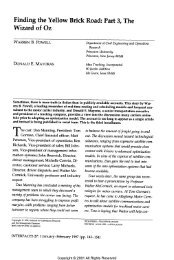
The optimal solution set is the set argmin Cf = {x ∈ C : f(x) = minCf}. For 

ɛ > 0, the ɛ-optimal solution set is the set 

argmin C,ɛ f = {x ∈ C : f(x) ≤ minCf +ɛ}. If argmin C f is a singleton {s}, we 

write s = argmin Cf. For an illustration, see Figure 1 one the next slide. 


2 

1 

0 


x 2 

−1 

2 

0 

x 

1 

4 

1 

0 

−1 

2 

0 

x 

1 

6 

1 

0 

−1 0 1 

2 

1 

0 

x 2 − 0.5x 

−1 0 1 

2 

1 

0 

x 4 − 0.5x 

−1 0 1 

2 

1 

0 

x 6 − 0.5x 

−1 0 1 

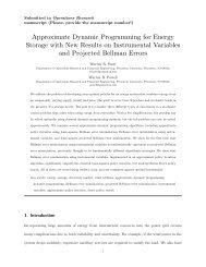
Figure: Minimizing x 2m over the domain C = [0,1], for m = 1,2,3. If the objective is 

perturbed by −0.5x (tilt perturbation), the optimal solution is less “stable” with 

higher values of m. The ɛ-optimal solution sets are shown for ɛ = 0.05. 


Questions 


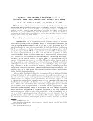
Suppose that we have an objective function fθ and a set Cθ that depend on 

some parameter θ ∈ Θ (See Figure 2 on the next slide). We would ask questions 

including: 

• What are conditions on Θ ensuring that minCθ fθ is finite for all θ ∈ Θ? 

• Given Θ, what is the range of the optimal value mapping θ ↦→ minCθ fθ? 


θ = [ −0.06 1.64 2.13 −0.70 ] 

4 

T 

3 

2 

1 

0 

−2 0 2 

3 

2 

1 


θ = [ −0.26 1.44 1.93 −0.90 ] 

4 

T 

0 

−2 0 2 

Cθ = {x ∈ R2 ⎢ 

: Ax θ} where A = ⎢ 

⎣ 

⎡ 

θ = [ −0.46 1.24 1.73 −1.10 ] 

4 

T 

3 

2 

1 

−0.83 −0.43 

0.57 0.63 

0.28 0.80 

1.14 −0.90 

0 

−2 0 2 

⎤ 

⎥ 

⎦ 

⎡ 

⎢ 

and θ = ⎢ 

⎣ 

θ = [ −0.66 1.04 1.53 −1.30 ] 

4 

T 

3 

2 

1 

0 

−2 0 2 

−0.06 

1.64 

2.13 

0.70 

⎤ 

⎡ 

⎥ 

⎦−0.2k ⎢ 

⎣ 

Figure: Convex polyhedra described by Cθ k = {x ∈ R 2 : Ax θk}, for k = 0,1,2,3 

(left to right). 

Boris Defourny (ORFE) Lecture 6: Perturbation Analysis in Optimization March 15,2012 6 / 26 

1 

1 

1 

1 

⎤ 

⎥ 

⎦

Hölder and Lipschitz Continuity for Functions 








Definition 1 (distance from a point to a set) 

The distance from a point x ∈ X to a set S ⊂ X is written 

dist(x,S) = infs∈S x −s. 

Definition 2 (neighborhood of a set) 

A neighborhood of a set S ⊂ X, written NS, is a set that is a neighborhood of 

each point of S. 



Definition 3 (Hölder condition of degree α) 

A function f(x) satisfies the Hölder condition of degree α on a set S ⊂ X (for 

some α ≥ 0) if there exists a constant c ≥ 0 such that 

|f(x)−f(y)| ≤ cx −y α for all x,y ∈ S. (1) 

When α = 1, it corresponds to Lipschitz condition. 

Definition 4 (modulus) 

The smallest possible constant c > 0 satisfies Hölder condition of function f(x) 

and the degree α. Note here we implicitly assume f(x) is of real value. A 

similar definition could be easily obtained for vector-valued function where 

|f(x)−f(y)| is replaced by f(x)−f(y). 


Example 1 


f0(x) = ax α with α ∈ (0,1] and α ∈ R satisfies |f0(x)−f0(y)| ≤ |a||x −y| α on 

C = [0,u]. 

Example 2 

Let f be a continuous function differentiable on an open set S, with gradient 

∇f(x) on S. Let C be a compact convex subset of S. Then f is Lipschitz 

continuous on C modulus c = maxx∈C∇xf(x). 



Growth Conditions 






Motivation 


This section presents notions for ensuring that a function of interest is not ”too 

flat”. Objective functions that are too flat in a neighborhood of their optimal 

solution lead to minimization problems where solutions can be very sensitive to 

perturbations. This may not be too annoying if the utility derived from the 

optimization model is well reflected by the value of objective function. However, 

there exist settings where the utility of the model is also derived from the 

solution itself. 



Definition 6(γ-order growth condition) 

Consider a function f and a nonempty set C ⊂ X. Let S ⊂ C be a nonempty 

set where f is constant-valued with value fS ∈ R: 

f(s) = fS for all s ∈ S. 

The γ-order growth condition(γ > 0) holds for f in C if there exists a constant 

c > 0 and a neighborhood NS of S such that 

f(x)−fS ≥ c[dist(x,S)] γ 

for all x ∈ NS C. 


Remark 


Ideally, we are interested in the largest c > 0 that can satisfies the inequality for 

a fixed γ. Compared to Hölder-type conditions, here only x needs to vary, and 

the absolute value is not taken on the left-hand side. Hence in practice, S 

stands for a set of local minimizers. 



Example(strongly convex function) 

Let f(x) be a twice differentiable, strongly convex function over a convex set C 

comprising its minimum: there exists a constant m > 0 such that ∇ 2 f(x) mI 

for all x ∈ C. Since for any x,y ∈ C, there exists a point z = tx +(1−t)y with 

t ∈ [0,1] such that 

f(y)−f(x) = ∇f(x) ⊤ (y −x)+ 1 

2 (y −x)⊤ ∇ 2 f(z)(y −x) , 

we have, by the strong convexity assumption, 

f(y)−f(x) ≥ ∇f(x) ⊤ (y −x)+ m 

2 ||y −x||2 . 

Consider S = argmin Cf, s ∈ S, and write fS = minC f. We have 

f(y)−fS ≥ ∇f(s) ⊤ (y −s)+ m 

2 ||y −s||2 ≥ m 

2 ||y −s||2 , 

using the fact that ∇f(s) ⊤ (y −s) ≥ 0 for all y ∈ C and s ∈ S, by optimality of 

S. This proves that S is in fact reduced to {s}, and that the second-order 

growth condition holds with modulus c = m/2: 

f(x)−fS ≥ c[x −dist(x,S)] 2 

for all x ∈ C. 



First- and Second-Order Expansions 






Directionally Differentiable 


A function g(x) is directionally differentiable at x if the directional derivatives 

exist for all directions h. 

Remark 

g ′ (x,h) = lim 

t→0 + 

g(x +th)−g(x) 

t 

If g(x) is directional differentiable, we can expand g(x +th) for t > 0 as 

g(x +th) = g(x)+tg ′ (x,h)+o(t). 


Second-Order Expansions 


A directionally differentiable function g(x) is second order directionally 

differentiable at x in the direction h if the (parabolic) second order directional 

derivatives 

g ′′ (x,h,w) = lim 

t→0 + 

g(x +th+ t2 

2w)−[g(x)+tg′ (x,h)] 

t 

exist for all (parabolic) directions w. In that case we can expand 

g(x +th+ t2 

2 w) for t > 0 as 

g(x +th+ t2 

2 w) = g(x)+tg′ (x,h)+ t2 

2 g′′ (x,h,w)+o(t 2 ). 



Perturbation Theorems 






Fixed Feasible Set 


Consider the optimization problem 

minimize f(x) 

subject to x ∈ C, 

where C ⊂ R n . Let ¯v = minCf and Sf = argmin Cf. Assume that 

• A1. Sf is nonempty. 

• A2. f satisfies a γ-order growth condition with modulus c in a 

neighborhood N of argmin C f. 


(2)

Perturbed Optimization Problem 


Consider the perturbed optimization problem 

where we assume that 

minimize f(x)+η(x) 

subject to x ∈ C, 

• B1. η is Lipschitz continuous modulus κ on C N. 

Let g(x) = f(x)+η(x), and consider any ɛ-optimal solution ˜xg ∈ argmin C,ɛg 

such that ˜xg ∈ N. 


(3)


Theorem 1 [Bonnans and Shapiro(2000)] 

Under the assumptions A1, A2 and B1, the distance between ˜xg and 

Sf = argmin Cf satisfy the relation 

c[dist(˜xg,Sf)] γ ≤ κdist(˜xg,Sf)+ɛ. 

In particular, for the second-order growth condition, the relation yields 

dist(˜xg,Sf) ≤ 1 

 

κ/c + ( 

2 1 

2 κ/c)2 +ɛ/c 

≤ κ/c + ɛ/c 

For the first-order growth condition, if κ < c, the relation yields 

dist(˜xg,Sf) ≤ ɛ/(c −κ). 


Proof of Theorem 1 


Consider ˜xf ∈ argmin Cf, and ˜xg ∈ argmin C,ɛg N. We have 

g(˜xg) ≤ minCg +ɛ ≤ g(¯xf)+ɛ, implying g(˜xg)−g(¯xf) ≤ ɛ. Therefore, 

f(˜xg)−f(¯xf) = g(˜xg)−η(˜xg)−[g(¯xf −η(¯xf)] 

= g(˜xg)−g(¯xf)+η(¯xf)−η(˜xg) ≤ ɛ+κ˜xg −¯xf, 

where the last inequality is obtained by using the Lipschitz condition on η. On 

the other hand, f(˜xg)−f(¯xf) ≥ c[dist(˜xg,Sf)] γ . For any δ > 0, we can choose 

¯xf such that ˜xg −¯xf ≤ dist(˜xg,Sf)+δ. Therefore 

f(˜xg)−f(¯xf) ≥ c[˜xg −¯xf−δ] γ . 

We have thus obtained c[˜xg −¯xf−δ] γ ≤ ɛ+κ˜xg −¯xf. By letting δ → 0 

yields ˜xg −¯xf → dist(˜xg,Sf) and the relation 

cy γ ≤ ɛ+κy 

where y = dist(˜xg,Sf) ≥ 0. The results for particular values of γ follow by 

solving for y. When γ = 2 one has to solve cy 2 −κy −ɛ ≤ 0,y ≥ 0. When 

γ = 1 one has to solve (c −κ)y ≤ ɛ,y ≥ 0. 


More Assumptions 


More can be said under additional conditions. Assume that 

• A3. The set C is compact. We define a convex compact set U ⊂ R n such 

that X ⊂ intU. 

• A4. f is Lipschitz continuous on U. 

• A5. Sf = argmin Cf is a singleton. We write ¯x = argmin Cf. 

• A2’. f satisfies a quadratic growth condition at ¯x, modulus c on U. 

• A6. f is twice continuously differentiable at ¯x. In particular we can expand 

f(x(t)) where x(t) = x +th+ t2 

2 +o(t2 ) as follows: 

f(x(t)) = f(¯x)+tf ′ (x,h)+ t2 

2 f ′′ (x,h,w)+o(t 2 ) 

= f(¯x)+t∇f(¯x) ⊤ h+ t2 

2 (∇f(¯x)⊤ w +h ⊤ ∇ 2 f(¯x)h)+o(t 2 ). 

• A7. C is convex polyhedral. 


More Assumptions... 


For t > 0, consider the perturbed problems 

P(t) : minimize f(x)+tηt(x) subject to x ∈ X, 

where the perturbations ηt(x) satisfy the following assumptions: 

• B1’. The functions ηt are Lipschitz continuous on U. 

• B2. ηt converges to a function which is Lipschitz continuous as t ↓ 0. 

• B3. The function η is differentiable at ¯x. In particular we can expand 

η(x(t)) where x(t) = x +th+ t2 

s w +o(t2 ) as follows: 

η(x(t)) = η(¯x)+t∇η(¯x)h+o(t). 

Let gt(x) = f(x)+tηt(x), and consider v(t) = minCg and ¯x(t) = argmin C gt. 



Theorem 2[Shapiro, Dentcheva, and Ruszczyński(2009)] 

Under all the assumptions we have made in the previous two slides, for t ≥ 0, 

we have the second-order expansion of the optimal function 

v(t) = ¯v +tηt(¯x)+ t2 

2 hf,η(¯x)+o(t 2 ), 

where hf,η(¯x) is the optimal value of the auxiliary problem over h, 

minimize 2h ⊤ ∇η(¯x)+h ⊤ ∇ 2 f(¯x)h 

subject to h ∈ C crit (¯x) := {d ∈ TC(¯x) : d ⊤ ∇f(¯x) = 0}, 

TC(x) := {c ∈ R n : dist(x +td,C) = o(t),t ≥ 0}. 

Moreover, if the solution to the auxiliary problem is a unique, say ¯g, we have for 

t ≥ 0 the first-order expansion of the optimal solution 

˜x(t) = ¯x +t ¯ h+o(t). 



J.F. Bonnans and A. Shapiro. 

Perturbation Analysis of Optimization Problems. 

Springer, New York, 2000. 

W. Cook, A.M.H. Gerards, and A. Schrijver. 

Sensitivity theorems in integer linear programming. 

Mathematical Programming, 34:251–264, 1986. 

O.L. Mangasarian. 

Nonlinear Programming. 

SIAM, 1994. 

R.T. Rockafellar and R.J.-B. Wets. 

Variational Analysis. 

Springer, third edition, 1998. 

A. Shapiro, D. Dentcheva, and A. Ruszczyński. 

Lectures on Stochastic Programming: Modeling and Theory. 

SIAM, 2009.

lecture. - CASTLE Lab - Princeton University

You also want an ePaper? Increase the reach of your titles

Delete template?

Save as template?