V - CERN Accelerator School
V - CERN Accelerator School
V - CERN Accelerator School

You also want an ePaper? Increase the reach of your titles
YUMPU automatically turns print PDFs into web optimized ePapers that Google loves.
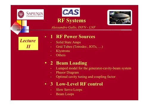
Lecture<br />
II<br />
RF Systems<br />
Alessandro Gallo, INFN - LNF<br />
1 RF Power Sources<br />
- Solid State Amps<br />
- Grid Tubes (Tetrodes , IOTs, )<br />
- Klystrons<br />
- Others<br />
2 Beam Loading<br />
- Lumped model for the generator-cavity-beam system<br />
- Phasor Diagram<br />
- Optimal cavity tuning and coupling factor<br />
3 Low-Level RF control<br />
- Slow Servo Loops<br />
- Beam Loops
RF Systems<br />
Alessandro Gallo, INFN - LNF
Various technologies available:<br />
Silicon bipolar transistors<br />
silicon LDMOS<br />
GaAsFET,<br />
Static Induction Transistors (SITs)<br />
Module<br />
schematics<br />
RF<br />
Source<br />
Solid<br />
State<br />
Frequency /<br />
Bandwidth<br />
dc 10 GHz /<br />
Large (up to<br />
multi-octave)<br />
RF Power Sources:<br />
Solid State Amplifiers<br />
Max Power<br />
0.5 kW/pallet<br />
200 kW/plant<br />
The power required is obtained by operating<br />
numerous transistors in parallel.<br />
Class of<br />
operation /<br />
Efficiency<br />
A, AB<br />
40 %<br />
Features<br />
Simplicity<br />
Modularity<br />
No HV<br />
Drawbacks<br />
Large dc currents<br />
Combiner Losses
RF Power Sources:<br />
Solid State Amplifiers<br />
352 MHz, 190 kW solid state amplifier for the SOLEIL RF System<br />
Solid State Amp. basic module<br />
Schematics of the whole power plant
RF Power Sources:<br />
Tetrodes (Grid Tubes)<br />
Tetrodes are long-time, well established grid<br />
tubes RF sources.<br />
Evolution of Triodes;<br />
Widely used in industry, TV and communications;<br />
Electrons in the tube are produced by thermo-ionic<br />
effect at the cathode;<br />
The intensity of the captured current at the Anode<br />
electrode is modulated by the Control grid<br />
potential;<br />
Screen grid increases RF isolation between<br />
electrodes.<br />
RF<br />
Source<br />
Tetrodes<br />
Frequency /<br />
Bandwidth<br />
50 1000 MHz /<br />
few %<br />
Max Power<br />
200 kW/tube<br />
Class of<br />
operation /<br />
Efficiency<br />
A, AB, B, C<br />
70 %<br />
Features<br />
Simplicity<br />
Cheap<br />
Drawbacks<br />
HV<br />
Transit-time<br />
limited
RF Power Sources:<br />
Tetrodes (Grid Tubes)<br />
Tests of the 73 MHz, 50 kW Tetrode<br />
Amplifier for the DAFNE damping ring
RF Power Sources:<br />
Inductive Output Tubes (Grid Tubes)<br />
Inductive Output Tubes (IOTs) are grid tubes<br />
(also known as klystrodes ) commercially available<br />
since 80s. They combine some design aspects of<br />
tetrodes and klystrons:<br />
Anode grounded and separated from collector;<br />
Tube beam current intensity modulated by the RF on the<br />
grid. RF input circuit is a resonant line;<br />
Short accelerating gap to reduce transit-time, beam<br />
emerging from a hole in the anode;<br />
RF output extracted from a tuned cavity between anode<br />
and collector decelerating the bunched beam;<br />
High efficiency, widely used in TV and<br />
communications.<br />
RF Source<br />
Inductive<br />
Output Tubes<br />
(IOTs)<br />
Frequency /<br />
Bandwidth<br />
100 2000 MHz<br />
/<br />
few %<br />
Max Power<br />
500 kW/tube<br />
Class of<br />
operation /<br />
Efficiency<br />
B, C<br />
80 %<br />
Features<br />
Efficient<br />
Reliable<br />
Cheap<br />
Drawbacks<br />
HV<br />
Power limited<br />
(@ high freq.)
RF Power Sources:<br />
Inductive Output Tubes (Grid Tubes)<br />
New 150 kW CW transmitter for the ELETTRA<br />
Synchrotron Light Source based on 2 80 kW IOTs
RF Power Sources:<br />
Klystrons (Velocity Modulation Tubes)<br />
The klystron has been invented in<br />
late 30s by Hansen and Varian Bros.<br />
Based on the velocity modulation concept;<br />
After being accelerated to a non-relativistic<br />
energy in an electrostatic field, a thermoionic<br />
beam is velocity-modulated crossing<br />
the gap of an RF cavity (buncher) excited by<br />
the RF input signal.<br />
Velocity modulation turns into density<br />
modulation after the beam has travelled a<br />
drift space. RF power output is extracted<br />
from a tuned output cavity (catcher) excited<br />
by the bunched beam.<br />
Other passive cavities are generally placed<br />
between buncher and catcher to enhance the<br />
bunching process.<br />
Beam particle transverse motion is focused<br />
all over the fly by solenoidal magnetic fields.<br />
Operation as oscillator is possible by feeding<br />
back an RF signal from catcher to buncher.
RF Power Sources:<br />
Klystrons (Velocity Modulation Tubes)<br />
The klystron is the most widely diffused RF source in<br />
particle accelerators. A large variety of tubes exists for different<br />
applications, spanning wide ranges of frequency and output power,<br />
as well as different duty cycles. Principal tube categories are:<br />
High power CW tubes (up to 2 MW), for synchrotron, storage rings<br />
and CW linacs;<br />
Very high peak power (up to 100 MW) tubes for low duty-cycle<br />
machines (1 4 s, 100 Hz rep rate), such as S-band, C-band (and<br />
proposed X-band) normal-conducting linacs;<br />
High peak power (up to 10 MW) tubes for high duty cycle machines<br />
(1 ms, 10 Hz rep rate), such as SC linacs for FEL radiation<br />
production or for future linear colliders. Multi-beam klystrons have<br />
been developed for this task.<br />
RF Source<br />
Klystrons<br />
Frequency /<br />
Bandwidth<br />
0.3 30 GHz /<br />
1 %<br />
Max Power<br />
2 MW rms<br />
100 MW peak<br />
Efficiency<br />
=40 60 %<br />
Collector<br />
Catcher<br />
cavity<br />
3<br />
Buncher<br />
cavity 2<br />
Insulated<br />
cathode<br />
Features<br />
High power<br />
High gain<br />
1<br />
5<br />
HV<br />
4<br />
RF<br />
output<br />
Drawbacks<br />
Efficiency
E3712 Toshiba<br />
S-band Klystron<br />
f = 2856 MHz<br />
P = 80 MW pk<br />
= 44 %<br />
Gain = 53 dB<br />
RF Power Sources:<br />
Examples of klystrons<br />
TH 2132<br />
S-band Klystron<br />
f = 2998.5 MHz<br />
P = 45 MW pk /<br />
20 kW rms<br />
= 43 %<br />
Gain = 54 dB typical<br />
NLC Klystron<br />
f = 11.4 GHz<br />
V 0 =490 kV<br />
I 0 = 260 A<br />
P = 75 MW peak<br />
= 55 %<br />
MBK<br />
for TESLA<br />
f = 1300 MHz<br />
V 0 =115 kV<br />
I 0 = 133 A<br />
P = 9.8 MW peak<br />
= 64 %<br />
Beams = 6<br />
TH 2089 Klystron<br />
for LEP<br />
f = 352 MHz<br />
P = 1.3 MW CW<br />
= 65 %<br />
Gain = 40 dB min.
RF Power Sources:<br />
Klystron Pulsed Modulators<br />
Pulsed modulators provide HV pulses to operate the klystrons in pulsed<br />
regime. To reach the highest klystron peak power the required HV can get close to 0.5<br />
MV, with pulse duration in the 1 5 s range, and acceptable pulse shape.<br />
HV pulsed modulators are then a technical and technological issue, and might in the<br />
end limit the maximum available RF power from a power plant.<br />
Thyratron switch<br />
Solid state switch
RF Power Sources (Others):<br />
Magnetrons<br />
In a Magnetron the cathode and anode have a coaxial structure, and a longitudinal<br />
static magnetic field (perpendicular to the radial DC electric field) is applied . The cylindrical<br />
anode structure contains a number of equally spaced cavity resonators and electrons are<br />
constrained by the combined effect of a radial electrostatic field and an axial magnetic field. The<br />
output power is coupled out from one of the cavities connected to a load through a waveguide.<br />
The cavity oscillations<br />
produce electric fields that<br />
spread outward into the<br />
interaction space and energy<br />
is transferred from the radial<br />
DC field to the RF field by<br />
electrons whose trajectory is<br />
bent by the magnetic field.<br />
Magnetrons have a wide<br />
range of output powers, from<br />
1 kW to 1 MW.<br />
Typical DC-to-RF powerconversion<br />
efficiency ranges<br />
from 50 to 85 %.
RF Power Sources (Others):<br />
Travelling Wave Tubes (TWTs)<br />
Helix Travelling Wave Tubes are widely used -wave amplifiers mainly consisting in:<br />
an electron gun;<br />
a focusing magnetic structure controlling the beam transverse size along the tube;<br />
an helix waveguide excited by the input RF signal whose fields interact with the electron beam,<br />
leading to the amplification process. The pitch to circumference of the helix is such that the<br />
longitudinal phase velocity of the wave equals that of the electrons;<br />
a collector to collect the electrons.<br />
The axial phase velocity is relatively constant over a wide range of frequencies, and this<br />
accounts for the large TWT bandwidths.<br />
Amplification is due to a<br />
continuous bunching of<br />
the beam allowing the<br />
energy transfer from the<br />
beam to the helix.<br />
Typical gains are 40 to<br />
60 dB while DC-to-RF<br />
conversion efficiency is<br />
in the range of 50 75 %. Helix Travelling Wave Tube Sketch
RF Power Sources:<br />
Pulse Compression (SLED)<br />
The Stanford Linac Energy Doubling (SLED) is a system developed to compress RF<br />
pulses in order to increase the peak power (and the available accelerating gradients) for a given<br />
total pulse energy. This is obtained by capturing the pulsed power reflected by a high-Q cavity<br />
properly excited by the RF generator (typically a klystron). In fact the wave reflected by an<br />
overcoupled cavity ( 5) peaks at the end of the RF pulse to about twice the incident wave level<br />
(with opposite polarity).<br />
By playing with this, and properly tailoring the incident<br />
wave, accelerating gradients integrated over a small portion<br />
of the original pulse duration almost doubled.
RF Systems<br />
Alessandro Gallo, INFN - LNF
STATIC BEAM LOADING<br />
We know from the longitudinal<br />
dynamics theory of storage rings that the<br />
motion of a single particle is stably focused<br />
around an equilibrium position known as<br />
synchronous phase .<br />
The synchronous phase corresponds to an<br />
accelerating voltage on the particle equal to its<br />
average single-turn loss, which accounts for<br />
synchrotron radiation emission and interaction<br />
with the vacuum chamber wakefields. In<br />
synchrotrons this also accounts for the<br />
required energy gain/turn during ramping.<br />
For storage rings with positive dilation factor<br />
the synchronous phase is placed on the<br />
accelerating voltage positive slope; the<br />
contrary for negative dilation factor rings.<br />
The particle absorbs energy from the accelerating field but also contributes to the total voltage.<br />
The particle induced voltage can be easily calculated treating the cavity accelerating mode as a<br />
lumped resonant RLC resonator interacting with an impulsive current.<br />
f<br />
p<br />
f<br />
p<br />
1<br />
2<br />
c
THE CAVITY RLC MODEL<br />
The beam-cavity interaction can be conveniently described by introducing the resonator<br />
RLC model. According to this model, the cavity fundamental mode interacts with the beam current<br />
just like a parallel RLC lumped resonator. The relations between the RLC model parameters and<br />
the mode field integrals r (mode angular resonant frequency), V c<br />
(maximum voltage gain for a<br />
particle travelling along the cavity gap for a given field level), U (energy stored in the mode), P d<br />
(average power dissipated on the cavity walls) and Q (mode quality factor), are given by:<br />
V<br />
U<br />
Mode field integrals<br />
c<br />
P<br />
d<br />
Q<br />
gap<br />
1<br />
2<br />
1<br />
4<br />
V<br />
E<br />
S<br />
R<br />
rU<br />
;<br />
P<br />
d<br />
(<br />
z<br />
( z)<br />
e<br />
surf<br />
E<br />
2<br />
H<br />
j<br />
2<br />
t<br />
d<br />
R / Q<br />
r<br />
H<br />
z<br />
c<br />
2<br />
dz<br />
) d<br />
V<br />
2<br />
2<br />
c<br />
r<br />
U<br />
Cavity RLC model<br />
Note:<br />
we assume that positive voltages accelerate<br />
the beam, which is therefore modelled as a<br />
current generator discharging the cavity<br />
RLC parameters<br />
R<br />
C<br />
L<br />
s<br />
r<br />
2<br />
r<br />
2<br />
c<br />
V<br />
2P<br />
1<br />
d<br />
1<br />
R<br />
C<br />
Q<br />
R<br />
Q<br />
r
v<br />
( t)<br />
V<br />
q<br />
q<br />
C<br />
V<br />
q<br />
STATIC BEAM LOADING<br />
A particle travelling along the cavity gap is a<br />
function current generator exciting the RLC resonator. The<br />
particle induced voltage in the cavity vq (t) is a decaying cosine<br />
wave generated at the particle passage. The fundamental<br />
theorem of beam loading states that the particle sees only half<br />
of its induced voltage step Vq . According to the model, the<br />
expression for vq (t) is:<br />
q<br />
q<br />
1(<br />
t<br />
r<br />
R<br />
t<br />
q<br />
Q<br />
)<br />
cos<br />
The particle in a storage ring are gathered in bunches that<br />
typically show a gaussian longitudinal profile. The bunches are<br />
normally much shorter than the RF wavelength and interact<br />
with the accelerating field similarly to macroparticles. The<br />
voltage induced in the cavity by a short gaussian bunch is still<br />
an exponentially decaying cosine wave with a finite rise time<br />
(related to the bunch duration).<br />
r<br />
( t<br />
t<br />
q<br />
)<br />
e<br />
r<br />
( t<br />
2Q<br />
t<br />
q<br />
)
STATIC BEAM LOADING<br />
It can be easily verified that both<br />
the amplitude and the slope of the voltage<br />
induced in a cavity by a single passage of<br />
a short bunch are almost negligible with<br />
respect to the cavity accelerating voltage.<br />
What can not in general be neglected is<br />
the voltage generated by the cumulative<br />
effect of many bunch passages.<br />
N<br />
In fact, the time distance between adjacent bunches T b<br />
is normally much smaller than the cavity filling time f.<br />
This is true even in single bunch operation whenever<br />
the ring revolution period is smaller than the cavity<br />
filling time. In this case the voltage kicks associated to<br />
the passage of the bunches add coherently, and the<br />
overall beam induced voltage can grow substantially<br />
and even exceed the generator induced voltage.<br />
T<br />
f<br />
b
STATIC BEAM LOADING<br />
The cumulative contribution of many bunch passages depends essentially on the RF<br />
harmonic of the beam spectrum. Also neighbour lines play a role in case of uneven bunch filling<br />
pattern (gap transient effect).<br />
The static beam loading problem consists in computing:<br />
- the overall contribution of the beam to the accelerating voltage;<br />
- the power needed from the RF generator to refurnish both<br />
cavity and beam;<br />
- the optimal values of cavity detuning and cavity-to-generator<br />
coupling to minimize the power request to the generator.<br />
P<br />
FWD<br />
n<br />
R<br />
s<br />
2<br />
Z0<br />
V<br />
2<br />
FWD<br />
2Z<br />
0
Y<br />
L<br />
I<br />
V<br />
I<br />
T<br />
c<br />
g<br />
1<br />
R<br />
2V<br />
n Z<br />
STATIC BEAM LOADING<br />
To solve the static beam loading problem we refer to the following circuital model:<br />
L<br />
FWD<br />
0<br />
j<br />
2q<br />
I b ;<br />
T<br />
b<br />
C<br />
8<br />
P<br />
R<br />
b<br />
s<br />
1<br />
L<br />
FWD<br />
s<br />
The beam current is represented by the phasor Ib at the frequency of the RF source, while the<br />
external RF source is represented by a current generator Ig whose amplitude is related to the<br />
power of the forward wave launched on the transmission line.<br />
If > 0 the beam current phasor anticipates the total cavity voltage (i.e. s > 0), while it is<br />
retarded in the opposite case ( < 0 s < 0 ).<br />
The RF sources are normally specified by the maximum amount of power deliverable on a<br />
matched load. This is also the power actually dissipated in the system whenever a circulator is<br />
interposed to protect and match the source. The cavity is usually tuned near the optimal value<br />
that minimizes the request of forward RF power to the generator.
The analysis of the beam-cavity circuital<br />
model leads to the reported phasor diagram. The total<br />
current exciting the cavity is:<br />
I<br />
T<br />
I<br />
g<br />
I<br />
b<br />
V<br />
c<br />
Y<br />
V<br />
c<br />
Real and imaginary parts of the generator current are<br />
then given by:<br />
Re<br />
I<br />
Im I<br />
g<br />
g<br />
Re I<br />
Im I<br />
T<br />
T<br />
I<br />
I<br />
b<br />
b<br />
V<br />
V<br />
c<br />
c<br />
R<br />
s<br />
R<br />
1<br />
r<br />
s<br />
R<br />
1<br />
I<br />
Q<br />
b<br />
r<br />
j<br />
cos<br />
C<br />
s<br />
I<br />
b<br />
1<br />
L<br />
sin<br />
s<br />
the minimum generator current amplitude, corresponding to the optimal cavity tuning, is obtained<br />
when its imaginary part is zero:<br />
Im I<br />
g<br />
0<br />
V<br />
c<br />
R<br />
STATIC BEAM LOADING<br />
Being the off-resonance parameter defined as:<br />
Q<br />
I<br />
b<br />
sin<br />
s<br />
I<br />
b<br />
c<br />
r<br />
R Q<br />
sin<br />
V<br />
s<br />
r<br />
2<br />
g<br />
z<br />
sgn<br />
s<br />
0<br />
0<br />
r<br />
2q<br />
T<br />
0<br />
b<br />
0<br />
b<br />
R Q<br />
V<br />
c<br />
1<br />
s<br />
V<br />
V<br />
0<br />
g<br />
c<br />
z<br />
loss<br />
0<br />
2<br />
0<br />
0
I<br />
g<br />
STATIC BEAM LOADING<br />
The optimal cavity tuning condition in<br />
a storage ring with negative dilation factor asks<br />
for positive values of . This means that the cavity<br />
has to be tuned below the frequency of the RF<br />
generator, and the amount of detuning is<br />
proportional to the intensity of the stored current.<br />
The sign of the detuning is just opposite for<br />
positive values of the dilation factor<br />
Under the optimal cavity tuning condition we also<br />
have:<br />
1<br />
8 PFWD<br />
Rs<br />
1<br />
Re I g Vc<br />
Ib<br />
cos s<br />
PFWD<br />
Vc<br />
Ib<br />
cos s<br />
R<br />
R<br />
8 R<br />
leading to the optimal coupling condition:<br />
s<br />
It follows immediately that the forward power<br />
request to the external generator is:<br />
s<br />
opt<br />
I<br />
R<br />
b s<br />
b s loss<br />
1 cos s 1 2<br />
Vc<br />
Vc<br />
1 c 1<br />
PFWD Ib<br />
Vc<br />
cos<br />
2 Rs<br />
2<br />
2<br />
The system is perfectly matched and no RF power is wasted because of reflections.<br />
I<br />
0<br />
Vc<br />
1<br />
R sin<br />
V<br />
s<br />
< 0 > 0<br />
s<br />
I<br />
s<br />
R<br />
V<br />
s<br />
P<br />
1<br />
cav<br />
P<br />
P<br />
cav<br />
2<br />
beam<br />
P<br />
beam
The beam can be also<br />
modelled as a complex<br />
admittance equal to the ratio<br />
between the current and voltage<br />
phasors. This model is less<br />
physical (the resistive part of the<br />
beam admittance does not<br />
enlarge the bandwidth of the<br />
cavity!) but allows more direct<br />
computation of the reflection<br />
coefficient at the coupling port.<br />
R<br />
Z<br />
STATIC BEAM LOADING<br />
s Ycav<br />
0<br />
R<br />
Z<br />
Y<br />
cav<br />
s Ybeam<br />
0<br />
1<br />
R<br />
s<br />
j<br />
R<br />
1<br />
1<br />
Q<br />
Rs 2<br />
n Z<br />
Zero for optimal<br />
coupling factor<br />
Rs<br />
I<br />
V<br />
c<br />
Rs<br />
I<br />
V<br />
c<br />
0<br />
Ib<br />
j Ib<br />
I<br />
Y b<br />
beam e s cos s j sin<br />
V V V<br />
b<br />
b<br />
cos<br />
cos<br />
c<br />
s<br />
s<br />
jR<br />
jR<br />
s<br />
s<br />
c<br />
Zero for optimal<br />
cavity detuning<br />
R<br />
R<br />
Q<br />
Q<br />
I<br />
V<br />
b<br />
c<br />
I<br />
V<br />
b<br />
c<br />
c<br />
sin<br />
sin<br />
Ybeam<br />
s<br />
s<br />
s
STATIC BEAM LOADING<br />
For a given required cavity voltage V c , the optimal values of the cavity detuning<br />
and coupling coefficient are both dependent on the instantaneous stored current I b . The<br />
accelerating cavities are equipped with tuners, that are devices allowing small and continuous<br />
cavity profile deformation to real time control the resonant frequency position.<br />
Sometimes cavities are also equipped with<br />
variable input couplers but they are never operated<br />
in regime of continuous adjustment. In general<br />
the coupling coefficient is adjusted just once to<br />
match the maximum expected beam current. At<br />
lower currents the system is partially mismatched,<br />
but the available RF power is nevertheless<br />
sufficient to feed the cavity and the beam.<br />
It turns out that the cavity tuning and the<br />
generator power P FWD have to follow the actual<br />
current value in order to keep the accelerating<br />
voltage constant preserving good matching<br />
conditions. b bmax<br />
I I<br />
These tasks are normally accomplished by dedicated slow feedback systems, namely the tuning<br />
loop and the amplitude loop .
RF Systems<br />
Alessandro Gallo, INFN - LNF
TUNING LOOP<br />
The tuning loop restores automatically<br />
and continuously the cavity resonant frequency to<br />
compensate the beam reactive admittance. The<br />
loop controls the RF phase between the cavity<br />
voltage and the forward wave from the generator.<br />
Phase drifts are corrected by producing<br />
mechanical deformations of the cavity profile by<br />
means of dedicated devices (plungers, squeezers,<br />
...). In fact the loop controls the phase of the<br />
transfer function:<br />
1<br />
2<br />
Vc<br />
n Ycav<br />
Ybeam<br />
2n<br />
V<br />
1<br />
FWD Z 0 2<br />
n Y Y<br />
V<br />
V<br />
c<br />
FWD<br />
Q<br />
R<br />
cav<br />
L b<br />
arctan<br />
L<br />
1<br />
Vc<br />
RLI<br />
b cos<br />
Vc<br />
s<br />
s<br />
with<br />
I<br />
sin<br />
beam<br />
Q<br />
R<br />
L<br />
L<br />
1<br />
Q<br />
1<br />
R<br />
1<br />
0<br />
s<br />
R<br />
s<br />
Beam<br />
Y<br />
2n<br />
cav<br />
Y<br />
beam<br />
1<br />
1<br />
jQ<br />
2<br />
L<br />
R<br />
Z 0<br />
RLI<br />
V<br />
By controlling the set point of the<br />
variable phase shifter the phase of<br />
the transfer function can be locked<br />
to 0 or to any other value 0 .<br />
c<br />
s<br />
b<br />
e<br />
j<br />
s
TUNING LOOP<br />
The best cavity tuning is obtained by locking the loop to 0 = 0. In this case we have:<br />
RLI<br />
b QL<br />
sin s<br />
Vc<br />
RLI<br />
b<br />
Ib<br />
R Q<br />
arctan 0 QL<br />
sin s 0<br />
sin s 0<br />
RLI<br />
b<br />
V<br />
1 cos<br />
c<br />
Vc<br />
s<br />
Vc<br />
For dynamics considerations, sometimes it is useful to set a phase 0 slightly different from zero.<br />
In this case we have: RLI<br />
b QL<br />
sin s<br />
Vc<br />
RLI<br />
b<br />
RLI<br />
b<br />
arctan 0 QL<br />
sin s tan 0 1 cos s<br />
RLI<br />
b<br />
Vc<br />
V<br />
1 cos<br />
c<br />
s<br />
V<br />
0<br />
1<br />
j tan<br />
j tan<br />
0<br />
0<br />
c<br />
with<br />
0<br />
1<br />
1<br />
1<br />
RLI<br />
V<br />
RL<br />
I<br />
V<br />
c<br />
b<br />
c<br />
b<br />
cos<br />
cos<br />
s<br />
s<br />
The reflection at the input<br />
coupler port is not<br />
minimized in this case,<br />
and the overall efficiency<br />
of the system is reduced.<br />
Tuning loops are generally very slow since they involve mechanical movimentation through the<br />
action of motors. Typical bandwidth of such systems are of the order of 1 Hz. Tuning systems<br />
are also necessary to stabilize the cavity resonance against thermal drifts.
AMPLITUDE LOOP<br />
The automatic regulation of the generator<br />
output level can be obtained by implementing<br />
amplitude loops. These are feedback systems<br />
which detect and correct variations of the level of<br />
the cavity voltage.<br />
If the power amplifier is not fully saturated, the<br />
regulation can be obtained by controlling the RF<br />
level of the amplifier driving signal.<br />
If the amplifier is saturated, the feedback has to act<br />
directly on the high voltage that sets the level of<br />
the saturated output power.<br />
Referring to the reported model, the loop transfer<br />
function can be written in the form:<br />
Ac in<br />
A<br />
ref<br />
H ( s)<br />
1 H ( s)<br />
with<br />
H ( s)<br />
A<br />
V<br />
mod<br />
K C(<br />
s)<br />
G(<br />
s)<br />
For little cavity detuning (Q L
AMPLITUDE LOOP<br />
In heavy beam loading regime the cavity<br />
detuning is likely to be as large as the cavity bandwidth<br />
or even more, so that the single pole model for the<br />
cavity amplitude response is inappropriate. A more<br />
complex model applies in this case, involving crossmodulation<br />
blocks.<br />
Amplitude loops may have bandwidths ranging from<br />
few Hz to 1 MHz. Sometimes it is useful to have large<br />
residual loop gain at line frequencies to correct spurious<br />
modulation introduced by the power stages. The gain<br />
and bandwidth can be tailored by properly designing the<br />
error amplifier transfer function G(s). For instance, if<br />
the cavity single-pole model is adequate, high loop<br />
gains in the low frequency region are obtainable by<br />
implementing an integrator providing a zero for<br />
compensating the cavity pole.<br />
G(<br />
s)<br />
H ( s)<br />
1 sCR2<br />
1<br />
with CR2<br />
sCR1<br />
Ain<br />
Ain<br />
KC0<br />
K C(<br />
s)<br />
G(<br />
s)<br />
Vmod<br />
Vmod<br />
sCR<br />
The low frequency gain can be boosted by properly treating the error signal. However, the<br />
coupling between the various RF servo loops induced by the large cavity detuning may result in a<br />
global instability of the beam-cavity system. To avoid it, gain and bandwidth of individual loops<br />
have to be reduced.<br />
1
The cavity RF phase (or the<br />
power station RF phase) can be locked<br />
to the reference RF clock by another<br />
dedicated servo loop. The need for a<br />
phase loop is not strictly related to beam<br />
loading effects but more to ensure<br />
synchronization between different RF<br />
cavi-ties or between RF voltage and<br />
other sub-systems of the accelerator<br />
(such as injection system, beam<br />
feedback systems, ...).<br />
PHASE LOOP<br />
Beam<br />
The phase is locked to the reference by measuring<br />
the relative phase deviation by means of a phase<br />
detector and applying a continuous correction<br />
through a phase shifter. For loop gain and bandwidth<br />
the same considerations expressed in the amplitude<br />
loop case hold.<br />
C(<br />
s)<br />
H ( s)<br />
c in<br />
ref<br />
1 H ( s)<br />
1 H ( s)<br />
c<br />
in<br />
with<br />
if<br />
H ( s)<br />
kmodkdet<br />
C(<br />
s)<br />
G(<br />
s)<br />
H ( s)<br />
C(<br />
s)<br />
; H ( s)<br />
1
The beam phase<br />
loops are feedback systems<br />
aimed at adding a damping<br />
( frictional) term in the<br />
synchrotron equation for the<br />
beam center-of-mass coherent<br />
motion.<br />
In the basic scheme the phase<br />
of the beam is detected and,<br />
after a manipulation to<br />
introduce a 90° phase shift at<br />
the synchrotron frequency, is<br />
applied back to the cavity.<br />
;<br />
Beam Phase Loop<br />
Ideally, if the cavity modulation were exactly proportional to the time derivative of the beam<br />
phase we would get:<br />
c<br />
k<br />
b<br />
b<br />
making a frictional term appearing in the synchrotron equation.<br />
2<br />
s<br />
b<br />
2<br />
s<br />
c<br />
b<br />
2<br />
s<br />
k<br />
b<br />
2<br />
s<br />
b<br />
0
An Example: PEP-II<br />
Low Level RF Control Loops