3D EM Simulations
3D EM Simulations
3D EM Simulations

You also want an ePaper? Increase the reach of your titles
YUMPU automatically turns print PDFs into web optimized ePapers that Google loves.
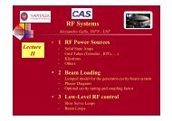
<strong>3D</strong> <strong>EM</strong> <strong>Simulations</strong><br />
1 ube / v2.0 / 2008<br />
www.cst.com
• CCavities iti<br />
– Eigenmodes<br />
–Q Factor<br />
Overview<br />
– Time Domain and Resonances<br />
• Cavities and Particles<br />
• Electron Guns<br />
• Collector<br />
• Wakefields<br />
2 www.cst.com
f<br />
Eigenmode Solver<br />
Theoretical Background<br />
PEC<br />
f f<br />
f=c/L f=c/L<br />
f=2c/L f=2c/L<br />
PMC<br />
In free space travelling waves can<br />
exist i t ffor any frequencies.<br />
f i<br />
If such a plane wave is reflected at a<br />
perfect f wall ll ( (electric l i or magnetic) i )<br />
there will be a standing wave. This<br />
standing wave exists independently<br />
from the frequency.<br />
The insertion of a second wall does<br />
not affect those standing wave as<br />
long g as the distance L between the<br />
walls fits perfectly to the wave-length.<br />
The standing wave of this closed<br />
structure is called an eigenmode.<br />
The frequency and the shape of the<br />
next eigenmode fitting between those<br />
two walls is predictable.<br />
3 www.cst.com
Eigenmode g Computation<br />
r r<br />
rot E r r=<br />
− jωμ<br />
r rH<br />
r σσ<br />
r<br />
rot H = jωε<br />
E + σ E = jω(<br />
ε + ) E =<br />
jω<br />
rot<br />
1<br />
μμ<br />
rot<br />
r<br />
E<br />
=<br />
ω<br />
2<br />
ε<br />
r<br />
E<br />
Eigenvalue equation for the resonant structure modes<br />
and resonance frequencies. q<br />
Eigenvalues ω and eigenvectors E r<br />
4 www.cst.com<br />
j<br />
ω ε<br />
r<br />
E
Eigenmodes g<br />
f1=34.7 GHz f2=52.0 GHz<br />
f3=54.3 GHz f4=57.9 GHz f5=67.7 GHz<br />
5 www.cst.com
1<br />
2<br />
Eigenmode g Solver<br />
Main user input:<br />
1<br />
2<br />
Which eigenmode method should be used?<br />
(AKS might be faster for well behaved examples,<br />
JD is more robust and might even find good<br />
solutions for bad conditioned problems)<br />
How many modes are required?<br />
The AKS method always calculates internally at<br />
least 10 modes. (Therefore ( nearly y no difference in<br />
cpu time between 1 and 10 modes).<br />
The JD method calculates one mode after<br />
another, therefore 10 modes need roughly<br />
10times the simulation time of 1 mode.<br />
Therefore the number of modes should be<br />
decreased when using the JD method.<br />
Th<br />
6 www.cst.com
A simple lossfree Cavity<br />
3 symmetry y y pplanes only y 1/8<br />
of the volume needs to be calculated<br />
Mode1<br />
E H<br />
Mode2<br />
Mode3<br />
7 www.cst.com<br />
cavity_03.zip
electric energy density<br />
0.5 ε E_peak^2<br />
Energy gy Densities<br />
magnetic energy density<br />
0.5 μ H_peak^2<br />
Volume Integration of Energy Density is possible via Result Template<br />
0D / Evaluate Field in arbitrary Coordinates (0D, 1D, 2D, <strong>3D</strong>)<br />
Note: for a lossfree eigenmode both integrals (el. + mag.energy) will be 1 Joule,<br />
since i th the energy iis oscillating ill ti bbetween t electric l t i and d magnetic ti fi field.<br />
ld<br />
8 www.cst.com
Plotting Fields and getting Field Values<br />
All modes are normed<br />
to 1 Joule stored energy.<br />
E / H / surface current<br />
are stored as peak values.<br />
9 www.cst.com
Benchmark Pillbox<br />
h1 r11 Influence of Meshing<br />
E H<br />
surface current J<br />
QQ_theory=50 theory=50 940<br />
Q_simul=50 990<br />
cpu-time<br />
pass 1 = 16sec<br />
pass 5 = 2 min<br />
f_theory=229.485MHz<br />
f_simul=229.444MHz<br />
10 pillbox_01.zip<br />
www.cst.com
The Quality y Factor Q<br />
2π<br />
• StoredEnergy<br />
2π<br />
⋅ f ⋅W<br />
Q =<br />
=<br />
Energy _ consumed _ per _ period<br />
the higher Q, the longer the energy is kept<br />
• for a lossfree structure P=0 infinite Q<br />
• different kind of losses exist:<br />
• skin effect (surface) losses: Qwall • dielectric (volume) losses: Q diel<br />
• losses due to connected feeding lines: Qext • losses due to energy transfer between beam and mode: Qbeam 1<br />
Q<br />
tot<br />
1<br />
=<br />
Q<br />
As a circuit model, all losses can be seen as a<br />
parallel circuit, acting on the same mode.<br />
wall<br />
Prms<br />
1<br />
+<br />
Q<br />
diel<br />
1<br />
+<br />
Q<br />
ext<br />
1<br />
+<br />
Q<br />
11 www.cst.com<br />
beam
Calculation of Q and Q wall diel<br />
Results -> Loss and Q-Calculation performs p a loss calculation in the<br />
postprocessing based on perturbation theory. It handles metallic losses<br />
due to finite conductivity (skin effect) as well as dielectric losses.<br />
Q=2*Pi*frq * Energy / Loss_rms<br />
frq = 2.96289815e+010 Hz<br />
Loss Loss_rms rms = 00.5 5 Loss Loss_peak peak<br />
Energy = 1 Joule<br />
12 www.cst.com
Integration of Voltage,<br />
Calculation of Shunt Impedance & R/Q<br />
Shunt Impedance Rs=Vo^2/(2W)<br />
with Vo : voltage „seen“ by a charged<br />
interacting particle.<br />
For voltage integration also the Transit Time Factor<br />
can be specified, which defines the speed of<br />
the particle (beta=v/c) ( ) and gguarantees<br />
a<br />
phase-correct integration of electr. field.<br />
R/Q (R over Q) only depends on the geometry<br />
(not on the loss mechanism) and is therefore<br />
often used to compare different cavity structures.<br />
13 www.cst.com
Example Superconducting Cavity<br />
easy construction via Macros -><br />
Construct -> Superconducting p g Cavity y<br />
ellipt_cav_01.zip<br />
14 www.cst.com
Eigenmode Solver<br />
Calc Calculation lation of Q Qext Langer filter<br />
Results of the Q-Factor calculation: Log File<br />
EE.g. g external QQ-factor factor comparison for the Langer filter<br />
f [GHz]<br />
4.546<br />
4.572<br />
7.080<br />
77.185 185<br />
CST Q_ext<br />
332<br />
305<br />
26200<br />
9070<br />
Steiglitz-McBride<br />
332<br />
305<br />
24132<br />
8472<br />
15 www.cst.com • Oct-09
Other methods for loaded Q<br />
calc calculation lation<br />
• Using the transient analysis<br />
• Amplitude E-field inside a resonator is given:<br />
) t ( E<br />
=<br />
E<br />
0 t<br />
2 Q<br />
0 e<br />
ω ⋅<br />
−<br />
⋅<br />
⋅<br />
load<br />
or<br />
ω0⋅t<br />
E( t)<br />
−<br />
2⋅Q<br />
• MMonitored it d using i an EE-field fi ld probe b<br />
• Measure the time difference Δt in which the E-field is<br />
damped by a factor of 1/e then Q load is given by<br />
load<br />
E<br />
Q = π⋅<br />
Δt<br />
⋅f<br />
16 CST Microwave Studio • www.cst-world.com • Oct-09<br />
0<br />
0<br />
=<br />
e<br />
load
Other methods for loaded Q<br />
calc calculation lation<br />
lloadd = π π⋅<br />
Δ t f 0<br />
Signal: 503.7 at t1=200 ns<br />
Signal: 503 503.7/e 7/e = at t2 t2= 423 423.6ns 6ns<br />
Δt = t2 –t1 = 223.6ns<br />
f0 = 2.4615 GHz<br />
Qload = 1729<br />
Q Δ ⋅<br />
1/e<br />
17 CST Microwave Studio • www.cst-world.com • Oct-09
Time Domain Simulation and<br />
Resonant SStructures<br />
Slow energy decay since energy is kept in the resonance<br />
Long Simulation Time<br />
Prediction of signal by Autoregressive Filter<br />
Usage of Frequency Domain Solver<br />
Transient Activity<br />
Energy Decay<br />
18 www.cst.com | Oct-09
Time Domain Simulation<br />
AR Filter<br />
Stop at 31.0 ns<br />
Without online-AR cpu=100 sec<br />
Stop at 1.4 ns<br />
With online-AR-Filter cpu=15 sec (1port)<br />
Original SS-Parameter Parameter<br />
from Time Signals<br />
S-Parameter<br />
predicted by<br />
AR Filter<br />
19 www.cst.com | Oct-09
Frequency q y Domain Solver<br />
• Simulation performed at single frequencies<br />
• Simulation of Steady State<br />
• Broadband Frequency Sweep<br />
20 www.cst.com • Oct-09
Thermal Calculation<br />
Surface and volume losses<br />
from previous eigenmode<br />
simulation can be used to perform<br />
a thermal analysis<br />
21 www.cst.com
• CCavities iti<br />
– Eigenmodes<br />
–Q Factor<br />
Overview<br />
– Time Domain and Resonances<br />
• Cavities and Particles<br />
• Electron Guns<br />
• Collector<br />
• Wakefields<br />
22 www.cst.com
Workflow:<br />
Tracking Algorithm<br />
1. Calculate electro- and magnetostatic fields<br />
2. Calculate force on charged particles<br />
3. Move particles according to the previously calculated<br />
force Trajectory<br />
d<br />
dt<br />
r<br />
r<br />
r<br />
r<br />
( m v ) )<br />
= q(<br />
E + v × B<br />
Velocity<br />
( )<br />
n+<br />
1 n+<br />
1 n n<br />
n+<br />
1/<br />
2 n+<br />
1 n+<br />
1/<br />
2<br />
= q(<br />
E + v × B<br />
y<br />
update<br />
+ Δt(<br />
E + × B )<br />
n+<br />
1 n+<br />
1 n n<br />
n+<br />
1/<br />
2 n+<br />
1 n+<br />
1/<br />
2<br />
m v = m v + qΔt<br />
E + v × B<br />
dr<br />
v<br />
ddt<br />
Position update<br />
t = n+ 3/2 n+ 1/2 n+<br />
1<br />
r<br />
r<br />
r r r<br />
r = r +Δtv<br />
23 www.cst.com | Oct-09<br />
r
Tesla-Type 9-Cell Cavity<br />
Electric Field<br />
calculated by<br />
MWS-E<br />
24 www.cst.com | Oct-09
Tesla-Type 9-Cell Cavity<br />
Particle Trajectory<br />
(color indicates the<br />
energy of the particles)<br />
25 www.cst.com | Oct-09
TESLA – Two-Point-Multipacting<br />
• Eigenmode at 1.3 GHz<br />
•Emax = 45 MV/m<br />
26 www.cst.com | Oct-09
time<br />
TESLA – Two-Point-Multipacting<br />
half hf period<br />
27 www.cst.com | Oct-09
• CCavities iti<br />
– Eigenmodes<br />
–Q Factor<br />
Overview<br />
– Time Domain and Resonances<br />
• Cavities and Particles<br />
• Electron Guns<br />
• Collector<br />
• Wakfields<br />
28 www.cst.com
Emission Models<br />
Space Charge Limited Emission:<br />
Assumption:<br />
Φ (d d d<br />
)<br />
•Unlimited number of particles<br />
•Particle extraction depends on<br />
field close to emitting surface<br />
Childs Law:<br />
J<br />
s<br />
( ) 3/2<br />
Φ( d)<br />
−Φ(0)<br />
4 q<br />
ε 2<br />
9 m d<br />
= rent<br />
2<br />
Curr<br />
PEC<br />
( 0)<br />
Φ<br />
Voltage<br />
Child-Langmuir Model<br />
d<br />
Virtual Cathode<br />
29 www.cst.com | Oct-09
Thermionic Emission:<br />
Assumption:<br />
•Limited number of particles<br />
Emission Models<br />
•Particle extraction depends on<br />
field close to emitting surface<br />
until ntil all particles are emitted<br />
Richardson Richardson-Dushman Dushman Equation:<br />
J = AT<br />
s<br />
2<br />
e<br />
eΦ<br />
-<br />
kT<br />
Currrent<br />
Temperature Limited<br />
Space Charge<br />
Limited<br />
Voltage<br />
30 www.cst.com | Oct-09
Gridded Gun<br />
control grid<br />
permanent magnets<br />
31 www.cst.com | Oct-09<br />
Potential<br />
B-Field
Gridded Gun - Mesh<br />
32 www.cst.com
33<br />
S-DALINAC Electron Source<br />
-100kV<br />
Photocathode<br />
Diagnosis and<br />
Manipulation<br />
Vacuum<br />
See also Bastian Steiner, PhD Thesis, T<strong>EM</strong>F, TU Darmstadt<br />
0V
S-DALINAC Electron Source<br />
Electron trajectory<br />
34 See also Bastian Steiner, PhD Thesis, T<strong>EM</strong>F, TU Darmstadt
S-DALINAC Electron Source<br />
Electric potential<br />
35 See also Bastian Steiner, PhD Thesis, T<strong>EM</strong>F, TU Darmstadt
• CCavities iti<br />
– Eigenmodes<br />
–Q Factor<br />
Overview<br />
– Time Domain and Resonances<br />
• Cavities and Particles<br />
• Electron Guns<br />
• Collector<br />
• Wakefields<br />
36 www.cst.com
Collector<br />
Potential<br />
37 www.cst.com | Oct-09
Collector, including secondary electron<br />
emission<br />
E0 = 50 keV E0 = 125 keV<br />
E0 = 200 keV E0 = 275 keV<br />
38 www.cst.com | Oct-09<br />
E0 = initial energy of the electrons
• CCavities iti<br />
– Eigenmodes<br />
–Q Factor<br />
Overview<br />
– Time Domain and Resonances<br />
• Cavities and Particles<br />
• Electron Guns<br />
• Collector<br />
• Wakefields<br />
40 www.cst.com
Wakefields<br />
What does the Wakefield Solver do?<br />
simple explanation: SSpecial current excitation of f CST CS MWS S T-Solver. S<br />
more complex explanation:<br />
- Moving charged particles are represented as Gaussian current density<br />
- At structure discontinuities the intrinsic electromagnetic fields of the moving<br />
charged c a ged pa particles t c es causes tthe e appea appearance a ce o of „ „Wakefields“ a e e ds<br />
- These Wakefields can act back on the particles which is expressed in terms<br />
of a Wakepotential<br />
41 www.cst.com | Oct-09
Beam Position Monitor<br />
Wakefields<br />
Note: Beta smaller<br />
than 1 is possible.<br />
detailed deta ed<br />
view<br />
42 www.cst.com | Oct-09
Beam Position Monitor<br />
150<br />
0<br />
Wakefields<br />
Port 1<br />
Port 2<br />
-150 0 7<br />
Time/ns<br />
Output Signals at the electrode<br />
ports excited by the beam<br />
Electric field vs. time<br />
43 www.cst.com | Oct-09
Wakefields<br />
Normalized<br />
output at the<br />
electrode<br />
See also: P. Raabe, VDI Fortschrittsberichte, Reihe 21, Nr. 128, 1993<br />
44 www.cst.com | Oct-09
Pillbox Cavity<br />
Structure<br />
Wakefields<br />
Beam definition<br />
45 www.cst.com | Oct-09
Wl(s)/ /(V/C)<br />
Wakefields<br />
RReference f PPulse l<br />
Wl(s)<br />
46 www.cst.com | Oct-09
Wakefields<br />
47 www.cst.com | Oct-09
Wakefields<br />
48 www.cst.com | Oct-09
• CCavities iti<br />
– Eigenmodes<br />
–Q Factor<br />
SUMMARY<br />
– Time Domain and Resonances<br />
• Cavities and Particles<br />
• Electron Guns<br />
• Collector<br />
• Wakefields<br />
49 www.cst.com