Cavity Basics - CERN Accelerator School

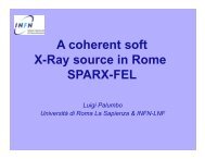
cern.ch/rf‐lectures 

SUPERFISH EXERCISE 

14‐16/6/2010 CAS RF Denmark ‐ Superfish Exercise 1

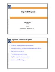
Would you 

like to design a cavity? 

• Superfish is 2‐D. The 2 coordinates can be R‐Z in cylindrical or X‐Y in cartesian. 

• Losses must be small (perturbation method). 

• Please come up with your own ideas of what you would like to do! 

• Examples for your inspiration: 

Nose cone cavity: 

DTL: 

14‐ 

16/6/2010 

Ferrite cavity: RFQ: 

2pi/3 TW structure: 

Elliptical cavities: 

CAS RF Denmark ‐ Superfish Exercise 2

Poisson/Superfish 

The history of these codes starts in the sixties at LBL with Jim Spoerl who wrote the 

codes “MESH” and “FIELD”. They already solved Poisson’s equation in a triangular 

mesh. 

Ron Holsinger, Klaus Halbach and others from LBL improved the codes significantly; 

the codes were now called “LATTICE”, “TEKPLOT” and “POISSON”. 

From 1975, when Holsinger came to Los Alamos, development continued there and 

Superfish came to life (French poisson = English fish). It could do eigenfrequencies! 

Since 1986, the Los Alamos Accelerator Code Group (LAACG) has received funding 

from the U.S. Department of Energy to maintain and document a standard version 

of these codes. 

In 1999, Lloyd Young, Harunori Takeda, and James Billen took over the support of 

accelerator design codes, which were heavily used in the design of the SNS. 

The codes were ported to DOS/Windows from the early nineties, the latest version 

7 is from 2003. To my knowledge, other versions are presently not supported. 

To install and run in other environments, please see here: http://www.winehq.org/ 

The Los Alamos Accelerator Code group maintain these codes still today with 

competence and free of charge. 

http://laacg1.lanl.gov/laacg/services/services.phtml 


To install Superfish 

Please register when you download! 

The latest version is PoissonSuperfish_7.18 from 2007. 

I assume that you have the file PoissonSuperfish_7.18.exe downloaded. 

Double –click to install (you need administrator rights!) 


Follow through the installation process 


I recommend to accept the installation folder location 


The installation should 

have created the 

following group 

accessible under 

“Start” – “Programs”. 

This folder contains 

shortcuts. 

After the installation 


The actual programs, 

documentation and example 

files should be in the 

installation folder, normally 

C:\LANL 

Please look at the 

Documentation files, which 

are extensive! 

I recommend not to use the 

(Word) macros! Don’t 

convert them! 

After the installation 2 


Autofish 

Probably the easiest way to use Superfish is “Autofish”, which combines the 

mesher “Automesh”, the solver “Fish” and the post processor “SFO”. 

Autofish input files have the suffix “.af”, 

they contain the namelist inputs “REG”, “PO” and “MT” 

To start Autofish, double‐click on a file with the AF extension. To open the AF 

file in Notepad, right click on the file and choose Edit. 

Here an example, the 

file “S500.af”: 

Nose cone example 

&reg kprob=1, dx=.3, xmax=30, 

ymax=23.469, freq=500, 

icylin=1, xdri=0, ydri=23.469, 

norm=1, ezerot=5000000, 

kmethod=1,beta=1 & 

&po x= 0.0, y= 0.0 & 

&po x= 0.0, y= 23.469 & 

&po x= 2.0, y= 23.469 & 

&po x= 15, y= 10.469, nt=5, radius=13 & 

&po x= 15, y= 9.1375 & 

&po x= 11.5, y= 6.866 & 

&po x= 12, y= 5, nt=4, radius=1 & 

&po x= 30.0, y= 5.0 & 

&po x= 30.0, y= 0.0 & 

&po x= 0.0, y= 0.0 & 


Namelist input 

Superfish passes a number of parameters with so‐called namelists; this is an 

old FORTRAN concept that allows relatively free‐format input. The format is 

&keyword {variable=value, variable=value, ...} & 

Accelerating cavity with an elliptical segment ! a Comment 

&REG KPROB = 1,FREQ = 700.0,DX = .1, ! KPROB=1 > Superfish 

NBSUP = 1,NBSLO = 0,NBSRT = 1,NBSLF = 0, 

ICYLIN = 1,CCL = 1 

IRTYPE = 1,RMASS = 2.0,TEMPK = 2.0,TC = 9.2,RESIDR = 0.10E07, 

XDRI = 5.1350,YDRI = 18.600 & 

&PO X = 0.00,Y = 0.00 & 

&PO X = 0.00,Y = 5.00 & 

&PO NT = 2,X0 = 0,Y0 = 8,A = 1.5,B = 3,X = 1.4918,Y = 0.3127 & 

&PO X = 1.903,Y = 15.533 & 

&PO NT = 2,X0 = 5.1350,Y0 = 15.36350,X = 0.00,Y = 3.23650 & 

&PO X = 5.1350,Y = 0.00 & 

&PO X = 0.00,Y = 0.00 & 


Input of the geometry 

It is not a GUI. You input the contour point by point like this: 

&po x= 0.0, y= 0.0 & 

&po x= 0.0, y= 23.469 & 

&po x= 2.0, y= 23.469 & 

&po x= 15, y= 10.469, nt=5, radius=13 & 

&po x= 15, y= 9.1375 & 

&po x= 11.5, y= 6.866 & 

&po x= 12, y= 5, nt=4, radius=1 & 

&po x= 30.0, y= 5.0 & 

&po x= 30.0, y= 0.0 & 

&po x= 0.0, y= 0.0 & 

For cylindrical problems, x runs along the axis, y is the radius. 

NT describes the type of curve: NT = 1 for a straight line (default); NT = 2 for a 

circular or elliptical arc centered on X0,Y0; NT = 3 for a section of an hyperbola 

symmetric about the slope = 1 line that passes through the point X0,Y0; NT = 4 for a 

counterclockwise circular arc of a given RADIUS; and NT = 5 for a clockwise circular 

arc of a given RADIUS. (Variable R is a not a synonym for RADIUS for NT = 4 or 5.) 


Double‐clicking s500.af has 

run Autofish and the 

following files were 

created: 

OUTAUT.TXT: 

OUTFIS.TXT: 

S500.PMI: 

S500.SFO: 

S500.T35: 

TAPE35.INF: 

After execution of Autofish 

Detailed text output from Automesh 

List of problem constants and detailed log of iterations 

you’ll need it in case you made a mistake with the geometry 

Transit time data –can be used as input to PANDIRA 

Fields on all surfaces, summary of cavity data! Shunt, ... 

The binary solution file 

Information on the status of the .T35 file 


WSFPlot 

WSFplot plots output from programs Automesh, Fish, CFish, Poisson, and Pandira. 

It reads the and plots the problem geometry boundaries plus mesh lines, field 

contours, arrows, or circles. 

For complex rf fields, WSFplot plots the real and imaginary parts in different 

colors. 

For Superfish problems, WSFplot plots the drive point as a black dot. WSFplot also 

displays the field components at the location of the cursor. 

You can explore the field distribution in the problem geometry by moving the 

mouse or by pressing the arrow keys. 

To start WSFPlot, just double‐click on the “.T35” file. 


How long to make the beam tube? 

The beam tube should normally be a waveguide below cutoff; i.e. the fields decay 

z 

exponentially like where 

 

e 

2 

 

c 

f 

2 

c 

The cutoff frequency for the TM01‐mode in the beamtube is 

14‐16/6/2010 CAS RF Denmark ‐ Superfish Exercise 14 

f 

2 

fc 114. 

8 

 

MHz a / m 

Choose the length of the beam tube such that the fields at their end is small enough. 

Example: a 73 mm , fc 1. 

58 GHz. 

When the operating frequency is f 80 MHz , 

the attenuation constant is 

33/ 

m . 

To have the fields decay by 40 dB (a factor 100), the exponent should be 4.605, 

corresponding to a length of 14 cm.

File: GAP51.AF 

LHC/PS 80MHz prototype gap 51 mm 

&reg kprob=1,freq=80., norm=1, ezerot=638298, 

kmethod=1,beta=1, zctr=‐0.4, & 

&po x =‐23.5,y =0.0 & 

&po x =‐23.5,y =7.3 & 

&po x =‐8.0, y =7.3 & 

&po x =‐8.0, y =9.0 & 

&po x =‐4.0, y =9.0 & 

&po nt=2,x0=‐4.0, y0=10.0, r=1.0, theta=0.0 & 

&po x =‐3.0, y =12.5 & 

&po nt=2,x0=‐10.0,y0=12.5, r=7.0, theta=52.283 & 

&po nt=2,x0=+0.4, y0=25.95,r=10.0, theta=175.815 & 

&po nt=2,x0=150.0,y0=15.0, r=160.0,theta=170.00 & 

&po nt=2,x0=150.0,y0=15.0, r=160.0,theta=165.00 & 

&po nt=2,x0=150.0,y0=15.0, r=160.0,theta=160.09 & 

&po nt=2,x0=14.59,y0=64.0, r=16.0, theta=90.0 & 

&po x =36.50,y =80.0 & 

&po nt=2,x0=36.50,y0=64.0, r=16.0, theta=11.804 & 

&po nt=2,x0=‐6.57,y0=55.0, r=60.0, theta=0.0 & 

&po nt=2,x0=36.43,y0=55.0, r=17.00 theta=‐52.57199 & 

&po nt=2,x0=36.43,y0=55.0, r=17.00 theta=‐90.00 & 

&po x=34.98528, y=38.00000 & 

&po nt=2,x0=34.98528, y0=24.34315, x=‐8.42851,y=10.74569& 

&po x =4.77985, y=18.00784 & 

&po nt=2,x0=9.1, y0=12.5, r=7.0, theta=‐180.0 & 

&po x =2.1, y =10.0 & 

&po nt=2,x0=3.1, y0=10.0, r=1.0, theta=‐90.0 & 

&po x =7.1, y =9.0 & 

&po x =7.1, y =7.3 & 

&po x =23.5, y =7.3 & 

&po x =23.5, y =0.0 & 

&po x =‐23.5,y =0.0 & 

CERN PS 80 MHz cavity 


1 st 

r=250 

exercise: Input the geometry! 

r=50 

100 

20 

r=50 

All dimensions in mm! 

Tip: Write your namelist into a file 

named “filename.am”, and start it like 

Your title line 

&reg kprob=1 & 

&po … 

This will allow you to test it just 

double‐clicking on it. 

Length to be determined for an operating frequency 

well below cutoff –beam tube radius 50 mm, field 

should have decayed by at least 40 dB. 


What is the minimum length of the beam tube? 

The beam tube radius of 50 mm results in a cutoff frequency of 

2 

 

c 

for fc f : 

2 

fc 

c 

f 

2 

c 

 

48/ 

f 

2 

m 

m 

fc 

114. 

8 

2296 . 

MHz 0. 

05 


f 

MHz 

 

For the fields to be damped by a factor 100 (40 dB), we require e 100 

or 

ln 100 4. 

, so we get a necessary minimum length of about 10 cm. 

 

605

A possible solution: 

Ebeltoft cavity 

&reg kprob=1, dx=3, 

freq=150,icylin=1, 

norm=1,ezerot=5000000,kmethod=1,beta=1,conv=0.1 & 

&po x= 0.0,y= 0.0 & 

&po x= 0.0,y=470.0 & 

&po x=250.0,y=220.0,nt=5, radius=250.0 & 

&po x=250.0,y=200.0 & 

&po x=200.0,y=150.0,nt=5, radius= 50.0 & 

&po x=100.0,y=150.0 & 

&po x=100.0,y= 50.0,nt=4, radius= 50.0 & 

&po x=250.0,y= 50.0 & 

&po x=250.0,y= 0.0 & 

&po x= 0.0,y= 0.0 & 

If this is input to a file “filename.af”, you may directly run it by double‐clicking it. 


Solution summary 

Superfish output summary for problem description: 


Problem file: C:\EBELTOFT 2010\NUMERICAL\SF\EXERCISE\TEST0.AF 6‐15‐2010 5:45:28 

‐‐‐‐‐‐‐‐‐‐‐‐‐‐‐‐‐‐‐‐‐‐‐‐‐‐‐‐‐‐‐‐‐‐‐‐‐‐‐‐‐‐‐‐‐‐‐‐‐‐‐‐‐‐‐‐‐‐‐‐‐‐‐‐‐‐‐‐‐‐‐‐‐‐‐‐‐‐‐ 

All calculated values below refer to the mesh geometry only. 

Field normalization (NORM = 1): EZEROT = 5.00000 MV/m 

Frequency = 157.56044 MHz 

Particle rest mass energy = 938.272029 MeV 

Beta = 1.0000000 

Normalization factor for E0 = 5.081 MV/m = 36452.569 

Transit‐time factor = 0.9840418 

Stored energy = 15.1276087 Joules 

Using standard room‐temperature copper. 

Surface resistance = 3.27480 milliOhm 

Normal‐conductor resistivity = 1.72410 microOhm‐cm 

Operating temperature = 20.0000 C 

Power dissipation = 413.7217 kW 

Q = 36198.4 Shunt impedance = 15.601 MOhm/m 

Rs*Q = 118.542 Ohm Z*T*T = 15.107 MOhm/m 

r/Q = 104.333 Ohm Wake loss parameter = 0.02582 V/pC 

Average magnetic field on the outer wall = 9682.62 A/m, 15.3511 W/cm^2 

Maximum H (at Z,R = 205.84,150.342) = 26461.5 A/m, 114.652 W/cm^2 

Maximum E (at Z,R = 50.255,105.044) = 32.3177 MV/m, 2.40527 Kilp. 

Ratio of peak fields Bmax/Emax = 1.0289 mT/(MV/m) 

Peak‐to‐average ratio Emax/E0 = 6.3604 

As you see from the “Superfish output summary” at the end of the SFO file, Superfish 

has interpreted the segment # 3 as a “half‐stem”. This is not what we intended! 

To fix this create a file “filename.seg” and indicate explicitly the wall segments. 


“SEG‐file” 

The SEG‐file indicates which boundary segments are metall, which are stems, which 

are symmetry planes. Here the minimum SEG‐file to our example: 

“filename.seg”: 

FieldSegments 

2 3 4 5 6 7 

EndData 

End 

After having defined the SEG‐file, the losses are correctly calculated as indicated at the 

end of the SFO‐file: 

Wall segments: 

Segment Zend Rend Emax Power P/A dF/dZ dF/dR 

(mm) (mm) (MV/m) (kW) (W/cm^2) (MHz/mm) (MHz/mm) 

---------------------------------------------------------------------------------------------- 

0.0000 470.00 

2 250.00 220.00 0.7567 211.9 22.65 -0.2848 -0.2467 

3 250.00 200.00 0.7594 16.42 62.21 -3.2477E-02 0.000 

4 200.00 150.00 2.083 78.56 94.67 -9.5774E-02 -0.1018 

5 100.00 150.00 12.92 92.63 98.29 0.000 -8.9557E-02 

6 100.00 50.000 32.37 30.54 30.95 1.019 0.000 

7 250.00 50.000 2.619 8.1074E-04 1.7204E-03 0.000 3.9304E-04 

---------------------------------------------------------------------------------------------- 

Total 430.1 


2 nd 

exercise: Tune cavity to 150 MHz 

Hint: use the information in the SFO‐file! 

Wall segments: 

Segment Zend Rend Emax Power P/A dF/dZ dF/dR 

(mm) (mm) (MV/m) (kW) (W/cm^2) (MHz/mm) (MHz/mm) 

---------------------------------------------------------------------------------------------- 

0.0000 470.00 

2 250.00 220.00 0.7567 211.9 22.65 -0.2848 -0.2467 

3 250.00 200.00 0.7594 16.42 62.21 -3.2477E-02 0.000 

4 200.00 150.00 2.083 78.56 94.67 -9.5774E-02 -0.1018 

5 100.00 150.00 12.92 92.63 98.29 0.000 -8.9557E-02 

6 100.00 50.000 32.37 30.54 30.95 1.019 0.000 

7 250.00 50.000 2.619 8.1074E-04 1.7204E-03 0.000 3.9304E-04 

---------------------------------------------------------------------------------------------- 

Total 430.1 

For example, move the segment 2 in +R‐direction to tune down 

and/or move the segment 6 in –Z‐direction to tune down. 


A possible solution to tune to 150 MHz 


&reg kprob=1, dx=3, 

freq=150,icylin=1, 

norm=1,ezerot=5000000,kmethod=1,beta=1,conv=0.1 & 

&po x= 0.0, y= 0.0 & 

&po x= 0.0, y=500.0 & 

&po x=250.0, y=250.0,nt=5, radius=250.0 & 

&po x=250.0, y=200.0 & 

&po x=200.0, y=150.0,nt=5, radius= 50.0 & 

&po x= 99.26,y=150.0 & 

&po x= 99.26,y= 50.0,nt=4, radius= 50.0 & 

&po x=250.0, y= 50.0 & 

&po x=250.0, y= 0.0 & 

&po x= 0.0, y= 0.0 & 


Other parameters set in REG‐namelist: 

KPROB=1 

CONV=0.1 

DX=3 

FREQ=150 

NORM=1,EZEROT=5000000 

KMETHOD=1, BETA=1 

; indicates a Superfish problem. 

; sets geometric scale to mm (mm/cm=0.1) 

; sets mesh size to 3 mm 

; sets starting value for eigenfrequency search 

; normalizes fields to 5 MV/m accelerating gradient 

(including transit time effects) 

; forces the particle velocity to the speed of light. 


Solution summary: 

All calculated values below refer to the mesh geometry only. 

Field normalization (NORM = 1): EZEROT = 5.00000 MV/m 

Frequency = 150.00577 MHz 

Particle rest mass energy = 938.272029 MeV 

Beta = 1.0000000 

Normalization factor for E0 = 5.073 MV/m = 34383.609 

Transit-time factor = 0.9856796 

Stored energy = 15.7073852 Joules 

Using standard room-temperature copper. 

Surface resistance = 3.19533 milliOhm 

Normal-conductor resistivity = 1.72410 microOhm-cm 

Operating temperature = 20.0000 C 

Power dissipation = 408.5964 kW 

Q = 36232.4 Shunt impedance = 15.744 MOhm/m 

Rs*Q = 115.774 Ohm Z*T*T = 15.296 MOhm/m 

r/Q = 105.543 Ohm Wake loss parameter = 0.02487 V/pC 

Average magnetic field on the outer wall = 9132.51 A/m, 13.3249 W/cm^2 

Maximum H (at Z,R = 205.831,150.341) = 25537.2 A/m, 104.192 W/cm^2 

Maximum E (at Z,R = 49.399,103.725) = 32.7996 MV/m, 2.48702 Kilp. 

Ratio of peak fields Bmax/Emax = 0.9784 mT/(MV/m) 

Peak-to-average ratio Emax/E0 = 6.4660 


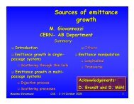
Example cavity tuned to 150 MHz 


Can Superfish do travelling waves? 

here a hint on a paper tissue ... 


3 rd 

exercise: How to construct a TW solution from a SW solution? 

Floquet’s theorem: 

For a periodic structure with period , Floquet’s theorem states that it has solutions 

that are similar from one period to the next, their difference can be characterized by 

just a complex factor. 

These solutions are the “modes” of the periodic structure (also “Bloch waves”). 

If we restrict ourselves to a lossless structure, then for a propagating mode the 

complex factor has the absolute value 1 and is characterized by just a rotation in 

j 

phase; for this reason, let us write the factor as e . 

It describes the field of a forward travelling wave. 

j 

Floquet’s theorem further states that if there is a solution e , there is also the 

j 

complex conjugate solution e . The complex conjugate of the above describes the 

backward travelling wave: 

 

is the phase advance per cell. 

f 

f 

j 

z 

f ze * j 

z 

f ze * 


Standing wave 

If you superimpose a forward travelling and a backward travelling wave with the 

same amplitude, you obtain a standing wave. Superfish will calculate standing 

waves. If will be a real function of z: 

s 

* 

z f z f z We will now try to invert the above thoughts and try to extract the complex 

function f z from the real function sz 

that we have obtained from Superfish. 

We can use our knowledge about the periodicity of f z , since the Superfish 

solution for the field is known for more than one period; the real solution in the 

next cell is also known: 

j * j 

s z f z e f z e 

 

Multiplying the 1st equation with and subtracting the 2nd j 

e 

gives: 

This can be solved for 

s 

j j 

j 

zszefze e 

f 

z 

s 

z 

sz 

j 

j 

e 

e 


e 

j 

.

Example: CTF3 DBA 

3 cells, 3 GHz DBA Structure 

&reg kprob=1, dx=0.0400, 

freq=2999.5500,icylin=1.0000,irtype=2,rho=0, 

kmethod=1,beta=1,zctr=4.9980& 

&po x=0.0000,y=0.0000& 

Here (simplified) 3 cells of the drive beam 

&po x=9.9960,y=0.0000& 

&po x=9.9960,y=1.7000& 

accelerator of CTF3, the CLIC Test Facility at CERN. &po x=9.5300,y=1.7000& 

&po x=9.5096,y=2.2993,nt=5,radius=0.3000& 

&po x=9.6960,y=2.4988,nt=4,radius=0.2000& 

Shown below is the standing wave pattern 

&po x=9.6960,y=3.5245& 

&po x=9.4960,y=3.7245,nt=4,radius=0.2000& 

obtained by the superposition of two counter‐ 

&po x=7.1640,y=3.7245& 

&po x=6.9640,y=3.5245,nt=4,radius=0.2000& 

running 2π/3‐modes and the axial field on axis. 

&po x=6.9640,y=2.4988& 

&po x=7.1504,y=2.2993,nt=4,radius=0.2000& 

&po x=7.1300,y=1.7000,nt=5,radius=0.3000& 

&po x=6.6640,y=1.7000& 

&po x=6.1980,y=1.7000& 

&po x=6.1776,y=2.2993,nt=5,radius=0.3000& 

&po x=6.3640,y=2.4988,nt=4,radius=0.2000& 

&po x=6.3640,y=3.5245& 

&po x=6.1640,y=3.7245,nt=4,radius=0.2000& 

&po x=3.8320,y=3.7245& 

&po x=3.6320,y=3.5245,nt=4,radius=0.2000& 

&po x=3.6320,y=2.4988& 

&po x=3.8184,y=2.2993,nt=4,radius=0.2000& 

&po x=3.7980,y=1.7000,nt=5,radius=0.3000& 

&po x=3.3320,y=1.7000& 

&po x=2.8660,y=1.7000& 

&po x=2.8456,y=2.2993,nt=5,radius=0.3000& 

&po x=3.0320,y=2.4988,nt=4,radius=0.2000& 

&po x=3.0320,y=3.5245& 

&po x=2.8320,y=3.7245,nt=4,radius=0.2000& 

&po x=0.5000,y=3.7245& 

&po x=0.3000,y=3.5245,nt=4,radius=0.2000& 

&po x=0.3000,y=2.4988& 

&po x=0.4864,y=2.2993,nt=4,radius=0.2000& 

&po x=0.4660,y=1.7000,nt=5,radius=0.3000& 

&po x=0.0000,y=1.7000& 

&po x=0.0000,y=0.0000& 


The modes of the 3‐cell closed structure: 

0‐mode: 2.938 GHz 

π/3‐mode: 2.959 GHz 

2π/3‐mode: 2.999 GHz 

π‐mode: 3.019 GHz 


Reconstructing the travelling wave: 

Extract the field on axis: to this end, you call 

the interpolation program SF7, which can 

extract the field *) . To start it, right‐click on the 

T35‐file (“Poisson Superfish Solution”) and 

select “Interpolate (SF7)” from the pull‐down 

menu; you will see the window shown here. 

Select the axis! This will create the file 

“OUTSF7.TXT” from which you can read with 

another program (I used Mathematica). The 

axial field on the axis looks like this: 

*) During the lecture, I showed a different, more difficult way, so I’d like to 

acknowledge Ciprian Plostinar, who pointed this more elegant solution out to me! 


Mathematica implementation: 

Here now a possible Mathematica 

implementation to solve f 

z z 

sz 

j 

j 


 

s 

e 

e 

e 

j

Cavity Basics - CERN Accelerator School

You also want an ePaper? Increase the reach of your titles

Delete template?

Save as template?