steady laminar couette flow of a dilatant fluid along a channel with ...

J. Hydrol. Hydromech., 52, 2004, 3, 175–184
STEADY LAMINAR COUETTE FLOW OF A DILATANT FLUID
ALONG A CHANNEL WITH SUCTION AT A BOUNDING WALL
N. C. SACHETI l) , P. CHANDRAN 1) , R. P. JAJU 2) and B. S. BHATT 3)
1)
Department of Mathematics and Statistics, College of Science, Sultan Qaboos University, P. O. Box 36, PC 123, Al Khod, Muscat,
Sultanate of Oman.
2)
Department of Computer Science, University of Swaziland, Kwaluseni, Swaziland.
3)
Department of Mathematics, The University of West Indies, St. Augustine, Trinidad, West Indies.
1. Introduction
We consider a special dilatant fluid model for which the apparent viscosity can be expressed as a polynomial
in the second scalar invariant of the rate of strain tensor. The model has been used to investigate the
steady plane Couette flow of a non-Newtonian fluid through a channel with suction, assumed small, at the
lower porous wall. The introduction of a similarity transformation in the perturbed governing partial differential
equations of the flow leads to a system of coupled non-linear ordinary differential equations. The solutions
of these equations have been obtained analytically as a power series in the suction parameter λ. The
combined effects of the non-Newtonian and the suction parameters on the longitudinal and transverse velocity
profiles as well as the skin friction, have been discussed. The validity of the analytical solutions has also
been checked with the corresponding numerical solutions for small values of the governing parameters.
KEY WORDS: Non-Newtonian Fluid, Plane Couette Flow, Similarity Transformation, Suction, Skin Friction.
N. C. Sacheti, P. Chandran, R. P. Jaju, B. S. Bhatt: USTÁLENÉ LAMINÁRNE COUETTEHO
PRÚDENIE NENEWTONSKEJ TEKUTINY V POTRUBÍ SO SANÍM NA STENÁCH. Vodohosp. Čas.,
52, 2004, 3; 23 lit., 2 obr., 1 tab.
Štúdia sa zaoberá sa špeciálnym modelom nenewtonskej tekutiny, pre ktorú sa môže skutočná viskozita
vyjadriť vo forme polynomickej závislosti na druhom skalárnom invariante tenzora rýchlosti deformácie.
Model bol využitý na štúdium ustáleného Couetteho rovinného prúdenia nenewtonskej tekutiny v kanáli so
saním cez porézne steny. Zavedenie transformácie podobnosti do lineanizovaných parciálnych diferenciálnych
rovníc vedie k systému obyčajných nelineárnych diferenciálnych rovníc. Ich riešenie sme získali vo
forme potenčného radu od sacieho parametra λ. Analyzovali sme vplyv rozťažnosti tekutiny a sacieho parametra
na pozdĺžny a priečny rýchlostny profil, ako aj na povrchové trenie. Platnosť analytického riešenia
sme porovnali s numerickým riešením pre malé hodnoty použitých parametrov.
KĽÚČOVÉ SLOVÁ: Nenewtonská tekutina, rovinné prúdenie Couette, transformácia podobnosti, sanie,
povrchové trenie.
The flow of viscous fluids in the presence of porous
boundaries has been a subject of intense investigations
in the last five decades or so due to numerous
applications. For instance, the liquid coolants
which exude through the porous walls with
uniform porosity, are known to play vital roles in
the transpiration cooling of the head of missiles and
re-entry bodies. The suction or injection of fluids
through permeable walls also find useful applications
in industries. Furthermore, the study of flow
problems involving suction or injection of fluids at
the walls of channels, pipes and annuli becomes
important because of their significant effects on
axial pressure gradients, velocity profiles of flow
and wall stresses. As a result, a large number of
analytical studies on viscous flow has been reported
in the literature. Following Berman (1953), several
researchers, (see, e.g., Yuan and Finkelstein, 1956;
Cramer, 1959; Lilley, 1959; Terrill and Shrestha,
1965; Verma and Bansal, 1966; Masuzawa et al.,
1980; Zatursta et al., 1988; Cox, 1991), analyzed
steady laminar flow of Newtonian fluids through
channels and pipes. In most investigations, the suction
or injection of the fluid has been assumed to be
175

N. C. Sacheti, P. Chandran, R. P. Jaju, B. S. Bhatt
normal to the porous walls of same or different
permeabilities, although some researchers have also
considered oblique suction (Weidman and Amberg,
1996). The analytical solutions in these studies
have generally been obtained under the assumption
that the suction or injection Reynolds number is
small.
On the other hand, several investigators have extended
the viscous flow problems mentioned above
to non-Newtonian fluids, apparently because of
increasing technological applications of rheological
fluids. In doing so, a number of non-Newtonian
fluid models has been proposed in the literature
(Narasimhan, 1961; Rajvanshi, 1968; Bhatnagar,
1971; Sacheti, 1976; Sacheti and Bhatt, 1976; Ariel,
1992). However, the analysis of the flow of non-
Newtonian fluids through porous channels or pipes
presents mathematical difficulties because of the
non-linearity of the governing equations. Recently,
Ariel (2002) has discussed steady laminar flow of a
second grade fluid through two parallel porous
walls, and obtained exact analytical solutions as
well as perturbation solutions, assuming that the
rate of injection at one wall is equal to the rate of
suction at the other wall. The present investigation
considers the extension of a classical Couette flow
problem with small suction at the lower wall, to a
special dilatant fluid model which has received
relatively less attention in the literature. Our main
objective is thus to discuss the effect of wall porosity
on the ensuing non-Newtonian flow.
2. The fluid model and the governing equations
As is known, a constitutive equation of an inelastic
non-Newtonian fluid can be represented as (Bird
et al., 1960)
τ µ
ij = ( I1, I2, I3) eij
, (1)
where I 1,
I 2 and I 3 are the scalar invariants of the
rate of strain tensor. For two-dimensional flow, as
is being considered in the present study, I 1 and I 3
vanish identically so that µ becomes a function of
I 2 only. We furthermore assume that µ can be
approximated as a power series in I 2 , and write
176
2
2 0 1 2 2 2
µ ( I ) = µ + µ I + µ I + ...,
(2)
where µ 0 is the conventional Newtonian viscosity,
while the parameters µ 1 , µ 2 , ⋯ , indicate the non-
Newtonian character of the fluid. In the present
study, we consider the fluid model with the constitutive
equation
τ µ µ
ij = ( 0 + 1I2) eij.
(3)
Eqs. (2) and (3) allow us to account for the shearthickening
behaviour of the inelastic fluid. The
model described by Eq. (3) and a model with the
higher order effect had recently been employed to
study the stagnation point flow near a stationary
impermeable wall (Sacheti et al., 2000, 2003). In
the present work, the model given by Eq. (3) is
used to analyze the plane Couette flow subject to
suction at the lower boundary.
We thus consider the steady, laminar flow of the
inelastic fluid in a channel bounded by two infinite
parallel plates distant h apart. In the Cartesian coordinate
system, with a suitably chosen origin, the
x -axis is taken along the stationary lower porous
plate, while the y-axis is taken perpendicular to it
into the fluid. Let u( xy , ) and v( xy , ) denote the
fluid velocities in the x and y directions, respectively.
The upper plate, y= h,
is assumed to be
moving with a uniform velocity U in the xdirection.
In addition, the fluid flow is subject to a
uniform suction given by v =− v0
at the stationary
plate y = 0. Under the assumption of constant density
ρ of the fluid, the equations governing the
velocity components u( xy, , ) v( xy , ) and the pressure
pxy ( , ) are the usual equations of continuity
and momentum, and are given by
∂u ∂v
+ = 0,
∂x ∂y
⎛ ∂u ∂u⎞ ∂p
∂τ
∂τ
ρ u v
xx
⎜ + ⎟ = − + +
⎝ ∂x ∂y⎠ ∂x ∂x ∂y
⎛ ∂v ∂v⎞ ∂p
∂τ∂τ ρ ⎜u + v ⎟ = − + +
⎝ ∂x ∂y⎠ ∂y ∂x ∂y
xy
xy yy
,
.
(4)
(5)
(6)
On using the rheological model (3), Eqs. (5) and (6)
can be shown to transform to

2 2
⎛ ∂u∂u⎞ ∂p ⎛∂ u ∂ u⎞
ρ ⎜u + v ⎟ = − + µ 0 ⎜ + ⎟
x y x 2 2
⎝ ∂ ∂ ⎠ ∂ ⎜∂x ∂y
⎟
⎝ ⎠
2 2
⎛∂u⎞ ∂ u
+ 16µ
1 ⎜ ⎟
⎝∂x⎠ 2
∂x
⎧ 2 2 2 2
⎪ u u v
⎫⎛ ⎛∂ ⎞ ⎛∂ ∂ ⎞ ⎪ ∂ u ∂ u⎞
1 ⎨4⎜ ⎟ ⎬⎜
⎟
2 2
+ µ ⎜ ⎟ + + +
⎝∂x⎠ ⎝∂y ∂x⎠
⎜∂x ∂y
⎟
⎩⎪ ⎭⎪⎝
⎠
2 2 2
⎛∂u ∂v⎞ ⎛∂ u ∂ u⎞
+ 2µ
1 ⎜ + ⎟ ⎜ − ⎟
y x 2 2
⎝∂ ∂ ⎠
⎜∂y ∂x
⎟
⎝ ⎠
2 2
2 ,
⎛ u ∂ v⎞
⎜ + ⎟
∂u⎛∂u ∂v⎞ ∂
+ 4µ 1 ⎜ + ⎟ 3
∂x⎝∂y ∂x⎠
⎜ ∂∂ xy ∂x
⎟
⎝ ⎠
2 2
⎛ ∂v∂v⎞ ∂p ⎛∂ v ∂ v⎞
ρ ⎜u + v ⎟ = − + µ 0 ⎜ + ⎟
x y y 2 2
⎝ ∂ ∂ ⎠ ∂ ⎜∂x ∂y
⎟
⎝ ⎠
2 2
⎛∂ ⎞ ∂
− 16µ
1 ⎜ ⎟
u u
⎝∂x⎠ ∂y∂x ⎧ 2 2 2 2
⎪ u u v
⎫⎛ ⎛∂ ⎞ ⎛∂ ∂ ⎞ ⎪ ∂ v ∂ v⎞
1 ⎨4⎜ ⎟ ⎬⎜
⎟
2 2
+ µ ⎜ ⎟ + + +
⎝∂x⎠ ⎝∂y ∂x⎠
⎜∂x ∂y
⎟
⎩⎪ ⎪⎝ ⎭
⎠
2 2 2
⎛∂u ∂v⎞ ⎛∂ v ∂ v⎞
+ 2µ
1 ⎜ + ⎟ ⎜ − ⎟
y x 2 2
⎝∂ ∂ ⎠
⎜∂x ∂y
⎟
⎝ ⎠
∂u⎛∂u ∂v⎞⎛ 2 2
∂ u ∂ u⎞
+ 4µ 1 ⎜ + ⎟⎜3
− ⎟
∂x⎝∂y ∂x⎠
⎜ ∂x ∂y
⎟
⎝ ⎠
Steady laminar Couette flow of a dilatant fluid along a channel wth suction at a bounding wall
2 2 .
(7)
(8)
The Couette flow is subject to the boundary conditions
u = 0, v=−v0at y = 0; u = U, v= 0 at y = h.
(9)
Since there is a uniform suction all along the stationary
lower plate, we have, ∂v/ ∂ x = 0, and from
the equation of continuity it follows that
2 2
∂ u/ ∂ x = 0. Using these results in Eqs. (7) and
(8), we obtain
⎛ ∂u ∂u⎞ ∂p ⎜u + v ⎟ = − +
⎝ ∂x ∂y⎠ ∂x 2
∂ u
0 2
∂y
⎡
µ 1 ⎢
⎢⎣ 2 2
∂ u⎛∂u⎞ 2 ⎜ ⎟
∂y ⎝∂x⎠ ∂u⎛ ⎜
∂y⎜ ⎝
2
∂u ∂ u
∂x ∂y∂x 2
∂u ∂ u⎞⎤
⎟⎥
∂y
2
∂y
⎟
⎠⎥⎦
ρ µ
+ 4 + 3 4 + ,
(10)
2
0 2
∂v ∂p ∂ v
ρ v =− + µ
∂y ∂y ∂y
⎡ 2 2 2 2
∂u⎛∂u ∂ u ∂u ∂ u⎞ ∂ u ⎛∂u⎞ ⎤
1 ⎢ ⎜ ⎟
y y x y x 2
⎜ ⎟ ⎥
⎢ ∂ ⎜∂ ∂ ∂ ∂ y ⎟ ∂x∂y⎝∂x ⎣ ⎝ ∂ ⎠
⎠ ⎥⎦
+ µ
− 4 − 20 .
(11)
Eqs. (4), (10) and (11) are the ones that will be
used in our flow analysis. We shall nondimensionalize
these equations by introducing the
non-dimensional quantities
u = u/ U, v = v/ U, x = x/ h, η = y/ h,
2
(12)
p = p/ ρU , λ = ρ hv / µ , R = ρ Uh/
µ .
( )
0 0 0
In the above, λ is the suction parameter and R is
the Reynolds number corresponding to the zero
shear viscosity µ 0 . Using Eq. (12), Eqs. (4), (10)
and (11) can be expressed, respectively, in the nondimensional
forms
∂u ∂v
+ = 0,
∂x∂η (13)
2
∂u ∂u ∂p 1 ∂ u
u + v = − +
∂x ∂η∂x R 2
∂η
2 2
2 2
K ⎡ ∂ u ⎛∂u ⎞ ∂u ⎛ ∂u ∂ u ∂u ∂ u ⎞⎤
+ ⎢4 3 4 ,
R 2 ⎜ ⎟ + ⎜ + ⎟⎥
x η x η x η 2
⎢ η ⎝∂ ⎠ ∂ ⎜ ∂ ∂ ∂ ∂ η ⎟
⎣ ∂ ⎝ ∂ ⎠⎥⎦
(14)
2
∂v ∂p 1 ∂ v
v =− +
∂η ∂η R 2
∂η
2 2 2 2
K ⎡ ∂u ⎛∂u ∂ u ∂u ∂ u ⎞ ∂ u ⎛∂u ⎞ ⎤
+ ⎢ ⎜ −4⎟−20 ⎥,
R η η x η x 2
⎜ ⎟
⎢∂ ⎜∂ ∂ ∂ ∂ η ⎟ ∂x∂η⎝∂x ⎣ ⎝ ∂ ⎠
⎠ ⎥⎦
(15)
2 2
where K = µ 1U /( µ 0h
) is a parameter characterizing
the ratio of non-Newtonian and Newtonian
effects. The boundary conditions in terms of the
non-dimensional quantities are
u = 0, v = − λ/R at η = 0;
(16)
u = 1, v = 0 at η = 1.
We now write
p( x, η) = p0+ p̃ ( x, η), u( x,
η)
=
= u + ũ( x, η), v( x, η) = ṽ( x,
η),
0
(17)
177

N. C. Sacheti, P. Chandran, R. P. Jaju, B. S. Bhatt
where the quantities with a tilde are the perturbations
caused by the suction, and p 0 , u 0 are the
known quantities for the plane Couette flow satisfying
the conditions
178
0 0 0
2
0
2
∂p ∂p ∂u ∂ u
= 0, = 0, = 0, = 0.
∂x ∂η∂x ∂η
We thus have
(18)
p 0 = constant, and u0 = η . (19)
In the following, we shall suppress the tilde in the
perturbed quantities, for convenience. Using Eqs.
(17) and (18) in Eqs. (13) – (15), the equations
governing the perturbed velocity components and
pressure can be written as
∂u ∂v
+ = 0
∂x∂η 2
∂u ∂u ∂u ∂p 1 ∂ u
u0+ u + v = − +
∂x ∂x ∂η∂x R 2
∂η
2 2 2
4K ⎛∂u⎞ ∂ u 12K
⎛ ∂u ⎞∂u
∂ u
+ ⎜ ⎟ + 1
R x 2 ⎜ + ⎟
⎝∂ ⎠ ∂η R ⎝ ∂ ⎠∂x
∂x∂ 2 2
3K
⎛ ∂u ⎞ ∂ u
+ ⎜1+ ⎟
R η 2
⎝ ∂ ⎠ ∂η
η η
(20)
(21)
2 2 2
∂v∂p 1 ∂ v 20K
⎛∂u⎞ ∂ u
v =− + −
R 2 ⎜ ⎟
∂η∂η ∂η
R ⎝∂x ⎠ ∂x∂η 2 2 2
4K
⎛ ∂u ⎞∂u ∂ u K ⎛ ∂u ⎞ ∂ u
− ⎜1+ ⎟ + 1 .
R η x 2 ⎜ + ⎟
⎝ ∂ ⎠∂ ∂η
R ⎝ ∂η ⎠ ∂x∂η (22)
In terms of the perturbed quantities, the boundary
conditions now become
u = 0, v = − λ/ R at η = 0;
(23)
u = 0, v = 0 at η = 1.
3. Method of solution
∂p 1
2
= ⎡F′′ − λη ( f′ + F f′ − f − fF′ ) + 3 K(1 + F′ ) F′′
⎤
∂x
R ⎣ ⎦
λx
2 2
+ ⎡f′′′ −λ( f′ − f f′′ ) + 6 Kf′′ F′′ (1 + F′ ) + 3 Kf′′′ (1 + F′
) ⎤
2
R ⎣ ⎦
2 2 2
4Kλ 2 3Kλ
x
2
+ ⎡f′ F′′ + 3(1 + F′ ) f′ f′′ ⎤ + ⎡2(1 + F′ ) f′′ f′′′ + f′′ F′′
⎤
3 3
R ⎣ ⎦ R ⎣ ⎦
3 3 3
4Kλ x
⎡ 2 2 3Kλ
x
f′ f′′′ 3 f′′ f′ ⎤ f′′
2
+ + +
f ′′′ ,
4 4
R ⎣ ⎦ R
∂p
λ
2
= ⎡Kf ′′ (1 + F′ ) − 4 K f ′ F′′ (1 + F′ ) −λff′ − f ′′ ⎤
∂η
2
R ⎣ ⎦
2
2Kλx
2
+ ⎡(1 + F′ )( f′′ −2 f′ f′′′ ) −2f′
f′′ F′′
⎤
3
R ⎣ ⎦
3 2 3
Kλ x 3 20Kλ
2
+ ⎡f′′ −4 f′ f′′ f′′′ ⎤ − f′ f′′
.
4 4
R ⎣ ⎦ R
In order to obtain a coupled system governing
the functions f and F , we use the result
We assume that the transverse velocity v can be
expressed as
λ
v =− f ( η)
(24)
R
so that, from Eq. (20), the longitudinal velocity
takes the form
λ
u = xf′ ( η) + F(
η),
(25)
R
where f ( η ) and F( η ) are unknown functions to
be found. Using the above functional expressions of
u and v in Eqs. (21) and (22), we obtain
∂p/ ∂ x = 0 at x = 0 in Eq. (26), and this yields
(26)
(27)

2
F′′ − λη ( f′ + F f′ − f − f F′ ) + 3 KF′′ (1 + F′
)
2
Kλ
(28)
2
+ ⎡4f′ F′′ + 12 f′ f′′ (1 + F′
) ⎤ = 0.
2
R ⎣ ⎦
( ′′ ′′′ ′′ ′′′′ )
Steady laminar Couette flow of a dilatant fluid along a channel wth suction at a bounding wall
f′′′′ − λ(
f′ f′′ − f f′′′ ) + 6K f′′ F′′ + 3 K(1 + F′ )(4f′′′ F′′ + 2 f′′ F′′′
)
2 2 2 3
+ 3 K(1 + F′ ) f′′′′ + 2 K( λ / R) (20 f′ f′′ f′′′ + 2 f′ f′′′′ + 5 f′′
)
2 2
+ 3 K( λx/
R) ⎡4 f′′ f′′′ F′′ + 2(1 + F′ )( f′′′ + f′′ f′′′′ + f′′ F′′′
) ⎤
⎣ ⎦
2
+ 3 K( λx/
R) 2 f f
2
+ f
2
f = 0.
Eqs. (28) and (29) are highly nonlinear, and cannot
be solved analytically. However, it is of practical
interest if one can obtain analytical solutions of
these equations subject to certain restrictive assumptions.
To this end, we assume that the non-
Newtonian parameter K is small (

N. C. Sacheti, P. Chandran, R. P. Jaju, B. S. Bhatt
2
f2′′′′ + f0′′ f1 − f0′′ f1′ − f0′ f1′′ + f0 f1′′′ + 6K
f0′′ F1′′
+ 3 K[4 f0′′′ F1′ F1′′ + 4 f1′′′ F1′′ + 4 f0′′′ F2′′ + 2 f0′′ F1′ F1′′′ + 2 f0′′ F2′′′
2
+ 2 f1′′ F1′′′ + 2 f0′′′′ F2′ + 2 f1′′′′ F1′ + f0′′′′ F1′ + f2′′′′
] = 0.
The boundary conditions to be satisfied by the
functions i f and F i are
fi(1) = 0, fi′ (0) = 0, fi′ (1) = 0, ( i = 0, 1, 2),
(40)
f0(0) = 1, fi(0) = 0, ( i = 1, 2),
Fi(0) = Fi(1) = 0, ( i = 1, 2).
(41)
Eqs. (35) – (39), subject to the boundary conditions
(40) and (41), can be solved analytically. The solutions
have been obtained in powers of (small) K .
They can be expressed as
180
= 1 + 2 + 3 +
2
4
2
[ L5( ) KL6( )
2
K L7(
)],
f( η) L ( η) λ[ L ( η) KL ( η) K L ( η)]
+ λ η + η + η
= − +
2
1
2
M2 KM3 2
K M4
F( η) λ(1 3K 9 K ) M ( η)
+ λ [ ( η) + ( η) + ( η)],
(42)
(43)
where Li( η ), ( i=
1,2,...,7), and Mi( η ), ( i = 1,2,3,
4), are polynomials in η . Explicit expressions of
these polynomials are given in Appendix I. Using
Eqs. (42) and (43), analytical expressions for the
velocity components u and v can be obtained.
While the emphasis of this work has been on carrying
out analytical studies of the fluid motion, the
non-linear boundary value problem described by
Eqs. (30) – (32) has also been solved numerically
using a “shooting method”. As before, the resulting
values of the functions f and F have been used to
calculate the velocity components u and v .
4. Results
The analytical solutions of the perturbed functions
f and F given by Eqs. (42) and (43) can be
employed in Eqs. (24) and (25) to obtain the perturbed
velocity components. These, in conjunction
with Eqs. (17) and (19), yield the non-dimensional
longitudinal and transverse components of velocity.
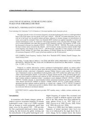
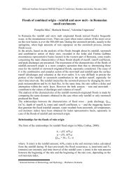
We have compared the analytical solutions for a set
of values of the perturbation parameter λ with the
corresponding numerical solutions. The results are
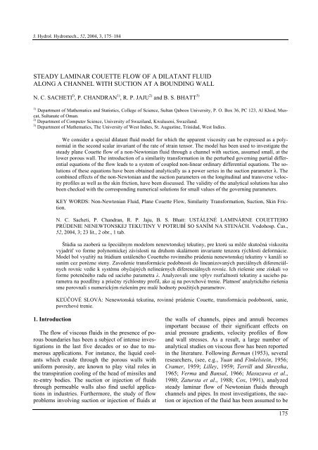
shown in Figs 1 and 2. The plots correspond to the
(39)
variations of the velocity components at the channel
cross section x = 20, for the fixed value of the non-
Newtonian parameter, K = 0.2, and the Reynolds
number, R = 50. In the Figure 1, the longitudinal
velocity profiles have been compared for the cases
λ = 0.3 and λ = 0.6, while the Figure 2 gives the
corresponding results for the transverse component
of the velocity. It may be observed that the analytical
and numerical results compare quite favourably
for λ = 0.3.
However, for higher values of λ , the
corresponding velocity profiles seem to show enhanced
deviation – this expected deviation is due to
the perturbation approximation involving the parameter
λ . For λ = 0, the longitudinal velocity
profile can be seen to be the well known linear one,
while the velocity profiles for non-zero values of λ
– both longitudinal and transverse – exhibit deviations
from the classical plane Couette flow. It is
also worth observing that the magnitudes of the
velocity components decrease with λ . The deviations
of the velocity profiles are maximum in the
central region of the channel, see Fig. 1.
In most applications involving rheological fluids,
it is of interest to make predictions of the effects of
non-Newtonian parameters on the local wall shear
stress ( τ xy at y = 0 in the present case). For our
model the non-dimensional skin friction coefficient,
C f , is given by
2
C f = A(1 + KA ) , (44)
where
A = 1 + ( λ x/ R) f′′ (0) + F′
(0).
The computed values of C f based on the analytical
solutions have been given in Tab. 1, for x = 20 and
R = 50. From Tab. 1, we observe that, for a fixed
value of the non-Newtonian parameter K , the wall
shear stress decreases with increase in the suction.
However, the skin friction shows a mixed trend
when both parameters, K and λ , are allowed to
vary. It is noticed that for relatively low values of
λ ( ≈ 0.20), the skin friction coefficient increases
with the increase of the non-Newtonian parameter

Steady laminar Couette flow of a dilatant fluid along a channel wth suction at a bounding wall
Fig. 1. Variation of the longitudinal velocity u . ( K = 0.2, R = 50, x = 20) .
Obr. 1. Priebeh pozdĺžnej rýchlosti u, ( K = 0.2, R = 50, x = 20) .
Fig. 2. Variation of the transverse velocity v . ( K = 0.2, R = 50, x = 20) .
Obr. 2. Priebeh priečnej rýchlosti v, ( K = 0.2, R = 50, x = 20) .
181

N. C. Sacheti, P. Chandran, R. P. Jaju, B. S. Bhatt
K . But for higher values of λ , the skin friction
coefficient shows the reverse trend as K increases.
In other words, the usually observed phenomenon
of higher frictional force at an impermeable boundary
due to the non-Newtonian character of the fluid
(Sacheti et al., 2000) could be overcome by imposing
larger suction at a porous boundary. In such
cases of larger values of the suction and non-
Newtonian parameters (falling within our perturbation
range), there is also a tendency for the fluid to
undergo back-flow near the porous plate, see, for
instance, the profiles in Fig.1.
T a b l e 1. Values of the skin friction coefficient C f , R = 50,
x = 20 .
T a b u ľ k a 1. Hodnoty koeficienta povrchového trenia Cf, R = 50, x = 20 .
182
λ
0.00
0.05
0.10
0.15
0.20
0.25
0.30
0.35
0.40
0.45
0.50
0.55
0.60
5. Summary
C f
K = 0.0 K = 0.1
1.0000
0.9073
0.8143
0.7210
0.6273
0.5332
0.4387
0.3438
0.2485
0.1527
0.0565
-0.0403
-0.1375
1.1000
0.9758
0.8580
0.7455
0.6373
0.5327
0.4307
0.3305
0.2313
0.1324
0.0328
-0.0684
-0.1719
K = 0.2 K = 0.3
1.2000
1.0482
0.9076
0.7752
0.6484
0.5249
0.4027
0.2795
0.1530
0.0205
-0.1220
-0.2796
-0.4594
1.3000
1.1277
0.9673
0.8132
0.6616
0.5092
0.3535
0.1907
0.0151
-0.1841
-0.4270
-0.7484
-1.2066
The class of non-Newtonian fluids exhibiting
dilatant behaviour has attracted the attention of
researchers in recent years, mainly due to their
increasing applicability in the processing of
highly concentrated suspensions and pastes. We
have thus considered the steady laminar Couette
flow of a special class of dilatant fluids through a
straight channel subject to small suction at the
lower boundary. We have carried out the flow
analysis as a perturbation to the classical plane
Couette flow, and obtained a set of two highly
non-linear partial differential equations in the
perturbed flow variables. These equations have
been subjected to a similarity transformation and
the resulting ordinary differential equations have
been analyzed under certain assumptions on the
governing parameters. This procedure has en-
abled us to obtain power series solutions of the
similarity functions. In order to assess the usefulness
of the power series solutions, we have computed
the analytical solutions, and then compared
them with the numerical solution of the relevant
non-linear boundary value problem. It has been
noticed that the solutions for small values of the
suction parameter are in good agreement with the
corresponding numerical solutions. The influence
of suction on the velocity profiles as well as the
drag at the porous boundary has been analyzed. It
has been shown that they both decrease with suction.
There is also a tendency for the fluid to undergo
back-flow near the porous boundary, as the
suction is increased.
List of symbols
A – dimensionless quantity defined in Eq. (44),
C – dimensionless skin friction coefficient,
f
e ij – rate of strain tensor [T -1 ],
f, F – dimensionless functions in Eqs (24) and (25),
2h – channel width [ L ] ,
I 1 – first invariant of the rate of strain tensor
I 2 – second invariant of the rate of strain tensor
I 3 – third invariant of the rate of strain tensor
K – dimensionless non-Newtonian parameter,
L M – dimensionless functions of η ,
,
i i
−1−2 p – fluid pressure [ ML T ] ,
R – Reynolds number [–],
u, v –
1
fluid velocity components [ LT ]
−
,
1
U – velocity of upper plate [ LT ]
−
,
v 0 – suction velocity at the lower plate
1
[ LT ]
−
,
x, y – space coordinates [ L ] ,
x – dimensionless longitudinal coordinate,
η – dimensionless transverse coordinate,
λ – dimensionless suction parameter,
µ 0 – zero shear viscosity
−1−1 [ ML T ] ,
µ 1 – non-Newtonian parameter
3
ρ – fluid density [ ML ]
−
,
τ ij – stress tensor
REFERENCES
−1−2 [ ML T ] .
−1
[ ML T ] ,
1
[ T ]
−
,
2
[ T ]
−
,
3
[ T ]
−
,
ARIEL P.D., 1992: A hybrid method for computing the flow of
viscoelastic fluids. Int. J. Numer. Meth. Fluids, 14, 757.
ARIEL P.D., 2002: On exact solutions of flow problems of a
second grade fluid through two parallel porous walls. Int. J.
Engng. Sci., 40, 913.

BEARD D.B. and WALTERS K., 1964: Elastico-viscous
boundary layer flows. I – Two dimensional flow near a
stagnation point. Proc. Camb. Philos. Soc., 60, 667.
BERMAN A. S., 1953: Laminar flow in channels with porous
walls. J. Appl. Phys., 24, 1232.
BIRD R.B., STEWART W.E. and LIGHTFOOT E.N., 1960:
Transport Phenomena. Wiley, New York.
BHATNAGAR R.K., 1971: Flow of viscoelastic fluid between
two parallel walls in relative motion with uniform suction at
the stationary wall. ZAMM, 51, 377.
COX S.M., 1991: Analysis of steady flow in a channel with
porous wall or with accelerating walls. SIAM J. Appl.
Math., 51, 429.
CRAMER K.R., 1959: A generalized porous wall Couette type
flow. J. Aero/Space Sci., 26, 121.
LILLEY G.M., 1959: On a generalized porous wall Couette
type flow. J. Aero/Space Sci., 26, 685.
MASUZAWA J., TANAHASHI T. and ANDO T., 1980: Flow
of the entrance region in a porous pipe. Bull. JSME, 23,
672.
NARASIMHAN M.N.L., 1961: Laminar non-Newtonian flow
in a porous pipe. Appl. Sci. Res. A, 10, 393.
RAJVANSHI S.C., 1968: Steady laminar flow of viscoelastic
fluid through parallel and uniformly porous walls of different
permeability. Indian J. Pure Appl. Phys., 6, 512.
SACHETI N.C.: 1976, Plane Couette flow of two immiscible
non-Newtonian fluids with uniform suction at the stationary
plate. Indian J. Pure Appl. Math., 7, 527.
SACHETI N.C. and BHATT B.S., 1976: Steady laminar flow
of a non-Newtonian fluid with suction or injection and heat
transfer through porous parallel discs. ZAMM, 56, 43.
SACHETI N.C. and CHANDRAN P., 1997: On similarity
solutions for three dimensional flow of second order fluids.
J. Phys. Soc. Jpn., 66, 618.
SACHETI N.C., CHANDRAN P. and EL-BASHIR T., 2003:
Higher order approximation of an inelastic fluid flow. J.
Phys. Soc. Jpn., 72, 964.
SACHETI N.C., CHANDRAN P. and JAJU R.P., 2000: On the
stagnation point flow of a special class of non-Newtonian
fluids. Phys. Chem. Liquids, 38, 95.
SARPKAYA T. and RAINEY P.G., 1971: Stagnation point
flow of a second order viscoelastic fluid. Acta Mech., 11,
237.
TERRILL R.M. and SHRESTHA G.M., 1965: Laminar flow
through parallel and uniform porous walls of different permeability.
ZAMP, 16, 470.
VERMA P.D. and BANSAL J.L., 1966: Flow of a viscous
incompressible fluid between two parallel plates, one in uniform
motion and other at rest with uniform suction at the
stationary plate. Proc. Indian Acad. Sci., 64, 385.
WEIDMAN P.D. and AMBERG M.F., 1996: Similarity solutions
for steady laminar convection along heated plates with
variable oblique suction: Newtonian and Darcian fluid flow.
Quart. J. Mech. Appl. Math., 49, 373.
YUAN S.W. and FINKELSTEIN A., 1956: Laminar pipe flow
with injection and suction through porous walls. J. Appl.
Mech., 78, 719.
ZATURSTA M.B., DRAZIN P.B. and BANKS W.H.H., 1988:
On the flow of a viscous fluid driven along a channel by
suction at porous walls. Fluid. Dyn. Res., 4, 151.
Steady laminar Couette flow of a dilatant fluid along a channel wth suction at a bounding wall
Received 30 October 2003
Scientific paper accepted 28 July 2004
USTÁLENÉ LAMINÁRNE COUETTEHO PRÚDENIE
NENEWTONSKEJ TEKUTINY V POTRUBÍ
SO SANÍM NA STENÁCH
N. C. Sacheti, P. Chandran, R. P. Jaju, B. S. Bhatt
V poslednom čase priťahovalo pozornosť výskumníkov
dilatačné správanie skupiny nenewtonských tekutín,
a to najmä pre ich stúpajúcu využiteľnosť v
spracúvaní vysoko koncentrovaných suspenzií a pást. V
štúdii sme uvažovali ustálené laminárne Couetteho
prúdenie dilatačnej tekutiny cez rovný kanál s malým
saním na dolnej stene. Analyzovali sme prúdenie linearizovaním
rovníc pre klasický rovinný typ Couette. Tieto
rovnice boli pomocou podobnostnej transformácie pretransformované
na systém nelineárnych obyčajných
diferenciálnych rovníc a analyzované za zjednodušujúcich
predpokladov pre použité parametre. Tento postup
umožnil získať riešenie vo forme potenčného radu pre
podobnostnú funkciu. Pre posúdenie užitočnosti tohto
riešenia sme ho porovnávali s numerickým riešením tejto
úlohy. Riešenia pre malé hodnoty sacieho parametra boli
v dobrej zhode s numerickým riešením úlohy. Analyzovali
sme vplyv sania na rýchlostný profil ako aj povrchové
trenie poréznej steny. Ukázalo sa, že oboje rastie s
rastom sania. Je tam tiež tendencia k spätnému prúdeniu
na poréznej hranici, ak sa sanie zväčšuje.
Zoznam symbolov
A – bezrozmerný parameter v rov. (44),
Cf – bezrozmerný koeficient povrchového trenia,
eij – tenzor rýchlosti deformácie [T -1 ],
f, F – bezrozmerné funkcie v rov. (24), (25),
2h – šírka kanála [L],
I1 – prvý invariant tenzora rýchlosti deformácie [T -1 ],
I2 – druhý invariant tenzora rýchlosti deformácie [T -2 ],
I3 – tretí invariant tenzora rýchlosti deformácie [T -3 ],
K – bezrozmerný nenewtonský parameter,
Li, Mi – bezrozmerné funkcie η,
p – tlak tekutiny [ML -1 T -2 ],
R – Reynoldsovo číslo,
u, v – zložky rýchlosti [L T -1 ],
U – rýchlosť hornej dosky [L T -1 ],
vo – sacia rýchlosť na dolnej stene [L T -1 ],
x, y, – priestorové súradnice [L],
x – bezrozmerná dĺžková súradnica,
η – bezrozmerná priečna súradnica,
λ – bezrozmerný sací parameter,
µ o – počiatočná viskozita [ML -1 T -1 ],
– nenewtonská viskozita [ML -1 T -1 ],
µ 1
ρ – špecifická hmotnosť[M L -3 ],
τij – tenzor napätia [ML -1 T -2 ].
183

N. C. Sacheti, P. Chandran, R. P. Jaju, B. S. Bhatt
Appendix I
The functions Li, ( i= 1, … , 7) and Mi, ( i= 1, … , 4) occurring in Eqs. (42) and (43) are defined below:
3 2
L1 ( η) = 2η − 3η + 1,
7 6 5 4 3 2
L2 ( η) = (1/70)(4η − 14η + 21η − 35η + 43η − 19 η ),
7 6 5 4 3 2
L3 ( η) =−(3/ 70)(44η − 98η + 63η − 175η + 333η − 167 η ),
7 6 5 4 3 2
L4 ( η) = (18/ 70)(20η − 42η + 21η − 70η + 145η − 74 η ),
11 10 9 8 7 6
L5 ( η) =−(1/ 646800)(448η − 2464η + 3080η + 12705η − 50424η + 83776η
5 4 3 2
− 99792η + 99330η − 64378η + 17719 η ),
11 10 9 8 7
L6 ( η) =−(1/107800)(42672η − 134904η + 181720η − 430485η + 1110912η
6 5 4 3 2
− 1239084η + 1303303η − 1845690η + 1189301η −177745
η ),
11 10 9 8 7
L7 ( η) = (3/ 215600)(660352η − 2050048η + 2239160η − 4131435η + 9514296η
6 5 4 3 2
184
− 9178400η + 12509112η − 23832270η + 18851030η −4581797
η ),
5 4 2
M1 ( η) = (1/ 20)(4η −5η − 10η + 11 η),
9 8 7 6 5 4
M 2(
η) =−(1/5040)(32η − 117η + 36η + 588η − 1116η + 807η
3 2
3
− 840η + 1386η −776
η),
9 8 7 6 5
M ( η) =−(1/ 25200)(11040η − 23490η + 14040η − 57960η + 111672η
4
4 3 2
− 58320η + 50400η − 83160η + 35778 η),
9 8 7 6 5
M ( η) = (1/ 2800)(6640η − 14715η + 8460η − 24780η + 47268η
4 3 2
− 22335η + 21000η − 34650η +
13112 η).