Secondary CMB Anisotropy - Wayne Hu's Tutorials
Secondary CMB Anisotropy - Wayne Hu's Tutorials
Secondary CMB Anisotropy - Wayne Hu's Tutorials

Create successful ePaper yourself
Turn your PDF publications into a flip-book with our unique Google optimized e-Paper software.
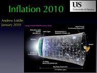
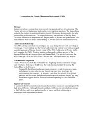
<strong>Secondary</strong> <strong>CMB</strong> <strong>Anisotropy</strong><br />
II: B-Modes & Lensing<br />
<strong>Wayne</strong> Hu<br />
Cabo, January 2009
Physics of <strong>Secondary</strong> Anisotropies<br />
SZ<br />
Primary Anisotropies<br />
Doppler<br />
ISW<br />
Vishniac<br />
Lensing<br />
Patchy rei.<br />
recombination<br />
z~1000<br />
reionization<br />
z~10<br />
acceleration<br />
z~1
∆ (µK)<br />
100<br />
10<br />
1<br />
0.1<br />
0.01<br />
Hu & Dodelson (2002)<br />
reionization<br />
Polarized Landscape<br />
ΘE<br />
gravitational<br />
waves<br />
10 100 1000<br />
l (multipole)<br />
EE<br />
BB<br />
gravitational<br />
lensing
B-mode Polarization
Electric & Magnetic Polarization<br />
(a.k.a. gradient & curl)<br />
• Alignment of principal vs polarization axes<br />
(curvature matrix vs polarization direction)<br />
Kamionkowski, Kosowsky, Stebbins (1997)<br />
Zaldarriaga & Seljak (1997)<br />
E<br />
B
Gravitational Waves
Quadrupoles from Gravitational Waves<br />
• Transverse-traceless distortion provides temperature quadrupole<br />
• Gravitational wave polarization picks out direction transverse to<br />
wavevector<br />
transverse-traceless<br />
distortion
Gravitational Wave Pattern<br />
• Projection of the quadrupole anisotropy gives polarization pattern<br />
• Transverse polarization of gravitational waves breaks azimuthal<br />
symmetry<br />
density<br />
perturbation<br />
gravitational<br />
wave
∆B (µK)<br />
Energy Scale of Inflation<br />
• Amplitude of B-mode peak scales as square of energy scale (Hubble<br />
parameter) during inflation, power as E i 4<br />
• Good: upper limits are at GUT scale. Bad: secondaries & foregrounds<br />
1<br />
0.1<br />
0.01<br />
10 100 1000<br />
l<br />
g-waves<br />
3<br />
E i (10 16 GeV)<br />
1<br />
0.3
The B-Bump<br />
• Rescattering of gravitational wave anisotropy generates the B-bump<br />
• Potentially the most sensitive probe of inflationary energy scale<br />
∆P (µK)<br />
10<br />
maximum<br />
amplitude!<br />
1<br />
reionization<br />
B-bump<br />
EE<br />
recombination<br />
B-peak<br />
10 100 1000<br />
l<br />
BB<br />
lensing<br />
contaminant
Slow Roll Consistency Relation<br />
• Consistency relation between tensor-scalar ratio and tensor tilt<br />
r = -8nt tested by reionization<br />
• Reionization uncertainties controlled by a complete p.c. analysis<br />
p.c.<br />
inst<br />
Mortonson & Hu (2007)
Patchy Reionization
Modulated Polarization<br />
• Ionization or density fluctuations modulate large angle E polarization<br />
into small angle E and B polarization
B-mode Contamination from Reionization<br />
• Inhomogeneous reionization modulates polarization into B-modes<br />
(Hu 2000)<br />
• Large signals if ionization bubbles >100Mpc at z~20-30<br />
Mortonson & Hu (2006)<br />
∆ l 2 [nK 2 ]<br />
10 5<br />
10 4<br />
10 3<br />
10 2<br />
10<br />
10<br />
500Mpc<br />
100 1000<br />
multipole l<br />
lensing<br />
50Mpc<br />
z i=30; τ=0.12<br />
Potentially removeable<br />
if large:<br />
Dvorkin & Smith (2008)
B-mode Contamination from Reionization<br />
• Inhomogeneous reionization modulates polarization into B-modes<br />
(Hu 2000)<br />
• Current expectation: grow to 10-100Mpc only at z
Gravitational Lensing
Example of <strong>CMB</strong> Lensing<br />
• Toy example of lensing of the <strong>CMB</strong> primary anisotropies<br />
• Shearing of the image
Gravitational Lensing<br />
• Gravitational lensing by large scale structure distorts the observed<br />
temperature and polarization fields<br />
• Exaggerated example for the temperature<br />
Original Lensed
Lensing by a Gaussian Random Field<br />
• Mass distribution at large angles and high redshift in<br />
in the linear regime<br />
• Projected mass distribution (low pass filtered reflecting<br />
deflection angles): 1000 sq. deg<br />
rms deflection<br />
2.6'<br />
deflection coherence<br />
10°
Lensing in the Power Spectrum<br />
• Lensing smooths the power spectrum with a width Δl~60<br />
• Convolution with specific kernel: higher order correlations<br />
between multipole moments – not apparent in power<br />
10 –10<br />
10 –11<br />
Power 10–9<br />
10 –12<br />
10 –13<br />
Seljak (1996); Hu (2000)<br />
lensed<br />
unlensed<br />
Δpower<br />
10 100 1000<br />
l
Gravitational Lensing<br />
• Lensing is a surface brightness conserving remapping of source to<br />
image planes by the gradient of the projected potential<br />
η0<br />
φ(ˆn) = 2 dη (D∗ − D)<br />
Φ(Dˆn, η) .<br />
D D∗<br />
such that the fields are remapped as<br />
η∗<br />
x(ˆn) → x(ˆn + ∇φ) ,<br />
where x ∈ {Θ, Q, U} temperature and polarization.<br />
• Taylor expansion leads to product of fields and Fourier<br />
mode-coupling
• Taylor expand<br />
Θ(ˆn) = ˜ Θ(ˆn + ∇φ)<br />
Flat-sky Treatment<br />
= ˜ Θ(ˆn) + ∇iφ(ˆn)∇ i ˜ Θ(ˆn) + 1<br />
2 ∇iφ(ˆn)∇jφ(ˆn)∇ i ∇ j ˜ Θ(ˆn) + . . .<br />
• Fourier decomposition<br />
φ(ˆn) =<br />
˜Θ(ˆn) =<br />
<br />
<br />
d2l φ(l)eil·ˆn<br />
(2π) 2<br />
d 2 l<br />
(2π) 2 ˜ Θ(l)e il·ˆn
Flat-sky Treatment<br />
• Mode coupling of harmonics<br />
<br />
Θ(l) = dˆn Θ(ˆn)e −il·ˆn<br />
where<br />
= ˜ Θ(l) −<br />
L(l, l1) = φ(l − l1) (l − l1) · l1<br />
+ 1<br />
2<br />
d 2 l1<br />
(2π) 2 ˜ Θ(l1)L(l, l1) ,<br />
d 2 l2<br />
(2π) 2 φ(l2)φ ∗ (l2 + l1 − l) (l2 · l1)(l2 + l1 − l) · l1 .<br />
• Represents a coupling of harmonics separated by L ≈ 60 peak of<br />
deflection power
• Power spectra<br />
becomes<br />
C ΘΘ<br />
l<br />
where<br />
Power Spectrum<br />
〈Θ ∗ (l)Θ(l ′ )〉 = (2π) 2 δ(l − l ′ ) C ΘΘ<br />
l<br />
〈φ ∗ (l)φ(l ′ )〉 = (2π) 2 δ(l − l ′ ) C φφ<br />
l ,<br />
= 1 − l 2 R ˜ C ΘΘ<br />
l<br />
+<br />
R = 1<br />
4π<br />
d 2 l1<br />
(2π) 2 ˜ C ΘΘ<br />
|l−l1|C φφ<br />
l1 [(l − l1) · l1] 2 ,<br />
dl<br />
l l4 C φφ<br />
l .<br />
,
• If ˜ C ΘΘ<br />
l<br />
Smoothing Power Spectrum<br />
slowly varying then two term cancel<br />
˜C ΘΘ<br />
l<br />
2 d l1<br />
Cφφ<br />
(2π) 2 l (l · l1) 2 ≈ l 2 R ˜ C ΘΘ<br />
l<br />
• So lensing acts to smooth features in the power spectrum.<br />
Smoothing kernel is ∆L ∼ 60 the peak of deflection power<br />
spectrum<br />
• Because acoustic feature appear on a scale lA ∼ 300, smoothing is<br />
a subtle effect in the power spectrum.<br />
• Lensing generates power below the damping scale which directly<br />
reflect power in deflections on the same scale<br />
.
Lensing in the Power Spectrum<br />
• Lensing smooths the power spectrum with a width Δl~60<br />
• Convolution with specific kernel: higher order correlations<br />
between multipole moments – not apparent in power<br />
10 –10<br />
10 –11<br />
Power 10–9<br />
10 –12<br />
10 –13<br />
Seljak (1996); Hu (2000)<br />
lensed<br />
unlensed<br />
Δpower<br />
10 100 1000<br />
l
Generation of Power<br />
• On scales below the damping scale, primary <strong>CMB</strong> looks like a<br />
smooth gradient<br />
• Lensing effects modulate the gradient (l1 ≪ l):<br />
C ΘΘ<br />
l<br />
≈<br />
d 2 l1<br />
(2π) 2 ˜ C ΘΘ<br />
l1 Cφφ<br />
|l−l1| [(l − l1) · l1] 2<br />
≈ 1<br />
2 l2C φφ<br />
l<br />
2 d l1<br />
(2π) 2 l2 1 ˜ C ΘΘ<br />
l1<br />
and produce power on the same scale from power in the primary<br />
gradient (Zaldarriaga 2000)
Lensing in the Power Spectrum<br />
• Small scale lenses modulate the large scale temperature field<br />
• Generates power below damping scale from gradient power<br />
10 –10<br />
10 –11<br />
Power 10–9<br />
10 –12<br />
10 –13<br />
Zaldarriaga (2000); Hu (2000)<br />
lensed<br />
unlensed<br />
∆power<br />
10 100 1000<br />
l
Lensing Smoothing<br />
• Lensing smooths acoustic peaks and is favored by ACBAR<br />
data (~3σ)<br />
cf. Calabrese et al (2008)<br />
Reichardt et al (2008)
Polarization Lensing
Polarization Lensing<br />
• Since E and B denote the relationship between the polarization<br />
amplitude and direction, warping due to lensing creates B-modes<br />
Original Lensed E Lensed B<br />
Zaldarriaga & Seljak (1998) [figure: Hu & Okamoto (2001)]
Polarization Lensing<br />
• Polarization field harmonics lensed similarly<br />
so that<br />
<br />
[Q ± iU](ˆn) = −<br />
[Q ± iU](ˆn) = [ ˜ Q ± iŨ](ˆn + ∇φ)<br />
d 2 l<br />
(2π) 2 [E ± iB](l)e±2iφl e l·ˆn<br />
≈ [ ˜ Q ± i Ũ](ˆn) + ∇iφ(ˆn)∇ i [ ˜ Q ± i Ũ](ˆn)<br />
+ 1<br />
2 ∇iφ(ˆn)∇jφ(ˆn)∇ i ∇ j [ ˜ Q ± i Ũ](ˆn)
Polarization Power Spectra<br />
• Carrying through the algebra to the power spectrum<br />
C EE<br />
l<br />
C BB<br />
l<br />
C ΘE<br />
l<br />
= 1 − l 2 R ˜ C EE<br />
l<br />
+ 1<br />
2<br />
d 2 l1<br />
(2π) 2 [(l − l1) · l1] 2 C φφ<br />
|l−l1|<br />
× [( ˜ C EE<br />
l1 + ˜ C BB<br />
l1 ) + cos(4ϕl1)( ˜ C EE<br />
= 1 − l 2 R ˜ C BB<br />
l<br />
+ 1<br />
2<br />
l1 − ˜ C BB<br />
)] ,<br />
d 2 l1<br />
(2π) 2 [(l − l1) · l1] 2 C φφ<br />
|l−l1|<br />
× [( ˜ C EE<br />
l1 + ˜ C BB<br />
l1 ) − cos(4ϕl1)( ˜ C EE<br />
= 1 − l 2 R ˜ C ΘE<br />
l<br />
+<br />
× ˜ C ΘE<br />
l1 cos(2ϕl1) ,<br />
l1<br />
l1 − ˜ C BB<br />
)] ,<br />
d 2 l1<br />
(2π) 2 [(l − l1) · l1] 2 C φφ<br />
|l−l1|<br />
• Lensing generates B-modes out of the acoustic polaraization<br />
E-modes contaminates gravitational wave signature if<br />
Ei < 10 16 GeV.<br />
l1
∆ (µK)<br />
100<br />
10<br />
1<br />
0.1<br />
0.01<br />
Hu & Dodelson (2002)<br />
reionization<br />
Polarized Landscape<br />
ΘE<br />
gravitational<br />
waves<br />
10 100 1000<br />
l (multipole)<br />
EE<br />
BB<br />
gravitational<br />
lensing
Power Spectrum Measurements<br />
• Lensed field is non-Gaussian in that a single degree scale lens<br />
controls the polarization at arcminutes<br />
• Increased variance and covariance implies that 10x as much<br />
sky needed compared with Gaussian fields<br />
fractional power deviation<br />
0.02<br />
0.01<br />
100<br />
Smith, Hu & Kaplinghat (2004)<br />
0<br />
-0.01<br />
-0.02<br />
realizations<br />
Gaussian variance<br />
l<br />
1000
Lensed Power Spectrum Observables<br />
• Principal components show two observables in lensed power spectra<br />
• Temperature and E-polarization: deflection power at l~100<br />
B-polarization: deflection power at l~500<br />
• Normalized so that observables error = fractional lens power error<br />
0.006<br />
0.004<br />
0.002<br />
Smith, Hu & Kaplinghat (2006)<br />
Θ 1: T,E<br />
Θ 2: B<br />
500<br />
1000 1500<br />
multipole l
Redshift Sensitivity<br />
• Lensing observables probe distance and structure at high<br />
redshift<br />
0.4<br />
0.3<br />
0.2<br />
0.1<br />
Smith, Hu & Kaplinghat (2006)<br />
Θ 1: T,E<br />
Θ 2: B<br />
2 4 6 8<br />
redshift z
Constraints on Lensing Observables<br />
• Lensing observables in T,E are limited by <strong>CMB</strong> sample variance<br />
• Lensing observables in B are limited by lens sample variance<br />
• B-modes require 10x as much sky at high signal-to-noise or<br />
3x as much sky at the optimal signal-to-noise with ∆ P=4.7uK'<br />
f sky 1/2 σ(Θ1)<br />
f sky 1/2 σ(Θ2)<br />
Smith, Hu & Kaplinghat (2006)<br />
10 -1<br />
10 -2<br />
1<br />
10 -1<br />
10 -2<br />
10 -3<br />
T,E modes<br />
B modes<br />
true<br />
10<br />
Gaussian<br />
lens sample variance<br />
lens sample variance<br />
noise ∆p (µK')<br />
Gaussian<br />
100
Lensing Observables<br />
• Lensing observables provide a simple way of accounting for<br />
non-Gaussianity and parameter degeneracies<br />
• Direct forecasts for Planck + 10% sky with noise ∆ P=1.4uK'<br />
w<br />
-0.5<br />
-1<br />
-1.5<br />
direct<br />
-0.4<br />
Τ,Ε<br />
unlensed<br />
-0.2 0 0.2 0.4 0.6<br />
Σ m ν (eV)<br />
Smith, Hu, Kaplinghat (2006) [see also: Kaplinghat et. al 2003, Acquaviva & Baccigalupi 2005, Smith et al 2005, Li et al 2006]<br />
Β
Lensing Observables<br />
• Lensing observables provide a simple way of accounting for<br />
non-Gaussianity and parameter degeneracies<br />
• Observables forecasts for Planck + 10% sky with noise ∆ P=1.4uK'<br />
w<br />
Smith, Hu, Kaplinghat (2006)<br />
-0.5<br />
-1<br />
-1.5<br />
observables<br />
-0.4<br />
Θ 1<br />
Θ 2<br />
unlensed<br />
-0.2 0 0.2 0.4 0.6<br />
Σ m ν (eV)
Lensing Reconstruction
• Taylor expand mapping<br />
Quadratic Estimator<br />
Θ(ˆn) = ˜ Θ(ˆn + ∇φ)<br />
= ˜ Θ(ˆn) + ∇iφ(ˆn)∇ i ˜ Θ(ˆn) + . . .<br />
• Fourier decomposition → mode coupling of harmonics<br />
<br />
Θ(l) = dˆn Θ(ˆn)e −il·ˆn<br />
= ˜ Θ(l) −<br />
d 2 l1<br />
(2π) 2 (l − l1) · l1 ˜ Θ(l1)φ(l − l1)<br />
• Consider fixed lens and Gaussian random <strong>CMB</strong> realizations: each<br />
pair is an estimator of the lens at L = l1 + l2 (Hu 2001):<br />
〈Θ(l)Θ ′ (l ′ )〉<strong>CMB</strong> ≈<br />
<br />
˜C ΘΘ<br />
l1 (L · l1) + ˜ C ΘΘ<br />
<br />
l2 (L · l2) φ(L) (l = −l ′ )
Quadratic Reconstruction<br />
• Matched filter (minimum variance) averaging over pairs of<br />
multipole moments<br />
• Real space: divergence of a temperature-weighted gradient<br />
Hu (2001)<br />
original<br />
potential map (1000sq. deg)<br />
reconstructed<br />
1.5' beam; 27μK-arcmin noise
Reconstruction from the <strong>CMB</strong><br />
• Generalize to polarization: each quadratic pair of fields estimates<br />
the lensing potential (Hu & Okamoto 2002)<br />
〈x(l)x ′ (l ′ )〉<strong>CMB</strong> = fα(l, l ′ )φ(l + l ′ ) ,<br />
where x ∈ temperature, polarization fields and fα is a fixed weight<br />
that reflects geometry<br />
• Each pair forms a noisy estimate of the potential or projected mass<br />
- just like a pair of galaxy shears<br />
• Minimum variance weight all pairs to form an estimator of the<br />
lensing mass<br />
• Generalize to inhomogeneous noise, cut sky and maximum<br />
likelihood by iterating the quadratic estimator (Seljak & Hirata 2002)
High Signal-to-Noise B-modes<br />
• Cosmic variance of <strong>CMB</strong> fields sets ultimate limit for T,E<br />
• B-polarization allows mapping to finer scales and in principle<br />
is not limited by cosmic variance of E (Hirata & Seljak 2003)<br />
Hu & Okamoto (2001)<br />
mass temp. reconstruction EB pol. reconstruction<br />
100 sq. deg; 4' beam; 1µK-arcmin
Lensing-Galaxy Correlation<br />
• ~3σ+ joint detection of WMAP lensing reconstruction with large<br />
scale structure (galaxies)<br />
• Consistent with ΛCDM<br />
Smith et al (2007) [Hirata et al 2008]
∆P<br />
P<br />
Matter Power Spectrum<br />
• Measuring projected matter power spectrum to cosmic variance<br />
limit across whole linear regime 0.002< k < 0.2 h/Mpc<br />
≈ −0.6<br />
deflection power<br />
mtot<br />
eV<br />
10 –7<br />
10 –8<br />
<br />
Hu & Okamoto (2001)<br />
Reference<br />
Linear<br />
10 100 1000<br />
L
Matter Power Spectrum<br />
• Measuring projected matter power spectrum to cosmic variance<br />
limit across whole linear regime 0.002< k < 0.2 h/Mpc<br />
deflection power<br />
10 –7<br />
10 –8<br />
Hu & Okamoto (2001)<br />
Reference<br />
Planck<br />
Linear<br />
10 100 1000<br />
L
Tomography & Growth Rate<br />
• Cross correlation with cosmic shear – mass tomography<br />
anchor in the decelerating regime<br />
cross power<br />
10 –6<br />
10 –7<br />
10 –6<br />
10 –7<br />
10 –6<br />
10 –7<br />
Hu (2001); Hu & Okamoto (2001)<br />
zs>1.5<br />
1
Cross Correlation with Temperature<br />
• Any correlation is a direct detection of a smooth energy<br />
density component through the ISW effect<br />
• 5 nearly independent measures in temperature & polarization<br />
cross power<br />
10 –9<br />
10 –10<br />
10 –11<br />
Hu (2001); Hu & Okamoto (2001)<br />
"Perfect"<br />
Planck<br />
10 100 1000<br />
L
Cross Correlation with Temperature<br />
• Any correlation is a direct detection of a smooth energy<br />
density component through the ISW effect<br />
• Show dark energy smooth >5-6 Gpc scale, test quintesence<br />
cross power<br />
10 –9<br />
10 –10<br />
10 –11<br />
Hu (2001); Hu & Okamoto (2001)<br />
"Perfect"<br />
Planck<br />
10 100 1000<br />
L
De-Lensing the Polarization<br />
• Gravitational lensing contamination of B-modes from<br />
gravitational waves cleaned to Ei~0.3 x 10¹⁶ GeV<br />
Hu & Okamoto (2002); Knox & Song (2002); Cooray, Kedsen, Kamionkowski (2002)<br />
• Potentially further with maximum likelihood Hirata & Seljak (2004)<br />
∆B (µK)<br />
1<br />
0.1<br />
0.01<br />
10 100 1000<br />
l<br />
g-lensing<br />
g-waves<br />
3<br />
E i (10 16 GeV)<br />
1<br />
0.3
(pixels)<br />
1000<br />
800<br />
600<br />
400<br />
200<br />
Reconstruction in the Halo Regime<br />
• Reconstruction techniques noisy but nearly unbiased if gradients<br />
from lensed image and other contaminates filtered out<br />
(Hu, DeDeo, Vale 2007)<br />
Input Convergence<br />
200 400 600<br />
(pixels)<br />
800 1000<br />
Input κ<br />
Vale (2007, unpublished); Zahn (in prep)<br />
(pixels)<br />
1000<br />
800<br />
600<br />
400<br />
200<br />
Input Convergence<br />
200 400 600<br />
(pixels)<br />
800 1000
(pixels)<br />
1000<br />
800<br />
600<br />
400<br />
200<br />
Reconstruction in the Halo Regime<br />
• Reconstruction techniques noisy but nearly unbiased if gradients<br />
from lensed image and other contaminates filtered out<br />
(Hu, DeDeo, Vale 2007)<br />
Input Convergence<br />
200 400 600<br />
(pixels)<br />
800 1000<br />
Input κ<br />
Vale (2007, unpublished); Zahn (in prep)<br />
(pixels)<br />
1000<br />
800<br />
600<br />
400<br />
200<br />
Reconstructed Convergence, no gradient cut<br />
200 400 600<br />
(pixels)<br />
800 1000
(pixels)<br />
1000<br />
800<br />
600<br />
400<br />
200<br />
Reconstruction in the Halo Regime<br />
• Reconstruction techniques noisy but nearly unbiased if gradients<br />
from lensed image and other contaminates filtered out<br />
(Hu, DeDeo, Vale 2007)<br />
Input Convergence<br />
200 400 600<br />
(pixels)<br />
800 1000<br />
Input κ<br />
Vale (2007, unpublished); Zahn (in prep)<br />
(pixels)<br />
1000<br />
800<br />
600<br />
400<br />
200<br />
Reconstructed Convergence, gradient cut at l=2000<br />
200 400 600<br />
(pixels)<br />
800 1000
Cluster Lensing<br />
• <strong>CMB</strong> lensing reconstruction measures cluster lensing statistically<br />
through average profiles or the cluster-mass correlation function<br />
ξ cκ<br />
0.1<br />
0.01<br />
2θ pix<br />
1<br />
Hu, DeDeo & Vale (2007)<br />
θ (arcmin)<br />
∆ T=0µK'; N=10 3<br />
mean (M 14=2)<br />
true (M 14=2)<br />
10
∂lnR/∂p<br />
0<br />
-0.05<br />
-0.10<br />
-0.15<br />
0.3<br />
0.4<br />
z 0.5<br />
L 0.60.7<br />
0.8<br />
Cluster Lensing<br />
• In combination with optical lensing, can measure distance ratios<br />
for (early) dark energy, curvature etc.<br />
w 0<br />
w a<br />
−Ω K/10<br />
1 2 3<br />
zS Hu, Holz & Vale (2007); Das & Spergel (2008)<br />
σ(Ω K) σ(w piv)<br />
0.1<br />
0.01<br />
0.01<br />
0.001<br />
(a) Flat<br />
(b) ΛCDM<br />
0.001<br />
0.01 0.1<br />
σ(lnR)<br />
Planck prior<br />
zL=0.7, z S=1
Summary: Lecture II<br />
• Polarization carries information in its direction and amplitude: E<br />
and B modes<br />
• <strong>Secondary</strong> polarization from reionization provides a window on<br />
inflation through gravitational wave B modes and allows<br />
consistency test of slow roll<br />
• Ionization and density modulation produces B modes on the scale<br />
of inhomogeneity (typically < 10 ′ )<br />
• Large-scale structure lenses the <strong>CMB</strong> causing smoothing of<br />
temperature power spectrum and creation of B modes<br />
• Information on cosmic acceleration, neutrinos encapsulated in PCs<br />
• Quadratic estimators reconstructs lenses associated with large<br />
scale structure, halos in principle allowing precision tests