LIBRA: a MATLAB Library for Robust Analysis - Automatica
LIBRA: a MATLAB Library for Robust Analysis - Automatica
LIBRA: a MATLAB Library for Robust Analysis - Automatica

Create successful ePaper yourself
Turn your PDF publications into a flip-book with our unique Google optimized e-Paper software.
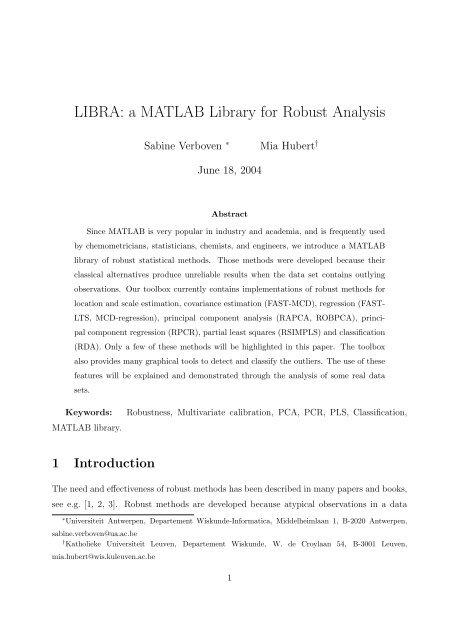
<strong>LIBRA</strong>: a <strong>MATLAB</strong> <strong>Library</strong> <strong>for</strong> <strong>Robust</strong> <strong>Analysis</strong><br />
Sabine Verboven ∗ Mia Hubert †<br />
June 18, 2004<br />
Abstract<br />
Since <strong>MATLAB</strong> is very popular in industry and academia, and is frequently used<br />
by chemometricians, statisticians, chemists, and engineers, we introduce a <strong>MATLAB</strong><br />
library of robust statistical methods. Those methods were developed because their<br />
classical alternatives produce unreliable results when the data set contains outlying<br />
observations. Our toolbox currently contains implementations of robust methods <strong>for</strong><br />
location and scale estimation, covariance estimation (FAST-MCD), regression (FAST-<br />
LTS, MCD-regression), principal component analysis (RAPCA, ROBPCA), princi-<br />
pal component regression (RPCR), partial least squares (RSIMPLS) and classification<br />
(RDA). Only a few of these methods will be highlighted in this paper. The toolbox<br />
also provides many graphical tools to detect and classify the outliers. The use of these<br />
features will be explained and demonstrated through the analysis of some real data<br />
sets.<br />
Keywords: <strong>Robust</strong>ness, Multivariate calibration, PCA, PCR, PLS, Classification,<br />
<strong>MATLAB</strong> library.<br />
1 Introduction<br />
The need and effectiveness of robust methods has been described in many papers and books,<br />
see e.g. [1, 2, 3]. <strong>Robust</strong> methods are developed because atypical observations in a data<br />
∗ Universiteit Antwerpen, Departement Wiskunde-In<strong>for</strong>matica, Middelheimlaan 1, B-2020 Antwerpen,<br />
sabine.verboven@ua.ac.be<br />
† Katholieke Universiteit Leuven, Departement Wiskunde, W. de Croylaan 54, B-3001 Leuven,<br />
mia.hubert@wis.kuleuven.ac.be<br />
1
set heavily affect the classical estimates. Consider <strong>for</strong> example, estimating the center of the<br />
following univariate data set: (10 10.1 10.1 10.1 10.2 10.2 10.3 10.3). For these data, the<br />
classical mean is 10.16 whereas the robust median equals 10.15. They do not differ very<br />
much as there are no outliers. However, if the last measurement was wrongly recorded as<br />
103 instead of 10.3, the mean becomes 21.75 whereas the median still equals 10.15. As in<br />
this example, outliers can occur by mistake (misplacement of a comma), or e.g. through<br />
a malfunction of the machinery or a measurement error. These are typically the samples<br />
that should be discovered and removed from the data unless one is capable to correct their<br />
measurements. Another type of atypical observations are those that belong to another pop-<br />
ulation than the one under study (<strong>for</strong> example, by a change in the experimental conditions)<br />
and often they reveal unique properties. Consequently, finding this kind of outliers can lead<br />
to new discoveries. Outliers are thus not always wrong or bad, although this terminology is<br />
sometimes abusively used.<br />
Over the years, several robust methods became available in SAS [4] and S-PLUS/R [5],<br />
[6]. To make them also accessible <strong>for</strong> <strong>MATLAB</strong> users, we started collecting robust methods<br />
in a <strong>MATLAB</strong> library. The toolbox mainly contains implementations of methods that have<br />
been developed at our research groups at the University of Antwerp and the Katholieke<br />
Universiteit Leuven. It currently contains functions <strong>for</strong> location and scale estimation, co-<br />
variance estimation (FAST-MCD), regression (FAST-LTS, MCD-regression), principal com-<br />
ponent analysis (RAPCA, ROBPCA), principal component regression (RPCR), partial least<br />
squares (RSIMPLS) and classification (RDA).<br />
In this paper we will highlight some methods of the toolbox and apply them to real data<br />
sets. We distinguish between low and high-dimensional data since they require a different<br />
approach. The application of robust methods not only yield estimates which are less in-<br />
fluenced by outliers, they also allow to detect the outlying observations by looking at the<br />
residuals from a robust fit. That’s why we have included in our toolbox many graphical<br />
tools <strong>for</strong> model checking and outlier detection. In particular we will show how to interpret<br />
several diagnostic plots that are developed to visualize and classify the outliers.<br />
In Section 2 a few estimators of location, scale and covariance (including PCA) will be<br />
considered. Some robust regression methods are discussed in Section 3. <strong>Robust</strong> classification<br />
is illustrated in Section 4. Finally, Section 5 contains a list of the currently available main<br />
functions.<br />
2
2 Location, scale and covariance estimators<br />
2.1 Low dimensional estimators<br />
<strong>Robust</strong> estimators of location and scale <strong>for</strong> univariate data include the median, the median<br />
absolute deviation, and M-estimators. In our toolbox we have included several methods<br />
which are described in [7] (and references therein). Also the medcouple, which is a robust<br />
estimator of skewness [8], is available. Here, we will concentrate on the problem of location<br />
and covariance estimation of multivariate data as it is the cornerstone of many multivariate<br />
techniques such as PCA, calibration and classification.<br />
In the multivariate location and scatter setting we assume that the data are stored in an<br />
n × p data matrix X = (x1, . . . , xn) T with xi = (xi1, . . . , xip) T the ith observation. Hence<br />
n stands <strong>for</strong> the number of objects and p <strong>for</strong> the number of variables. In this section we<br />
assume in addition that the data are low-dimensional. Here, this means that p should at<br />
least be smaller than n/2 (or equivalently that n > 2p).<br />
<strong>Robust</strong> estimates of the center µ and the scatter matrix Σ of X can be obtained by the<br />
Minimum Covariance Determinant (MCD) estimator [9]. The MCD method looks <strong>for</strong> the<br />
h(> n/2) observations (out of n) whose classical covariance matrix has the lowest possible<br />
determinant. The raw MCD estimate of location is then the average of these h points,<br />
whereas the raw MCD estimate of scatter is their covariance matrix, multiplied with a<br />
consistency factor. Based on these raw MCD estimates, a reweighting step can be added<br />
which increases the finite-sample efficiency considerably [10].<br />
The MCD estimates can resist (n − h) outliers, hence the number h (or equivalently the<br />
proportion α = h/n) determines the robustness of the estimator. The highest resistance<br />
towards contamination is achieved by taking h = [(n + p + 1)/2]. When a large proportion<br />
of contamination is presumed, h should thus be chosen close to αn with α = 0.5. Otherwise<br />
an intermediate value <strong>for</strong> h, such as 0.75n, is recommended to obtain a higher finite-sample<br />
efficiency. This is also the default setting in our <strong>MATLAB</strong> implementation. It will give<br />
accurate results if the data set contains at most 25% of aberrant values, which is a reasonable<br />
assumption <strong>for</strong> most data sets.<br />
The computation of the MCD estimator is non-trivial and naively requires an exhaustive<br />
investigation of all h-subsets out of n. In [10] a fast algorithm is presented (FAST-MCD)<br />
which avoids such a complete enumeration. It is a resampling algorithm which starts by<br />
3
drawing 500 random p + 1 subsets from the full data set. This number is chosen to ensure a<br />
high probability of sampling at least one clean subset. The mcdcov function in our toolbox is<br />
an implementation of this FAST-MCD algorithm. Note that the MCD can only be computed<br />
if p < h, otherwise the covariance matrix of any h-subset has zero determinant. Since n/2 <<br />
h, we thus require that p < n/2. However, detecting several outliers becomes intrinsically<br />
delicate when n/p is small as some data points may become coplanar by chance. This is an<br />
instance of the “curse of dimensionality”. It is there<strong>for</strong>e recommended that n/p > 5 when<br />
α = 0.5 is used. For small n/p it is preferable to use the MCD with α = 0.75.<br />
With our toolbox the reweighted MCD-estimator of a data set X is computed by typing<br />
>> out=mcdcov(X)<br />
at the command line. Doing so, the user accepts all the default settings: α = 0.75, ‘plots’=1,<br />
‘cor’=0, ‘ntrial’=500. It means that diagnostic plots will be drawn, no correlation matrix<br />
will be computed and the algorithm uses 500 random initial p + 1 subsets.<br />
If the user wants to change one or more of these default settings, the input arguments<br />
and their new values have to be specified. Assume <strong>for</strong> example that we have no idea about<br />
the amount of contamination and we prefer to apply a highly robust method. If in addition,<br />
we are interested in the corresponding MCD correlation matrix, we set:<br />
>> out=mcdcov(X,‘alpha’,0.50,‘cor’,1)<br />
Similar to all <strong>MATLAB</strong> built-in graphical functions, we have chosen to work with variable<br />
input arguments. More precisely, the input arguments in the function header consist of N<br />
required input arguments and a variable range of optional arguments<br />
>> result = functionname(required1,required2,...,requiredN,varargin)<br />
Depending on the application, required input arguments are e.g. the design matrix X, the<br />
response variable y in regression, the group numbers in a classification context etc. The<br />
function call should assign a value to all the required input arguments in the correct order.<br />
However, the optional arguments can be omitted (which implies that the defaults are used)<br />
or they can be called in an arbitrary order. For example,<br />
or<br />
>> out=mcdcov(X,‘cor’,1,‘alpha’,0.50)<br />
4
out=mcdcov(X,‘cor’,1,‘alpha’,0.50,‘plots’,1)<br />
would produce the same result. All our main functions use these user-friendly variable<br />
input arguments. Standard <strong>MATLAB</strong> functions on the other hand (except the graphical<br />
ones) contain all the input arguments in an ordered way such that none of the in-between<br />
arguments can be left out.<br />
The output of mcdcov (and of many other functions in the toolbox) is stored as a struc-<br />
ture. A structure in <strong>MATLAB</strong> is an array variable which can contain fields of different types<br />
and/or dimensions. If a single output variable is assigned to the mcdcov function, the given<br />
solution is the reweighted MCD-estimator. To obtain the results of the raw MCD estimator,<br />
a second output variable has to be assigned<br />
>> [rew,raw]=mcdcov(X)<br />
The structure and content of the output variable(s) is explained in the next example.<br />
Example 1: To illustrate the MCD method we analyze the Stars data set [3]. This is a<br />
bivariate data set (p = 2) where the surface temperature and the light intensity of n = 47<br />
stars were observed. The data were preprocessed by taking a logarithmic trans<strong>for</strong>mation of<br />
both variables. Applying ‘out=mcdcov(X)’ yields the following output structure:<br />
center : [4.4128 4.9335]<br />
cov : [2 × 2 double]<br />
cor : []<br />
h : 36<br />
alpha : 0.7500<br />
md : [1 × 47 double]<br />
rd : [1 × 47 double]<br />
flag : [1 × 47 logical]<br />
cutoff : [1 × 1 struct]<br />
plane : []<br />
method : [1 × 42 char]<br />
class :<br />
′ ′<br />
MCDCOV<br />
classic : 0<br />
X : [47 × 2 double]<br />
5
Here, the output consists of several fields that contain the location estimate (‘out.center’),<br />
the estimated covariance matrix (‘out.cov’) and eventually the correlation matrix (‘out.cor’).<br />
Other fields such as ‘out.h’ and ‘out.alpha’ contain in<strong>for</strong>mation about the MCD method,<br />
while some of the components (e.g. ‘out.rd’, ‘out.flag’, ‘out.md’ and ‘out.cutoff’) can be<br />
used <strong>for</strong> outlier detection and to construct some graphics. The ‘out.class’ field is used by<br />
the makeplot function to detect which figures should be created <strong>for</strong> this analysis. Detailed<br />
in<strong>for</strong>mation about this output structure (and that of the raw estimates) can be found in the<br />
help-file of the mcdcov function.<br />
The robust distance of an observation i is used to detect whether it is an outlier or not.<br />
It is defined as<br />
<br />
RDi =<br />
−1<br />
(xi − ˆµ T<br />
MCD) ˆΣ MCD(xi − ˆµ MCD) (1)<br />
with ˆµ MCD and ˆΣMCD the MCD location and scatter estimates. This robust distance is the<br />
straight<strong>for</strong>ward robustification of the Mahalanobis distance<br />
<br />
MDi =<br />
(xi − ¯x) T S −1 (xi − ¯x) (2)<br />
which uses the classical mean ¯x and empirical covariance matrix S as estimates of location<br />
and scatter. Under the normal assumption, the outliers are those observations having a<br />
<br />
robust distance larger than the cutoff-value χ2 p,0.975, and they receive a flag equal to zero.<br />
<br />
The regular observations whose robust distance does not exceed χ2 p,0.975 have a flag equal<br />
to one.<br />
Based on the robust distances and the Mahalanobis distances, several graphical displays<br />
are provided to visualize the outliers and to compare the robust and the classical results.<br />
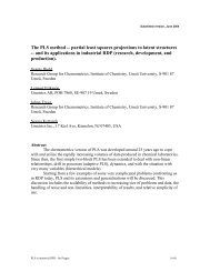
One of them is the distance-distance plot [10] which displays <strong>for</strong> each observation its robust<br />
distance RDi versus its Mahalanobis distance MDi.<br />
<br />
A horizontal and a vertical line are<br />
drawn at the cut-off value χ2 p,0.975. For the stars data, we obtain Figure 1(a) with the<br />
cutoff-lines drawn at 2.72. Looking at Figure 1(a) we clearly see four outlying observations:<br />
11, 20, 30 and 34. Those four observations are known to be giant stars and hence strongly<br />
differ from the other stars in the main sequence. Both a classical and a robust analysis<br />
would identify these observations as they exceed the horizontal and the vertical cut-off line.<br />
Further we observe 3 observations (7, 9, and 14) with a large robust but a small Mahalanobis<br />
distance. They would not be recognized with a classical approach.<br />
As this data set is bivariate, we can understand its structure much better by making a<br />
6
scatter plot as in Figure 1(b). Superimposed is the 97.5% robust confidence ellipse defined as<br />
<br />
the set of points whose robust distance is equal to χ2 p,0.975. Obviously, observations outside<br />
this tolerance ellipse then correspond with the outliers. We again notice the 7 outliers found<br />
with the MCD method.<br />
<strong>Robust</strong> Distance<br />
16<br />
14<br />
12<br />
10<br />
8<br />
6<br />
4<br />
2<br />
9<br />
0<br />
0 0.5 1 1.5 2 2.5 3<br />
Mahalanobis Distance<br />
7<br />
14<br />
11<br />
34<br />
30<br />
20<br />
log(Intensity)<br />
6<br />
5.5<br />
5<br />
4.5<br />
4<br />
3.5<br />
34<br />
30<br />
20<br />
11<br />
Tolerance ellipse ( 97.5 % )<br />
7<br />
3.5 4<br />
log(Temperature)<br />
4.5<br />
(a) (b)<br />
Figure 1: <strong>Analysis</strong> of the Star data set : (a) distance-distance plot ; (b) data with 97.5%<br />
tolerance ellipse.<br />
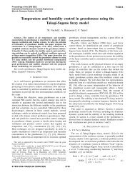
Note that these plots are automatically generated by the mcdcov function. Unless the<br />
input argument ‘plots’ is set to 0, all the main functions call the makeplot function at the<br />
end of the procedure. A small menu with buttons is then displayed, from which the user can<br />
choose one, several, or all available plots associated with the analysis made. For example,<br />
mcdcov offers the menu shown in Figure 2. If the input argument ‘classic’ is also set to<br />
one in the call to the main function, some buttons also yield the figures associated with the<br />
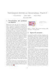
classical analysis. To illustrate, the plots in Figure 3 are the result of computing<br />
>> out=mcdcov(X,’classic’,1)<br />
and pressing the buttons ‘Tolerance ellipse’ and ‘Index plot of the distances’. We see in<br />
Figure 3(a) that the robust and the classical tolerance ellipse are superimposed on the same<br />
plot which is easier <strong>for</strong> comparison. To generate plots, one can also set the input argument<br />
‘plots’ equal to zero, and make a separate call to the makeplot function. In our example, by<br />
typing<br />
>> out=mcdcov(X,’classic’,1,’plots’,0)<br />
>> makeplot(out,’classic’,1)<br />
7<br />
14<br />
9
Figure 2: The graphical user interface invoked by the makeplot function, applied to an<br />
MCDCOV attribute.<br />
log(Intensity)<br />
6.5<br />
6<br />
5.5<br />
5<br />
4.5<br />
4<br />
3.5<br />
34<br />
30<br />
20<br />
robust<br />
classical<br />
Tolerance ellipse (97.5%)<br />
3.4 3.6 3.8 4 4.2 4.4 4.6 4.8 5<br />
log(Temperature)<br />
Mahalanobis distance<br />
3<br />
2.5<br />
2<br />
1.5<br />
1<br />
0.5<br />
MCDCOV<br />
20<br />
0<br />
0 5 10 15 20 25<br />
Index<br />
30 35 40 45<br />
(a) (b)<br />
Figure 3: <strong>Analysis</strong> of the Star data set : (a) data with 97.5% classical and robust tolerance<br />
ellipses; (b) Index plot of the Mahalanobis distances.<br />
The appearance of the graphical menu can be avoided by adding the name of the desired<br />
graph as input argument to the makeplot function. To generate Figure 1 we could e.g. use<br />
the commands<br />
8<br />
30<br />
34
out=mcdcov(X,’plots’,0)<br />
whereas Figure 3 can be created by typing<br />
>> makeplot(out,’nameplot’,’dd’)<br />
>> makeplot(out,’nameplot’,’ellipse’)<br />
>> out=mcdcov(X,’classic’,1,’plots’,0)<br />
>> makeplot(out,’nameplot’,’ellipse’,’classic’,1)<br />
>> makeplot(out,’nameplot’,’mahdist’,’classic’,1)<br />
2.2 High dimensional estimators<br />
If X contains more variables than observations (p ≫ n) its covariance structure can be<br />
estimated by means of a principal component analysis (PCA). In general, PCA constructs<br />
a new set of k ≪ p variables, called loadings, which are linear combinations of the orig-<br />
inal variables and which contain most of the in<strong>for</strong>mation. These loading vectors span a<br />
k-dimensional subspace. Projecting the observations onto this subspace yields the scores ti<br />
which <strong>for</strong> all i = 1, . . . , n satisfy<br />
ti = P T<br />
k,p(xi − ˆµ x) (3)<br />
with the loading matrix P p,k containing the k loading vectors columnwise, and ˆµ x being an<br />
estimate of the center of the data. From here on, the subscripts to a matrix serve to recall<br />
its size, e.g. P p,k is an p × k matrix. In classical PCA these loadings vectors correspond<br />
with the k dominant eigenvectors of S, the empirical covariance matrix of the observations<br />
xi, whereas ˆµ x is just the sample mean. As a byproduct of a PCA analysis, an estimate of<br />
the covariance structure of X can be obtained by the matrix product<br />
ˆΣp,p = P p,kLk,kP T<br />
k,p<br />
with Lk,k a diagonal matrix containing the eigenvalues from the PCA analysis.<br />
A robust PCA method yields robust loadings P , robust eigenvalues L, a robust center<br />
ˆµ x and robust scores according to (3). Our toolbox contains two robust PCA methods. The<br />
first one, called RAPCA [11], is solely based on projection pursuit, and is very fast. The<br />
second method, ROBPCA [12] combines projection pursuit ideas with the MCD estimator<br />
and outper<strong>for</strong>ms RAPCA in many situations. The computation time of ROBPCA is still<br />
9<br />
(4)
very reasonable although slower than RAPCA (e.g. it takes only 4.7 seconds on a Pentium<br />
IV with 2.40 GHz to per<strong>for</strong>m ROBPCA on a data set with n = 30 and p = 2050).<br />
Example 2: We will illustrate ROBPCA and its diagnostic tools on the Octane data set [13]<br />
which consists of n = 39 NIR-spectra of gasoline at p = 251 wavelengths. When we would<br />
know the optimal number of components k, we could call the robpca method with k specified,<br />
e.g.<br />
>> out=robpca(X,’k’,3)<br />
Otherwise, we need to select the number of principal components k. The function call is<br />
then just simply<br />
>> out=robpca(X)<br />
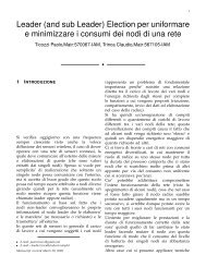
which generates a scree plot. This is a graph of the monotone decreasing eigenvalues. The<br />
optimal number k is then often selected as the one where the kink in the curve appears.<br />
From the scree plot of the Octane data in Figure 4(a), we decide to retain k = 3 components<br />
<strong>for</strong> further analysis. To visualize and to classify the outliers, we can make a (score) outlier<br />
Eigenvalue<br />
10<br />
8<br />
6<br />
4<br />
2<br />
0<br />
x 10 −3<br />
ROBPCA<br />
1 2 3 4 5 6 7 8 9 10<br />
Index<br />
Orthogonal distance<br />
1<br />
0.9<br />
0.8<br />
0.7<br />
0.6<br />
0.5<br />
0.4<br />
0.3<br />
0.2<br />
0.1<br />
29<br />
0<br />
3<br />
(a) (b)<br />
ROBPCA<br />
25<br />
0 10 20 30 40 50 60<br />
Score distance (3 LV)<br />
Figure 4: PC analysis of the Octane data set : (a) Screeplot ; (b) Score diagnostic plot.<br />
map. For each observation, it displays on the x-axis the score distance SDi within the PCA<br />
subspace<br />
SDi =<br />
<br />
t T i L −1 ti<br />
10<br />
37<br />
36<br />
39<br />
38<br />
(5)<br />
26
and on the y-axis the orthogonal distance to the PCA subspace<br />
ODi = ||xi − ˆµ x − P p,kti||. (6)<br />
This yields a classification of the observations as summarized in Table 1: regular data (with<br />
small SD and small OD), good PCA-leverage points (with large SD and small OD), orthogo-<br />
nal outliers (with small SD and large OD) and bad PCA-leverage points (with large SD and<br />
large OD). The latter two types of observations are highly influential <strong>for</strong> classical PCA as<br />
this method tries to make all orthogonal distances as small as possible. For more in<strong>for</strong>mation<br />
on this outlier map and the horizontal and vertical cut-off values, we refer to Reference [12].<br />
On the outlier map of the Octane data in Figure 4(b) we immediately spot the samples 25,<br />
26, 36-39 as bad PCA-leverage points. It is known that these samples contain added alcohol,<br />
hence their spectra are indeed different from the other spectra. This becomes very clear<br />
from the outlier map.<br />
Table 1: Overview of the different types of observations based on their score distance and<br />
their orthogonal distance.<br />
Distances small SD large SD<br />
large OD orthogonal outlier bad PCA-leverage point<br />
small OD regular observation good PCA-leverage point<br />
3 <strong>Robust</strong> calibration<br />
3.1 Low dimensional regressors<br />
The multiple linear regression model assumes that in addition to the p regressors or x-<br />
variables, a response variable y is measured, which can be explained as an affine combination<br />
of the predictors. More precisely, the model says that <strong>for</strong> all observations (xi, yi) with<br />
i = 1, . . . , n, it holds that<br />
yi = β0 + β1xi1 + · · · + βpxip + ɛi = β0 + β T xi + ɛi i = 1, . . . , n (7)<br />
where the errors ɛi are assumed to be independent and identically distributed with zero mean<br />
and constant variance σ2 . Applying a regression estimator to the data yields p +1 regression<br />
coefficients ˆθ = ( ˆ β0, . . . , ˆ βp). The residual ri of case i is defined as yi − ˆyi = yi − ˆθ T<br />
xi.<br />
11
The ordinary least squares (OLS) estimator minimizes the sum of the squared residuals,<br />
but is very sensitive to outliers. Our toolbox contains the Least Trimmed Squares (LTS)<br />
estimator [9] which minimizes the sum of the h smallest squared residuals, or<br />
ˆθLTS = min<br />
θ<br />
h<br />
i=1<br />
(r 2 )i:n<br />
Note that the residuals are first squared, and then ordered. The interpretation of the h value<br />
is the same as <strong>for</strong> the MCD estimator, and should be chosen between n/2 and n. Taking h =<br />
n yields the OLS estimator. The <strong>MATLAB</strong> function ltsregres contains an implementation<br />
of the FAST-LTS algorithm [14] which is similar to the FAST-MCD method. The output<br />
of ltsregres includes many graphical tools <strong>for</strong> model checking and outlier detection, such<br />
as a normal quantile plot of the residuals, and a residual outlier map. The latter displays<br />
the standardized LTS residuals (the residuals divided by a robust estimate of their scale)<br />
versus the robust distances obtained by applying the MCD estimator on the x-variables. Its<br />
interpretation will be discussed in Section 3.2.<br />
If we want a reliable prediction of q > 1 properties at once, based on a set of p explanatory<br />
variables, the use of a multivariate regression method is appropriate. The linear regression<br />
model is then <strong>for</strong>mulated as<br />
y i = β 0 + B T xi + εi i = 1, . . . , n (9)<br />
with y i and εi being q-dimensional vectors that contain the response values, respectively the<br />
error terms of the ith observation with covariance matrix Σε.<br />
To cope with such data, we can use the MCD-regression method [15, 16]. It is based on<br />
the MCD estimates of the joint (x, y) variables and thereby yields a highly robust method.<br />
Within our toolbox, this method can be called with the mcdregres function.<br />
3.2 High dimensional regressors<br />
In case the number of variables p is larger than the number of observations n, there is no<br />
unique OLS solution, and neither can the LTS estimator be computed. Moreover, in any data<br />
set with highly correlated variables, called multicollinearity, both OLS and LTS have a high<br />
variance. Two very popular solutions to this problem are offered by Principal Component<br />
Regression (PCR) and Partial Least Squares Regression (PLSR). Both methods first project<br />
12<br />
(8)
the x-data onto a lower dimensional space without loosing too much important in<strong>for</strong>mation.<br />
Then a multiple or multivariate regression analysis is per<strong>for</strong>med in this lower dimensional<br />
design space.<br />
More precisely, both PCR and PLSR assume the following bilinear model which expresses<br />
the connection between the response variable(s) and the explanatory variables as:<br />
with ti the k-dimensional scores, k ≪ p and q ≥ 1.<br />
xi = µ x + P p,kti + f i (10)<br />
y i = µ y + Aq,kti + g i (11)<br />
To construct the scores ti, PCR applies PCA to the x-variables, whereas in PLSR they<br />
are constructed by maximizing the covariance between linear combinations of the x and<br />
y-variables. <strong>Robust</strong> versions of PCR and PLSR have been constructed in [16] and [17] with<br />
corresponding <strong>MATLAB</strong> functions rpcr and rsimpls. In analogy with classical PCR and<br />
PLSR, they apply ROBPCA on the x-variables, respectively the joint (x, y) variables. Next,<br />
a robust regression is applied to model (11). For PCR we can use the LTS or the MCD<br />
regression, whereas <strong>for</strong> PLSR a regression based on the ROBPCA results is per<strong>for</strong>med.<br />
Example 2 continued: Let us look again at the Octane data from Section 2.2. The<br />
univariate (q = 1) response variable contains the octane number. We know from the previous<br />
analysis that in samples 25,26,36-39 alcohol was added. We cannot use an ordinary least<br />
squares regression since the data clearly suffers from multicollinearity, so we apply a robust<br />
PCR analysis. We then first need to determine the optimal number of components k. To this<br />
end, the robust cross-validated RMSE can be computed at the model with k = 1, . . . , kmax<br />
components. For a <strong>for</strong>mal definition, see [16]. This is a rather time-consuming approach,<br />
but faster methods <strong>for</strong> its computation have been developed and will become part of the<br />
toolbox [18]. Alternatively, a robust R 2 -plot can be made. To look at the RMSECV-curve,<br />
the function call in <strong>MATLAB</strong> becomes:<br />
>> out=rpcr(X,y,’rmsecv’,1)<br />
Here, the robust RMSECV-curve in Figure 5(a) shows k = 3 as the optimal number of latent<br />
variables (LV).<br />
The output of the rpcr function also includes the score and orthogonal distances from the<br />
robust PCA analysis. So by default the PCA-outlier map will again be plotted (Figure 4b).<br />
13
R−RMSECV value<br />
0.8<br />
0.7<br />
0.6<br />
0.5<br />
0.4<br />
0.3<br />
0.2<br />
0.1<br />
1 2 3 4 5 6 7 8 9 10<br />
Number of components<br />
Standardized residual<br />
4<br />
3<br />
2<br />
1<br />
0<br />
−1<br />
−2<br />
−3<br />
−4<br />
7<br />
13<br />
0 10 20 30 40 50 60<br />
Score distance (3 LV)<br />
(a) (b)<br />
Figure 5: <strong>Analysis</strong> of the Octane data set : (a) <strong>Robust</strong> RMSECV-curve; (b) Regression<br />
outlier map.<br />
Table 2: Overview of the different types of observations based on their score distance and<br />
their absolute residual.<br />
Distances small SD large SD<br />
RPCR<br />
large absolute residual vertical outlier bad leverage point<br />
small absolute residual regular observation good leverage point<br />
In addition, a residual outlier map is generated. It displays the standardized LTS residuals<br />
versus the score distances, and can be used to classify the observations according to the<br />
regression model. As can be seen from Table 2, we distinguish regular data (small SD and<br />
small absolute residual), good leverage points (large SD but small absolute residual), vertical<br />
outliers (small SD and large absolute residual), and bad leverage points (large SD and large<br />
<br />
absolute residuals). Large absolute residuals are those that exceed χ2 1,0.975 = 2.24. Under<br />
normally distributed errors, this happens with probability 2.5%. The vertical outliers and<br />
bad leverage points are the most harmful <strong>for</strong> classical calibration methods as they disturb<br />
the linear relationship.<br />
Note that the observations that are labeled on the outlier map are by default the three<br />
cases with the largest score distance, and those three that have the largest absolute stan-<br />
dardized residual. To change these settings, one should assign different values to the ‘labod’,<br />
14<br />
25<br />
37<br />
39<br />
36<br />
38<br />
26
‘labsd’ and ‘labrd’ input arguments. For example, Figure 5(b) was the result of<br />
>> makeplot(out,’labsd’,6,’labrd’,2)<br />
In multivariate calibration (q > 1) the residuals are also q-dimensional with estimated co-<br />
variance matrix ˆ Σε. The outlier map then displays on the vertical axis the residual distances,<br />
defined as<br />
with cut-off value<br />
<br />
χ 2 q,0.975.<br />
4 Classification<br />
ResDi =<br />
<br />
r T i ˆ Σ −1<br />
ε ri<br />
Classification is concerned with separating different groups. Classification rules or discrimi-<br />
nant rules aim at finding boundaries between several populations, which then allow to classify<br />
new samples. We assume that our data are split into m different groups, with nj observations<br />
in group j (and n = <br />
j nj). The Bayes discriminant rule classifies an observation to<br />
the group j <strong>for</strong> which the discriminant score d Q<br />
j (x) is maximal, with<br />
d Q<br />
j (x) = −1<br />
2 ln|Σj| − 1<br />
2 (x − µ j) T Σ −1<br />
j (x − µ j) + ln(pj). (12)<br />
Here, µ j and Σj are the center and (non-singular) covariance matrix of the jth population,<br />
and pj is its membership (or prior) probability. The resulting discriminant rule is quadratic in<br />
x, from which the terminology ’quadratic discriminant analysis’ is derived. If the covariance<br />
structure of all groups is equal, or Σj = Σ, the discriminant scores reduce to<br />
which is linear in x.<br />
d L j (x) = µ T j Σ −1 x − 1<br />
2 µT j Σ −1 µ j + ln(pj) (13)<br />
Classical classification uses the group means and covariances in (12) and (13), whereas the<br />
membership probabilities are often estimated as nj/n. In robust discriminant analysis [19]<br />
the MCD estimates of location and scatter of each group are substituted in (12). For the<br />
linear case, we can use the pooled MCD scatter estimates as an estimate <strong>for</strong> the overall Σ.<br />
Finally, the membership probabilities can be robustly estimated as the relative frequency<br />
of regular observations in each group, which are those whose flag resulting from the MCD<br />
procedure is equal to one.<br />
15
One also needs a tool to evaluate a classification rule, i.e. we need an estimate of the as-<br />
sociated probability of misclassification. Our <strong>MATLAB</strong> function contains three procedures.<br />
The apparent probability of misclassification counts the (relative) frequencies of badly classi-<br />
fied observations from the training set. But it is well known that this yields a too optimistic<br />
estimate as the same observations are used to determine and to evaluate the discriminant<br />
rule. With the cross-validation approach the classification rule is constructed by leaving out<br />
one observation at a time and then one sees whether this observation is correctly classified or<br />
not. Because it makes little sense to evaluate the discriminant rule on outlying observations,<br />
one could apply this procedure by leaving out the non-outliers one by one, and counting the<br />
percentage of badly classified ones. This approach is rather time-consuming, especially at<br />
larger data sets, but approximate methods can be used [18] and will become available in the<br />
toolbox. As a third and fast approach, the proportion of misclassified observations from the<br />
validation set can be computed. Because it can happen that this validation set also contains<br />
outlying observations which should not be taken into account, we estimate the misclassifi-<br />
cation probability MPj of group j by the proportion of non-outliers from the validation set<br />
that belong to group j and that are badly classified.<br />
Example 3: The Fruit data set analyzed in [19] was obtained by personal communication<br />
with Colin Greensill (Faculty of Engineering and Physical Systems, Central Queensland<br />
University, Rockhampton, Australia) and resumed here. The original data set consists of<br />
2818 spectra measured at 256 wavelengths. It contains 6 different cultivars of a cantaloupe.<br />
We proceed in the same way as in [19] where only 3 cultivars (D, M, and HA) were considered,<br />
leaving 1096 spectra. Next a robust principal component analysis was applied to reduce the<br />
dimension of the data. It would be dangerous to apply classical PCA here as the first<br />
components could be highly attracted by possible outliers and would not give a good low-<br />
dimensional representation of the data. (Also in [20] it was illustrated that preprocessing<br />
high dimensional spectra with a robust PCA method resulted in a better classification.) For<br />
illustrative purposes two components were retained and a linear discriminant analysis was<br />
per<strong>for</strong>med. To per<strong>for</strong>m the classification, the data were randomly split up into a training set<br />
and a validation set, consisting of 60% resp. 40% of the observations. It was told that the<br />
third cultivar HA consists of 3 groups obtained with different illumination systems. However,<br />
the subgroups were treated as a whole since it was not clear whether they would behave<br />
16
differently. Given this in<strong>for</strong>mation the optional input argument ’alpha’ which measures the<br />
fraction of outliers the MCD-algorithm should resist, was set to 0.5. The <strong>MATLAB</strong> call to<br />
rda additionally includes the training set X, the corresponding vector with group numbers<br />
g, the validation set Xtest and its group labels gtest, and the method used (’linear’ or<br />
’quadratic’):<br />
>> out=rda(X,g,’valid’,Xtest,’groupvalid’,gtest,’alpha’,0.5,’method’,’linear’)<br />
For the fruit data, we obtain ˆpD = 51%, ˆpM = 13% and ˆpHA = 36% whereas the misclas-<br />
sification probabilities were 16% in cultivar D, 95% in cultivar M, and 6% in cultivar HA.<br />
Cultivar M’s high misclassification probability is due to its overlap with the other groups<br />
and because of its rather small number of samples (nM = 106) in contrast to the other 2<br />
groups (nD = 490 and nHA = 500). The misclassification probability of HA on the other<br />
hand is very small because its estimate does not take into account the outlying data points.<br />
In Figure 6 a large group of outliers is spotted on the right side. The 97.5% tolerance el-<br />
lipses are clearly not affected by that group of anomalous data points. In fact, the outlying<br />
group coincides with a subgroup of the cultivar HA which was caused by the change in the<br />
illumination system.<br />
Component 2<br />
4<br />
3<br />
2<br />
1<br />
0<br />
−1<br />
D<br />
M<br />
HA<br />
−2<br />
−10 −5 0 5 10 15 20<br />
Component 1<br />
Figure 6: <strong>Analysis</strong> of the Fruit data set: 97.5% robust tolerance ellipses <strong>for</strong> each cultivar<br />
obtained from a linear discriminant rule.<br />
Note that when data are high-dimensional, the approach of this section can not be applied<br />
anymore because the MCD becomes uncomputable. In the example of the fruit data, this was<br />
solved by applying a dimension reduction procedure (PCA) on the whole set of observations.<br />
17
Instead, one can also apply a PCA method on each group separately. This is the idea behind<br />
the SIMCA method (Soft Independent Modeling of Class Analogy) [21]. A robust variant of<br />
SIMCA can be obtained by applying a robust PCA method, such as ROBPCA (Section 2.2),<br />
within each group. This approach is currently under development [22].<br />
5 Availability and outlook<br />
<strong>LIBRA</strong>, the <strong>MATLAB</strong> library <strong>for</strong> <strong>Robust</strong> <strong>Analysis</strong>, can be downloaded from one of the<br />
following web sites:<br />
http://www.wis.kuleuven.ac.be/stat/robust.html<br />
http://www.agoras.ua.ac.be/<br />
These programs are provided free <strong>for</strong> non-commercial use only. They can be used with<br />
<strong>MATLAB</strong> 5.2, 6.1 and 6.5. Some of the functions require the <strong>MATLAB</strong> Statistics toolbox.<br />
The main functions currently included in the toolbox are listed in Table ??. In the near<br />
future, we will add implementations of fast methods <strong>for</strong> cross-validation [18], S-estimators of<br />
location and covariance [23], S-estimators of regression [24], the LTS-subspace estimator [25],<br />
an adjusted boxplot <strong>for</strong> skewed distributions [26], and robust SIMCA [22].<br />
Acknowledgments<br />
We acknowledge (in alphabetical order) Guy Brys, Sanne Engelen, Peter Rousseeuw, Nele<br />
Smets, Karlien Vanden Branden, and Katrien Van Driessen <strong>for</strong> their important contributions<br />
to the toolbox.<br />
References<br />
[1] P.J. Huber, <strong>Robust</strong> Statistics, Wiley: New York, 1981.<br />
[2] F.R. Hampel, E.M. Ronchetti, P.J. Rousseeuw, W.A. Stahel, <strong>Robust</strong> Statistics: The<br />
Approach Based on Influence Functions, Wiley: New York, 1986.<br />
[3] P.J. Rousseeuw, A. Leroy, <strong>Robust</strong> Regression and Outlier Detection, John Wiley: New<br />
York, 1987.<br />
18
[4] C. Chen, <strong>Robust</strong> Regression and Outlier Detection with the ROBUSTREG Procedure in<br />
Proceedings of the Twenty-Seventh Annual SAS Users Group International Conference,<br />
SAS Institute Inc, Cary, NC, 2002.<br />
[5] A. Marazzi, Algorithms, Routines and S Functions <strong>for</strong> <strong>Robust</strong> Statistics, Belmont:<br />
Wadsworth, 1993.<br />
[6] S-PLUS 6 <strong>Robust</strong> <strong>Library</strong> User’s Guide, Insightfull Corporation, Seattle, WA.<br />
[7] P.J. Rousseeuw, S. Verboven, Comput. Statist. Data Anal. 40 (2002) 741 – 758.<br />
[8] G. Brys, M. Hubert, A. Struyf, J. Comput. Graph. Statist., in press, available at<br />
http://www.wis.kuleuven.ac.be/stat/robust.html.<br />
[9] P.J. Rousseeuw, J. Amer. Statist. Assoc. 79 (1984) 891 – 880.<br />
[10] P.J. Rousseeuw, K. Van Driessen, Technometrics 41 (1999) 212 – 223.<br />
[11] M. Hubert, P.J. Rousseeuw, S. Verboven, Chemom. Intell. Lab. Syst. 60 (2002) 101 –<br />
111.<br />
[12] M. Hubert, P.J. Rousseeuw, K. Vanden Branden, Technometrics, in press, available at<br />
http://www.wis.kuleuven.ac.be/stat/robust.html.<br />
[13] K.H. Esbensen, Multivariate Data <strong>Analysis</strong> in Practice, Camo Process AS (5th edition),<br />
2001.<br />
[14] P.J. Rousseeuw, K. Van Driessen, in W. Gaul, O. Opitz, and M. Schader (Eds.), Data<br />
<strong>Analysis</strong>: Scientific Modeling and Practical Application, Springer-Verlag, New York,<br />
2000, pp. 335 – 346.<br />
[15] P.J. Rousseeuw, S. Van Aelst, K. Van Driessen, A. Agullo, Technometrics, in press,<br />
available at http://www.agoras.ua.ac.be.<br />
[16] M. Hubert, S. Verboven, J. Chemom. 17 (2003) 438 – 452.<br />
[17] M. Hubert, K. Vanden Branden, J. Chemom. 17 (2003) 537 – 549.<br />
[18] S. Engelen, M. Hubert, Fast cross-validation in robust PCA, COMPSTAT 2004 Pro-<br />
ceedings, edited by J. Antoch, Springer, Physica-Verlag.<br />
19
[19] M. Hubert, K. Van Driessen, Comput. Statist. Data Anal. 45 (2004) 301 – 320.<br />
[20] M. Hubert, S. Engelen, Bioin<strong>for</strong>matics, 20 (2004), 1728-1736.<br />
[21] S. Wold, Pattern Recognition 8 (1976) 127 – 139.<br />
[22] K. Vanden Branden, M. Hubert, <strong>Robust</strong> classification of high-dimensional data, COMP-<br />
STAT 2004 Proceedings, edited by J. Antoch, Springer, Physica-Verlag.<br />
[23] L. Davies, Ann. Statist. 15 (1987) 1269–1292.<br />
[24] P.J. Rousseeuw, V.J. Yohai, in J. Franke, W. Härdle and R.D. Martin (Eds.), <strong>Robust</strong><br />
and Nonlinear Time Series <strong>Analysis</strong>, Lecture Notes in Statistics No. 26. Springer-Verlag:<br />
New York, 1984, pp. 256 – 272.<br />
[25] S. Engelen, M. Hubert, K. Vanden Branden, A comparison of three procedures <strong>for</strong><br />
robust PCA in high dimensions, Proceedings of CDAM2004, BSU Publishing House.<br />
[26] E. Vandervieren, M. Hubert, An adjusted boxplot <strong>for</strong> skewed distributions, COMPSTAT<br />
2004 Proceedings, edited by J. Antoch, Springer, Physica-Verlag.<br />
20
Function Description<br />
<strong>Robust</strong> estimators of location/scale/skewness<br />
mlochuber M-estimator of location, with Huber psi-function.<br />
mloclogist M-estimator of location, with logistic psi-function.<br />
hl Hodges-Lehmann location estimator.<br />
unimcd MCD estimator of location and scale.<br />
mad Median absolute deviation with finite sample correction factor (scale).<br />
mscalelogist M-estimator of scale, with logistic psi-function.<br />
qn Qn-estimator of scale.<br />
adm Average distance to the median (scale).<br />
mc Medcouple, a robust estimator of skewness.<br />
<strong>Robust</strong> multivariate analysis<br />
l1median L1 median of multivariate location.<br />
mcdcov Minimum Covariance Determinant estimator of multivariate location<br />
and covariance.<br />
rapca <strong>Robust</strong> principal component analysis (based on projection pursuit).<br />
robpca <strong>Robust</strong> principal component analysis (based on projection pursuit<br />
and MCD estimation).<br />
rda <strong>Robust</strong> linear and quadratic discriminant analysis.<br />
robstd Columnwise robust standardization.<br />
<strong>Robust</strong> regression methods<br />
ltsregres Least Trimmed Squares regression.<br />
mcdregres Multivariate MCD regression.<br />
rpcr <strong>Robust</strong> principal component regression.<br />
rsimpls <strong>Robust</strong> partial least squares regression.<br />
Plot functions<br />
makeplot creates plots <strong>for</strong> the main statistical functions (including residual plots<br />
and outlier maps).<br />
normqqplot normal Quantile-Quantile plot.<br />
Classical multivariate analysis and regression<br />
ols Ordinary (multiple linear) least squares regression.<br />
classSVD Singular value decomposition if n > p.<br />
kernelEVD Singular value decomposition if n < p.<br />
cpca Classical principal component analysis.<br />
mlr Multiple linear regression (with one or several response variables).<br />
cpcr Classical principal component regression.<br />
csimpls Partial least squares regression (SIMPLS).<br />
cda Classical linear and quadratic discriminant analysis.<br />
Table 3: List of the current main functions in <strong>LIBRA</strong>, the <strong>MATLAB</strong> <strong>Library</strong> <strong>for</strong> <strong>Robust</strong><br />
<strong>Analysis</strong>. 21