Universe
Universe
Universe

You also want an ePaper? Increase the reach of your titles
YUMPU automatically turns print PDFs into web optimized ePapers that Google loves.
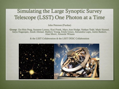
Simulating the Large Synoptic Survey<br />
Telescope (LSST) One Photon at a Time<br />
John Peterson (Purdue)<br />
Group: En-Hsin Peng, Suzanne Lorenz, Kari Frank, Mary Ann Hodge, Nathan Todd, Mark Hannel,<br />
Satya Nagarajan, Zarah Ahmad, Mallory Young, Emily Grace, Alexandra Lupu, Justin Bankert,<br />
Alan Meert, Amanda Winans<br />
& the LSST Collaboration & the LSST DESC Collaboration
Most measurements<br />
have suggested a<br />
<strong>Universe</strong> of mostly dark<br />
energy, some dark<br />
matter, and little baryon<br />
filled <strong>Universe</strong><br />
CMB ~ total content:<br />
few % within critical<br />
Clusters ~ DM/atoms<br />
ratio is ~6<br />
Supernovae~DE<br />
dominant in expansion<br />
BBN ~ small fraction of<br />
atoms<br />
Modern Cosmology<br />
Dark<br />
Matter<br />
22%<br />
Atoms<br />
4%<br />
Dark<br />
Energy<br />
74%<br />
Is this even right? 96% of the <strong>Universe</strong> is beyond<br />
the Standard Model. What is the consequence of<br />
this? What can we measure about these further?
Future Measurements in Cosmology<br />
Need more data to get higher statistical precision<br />
Need multiple astrophysical techniques<br />
However, when you push towards higher statistical<br />
precision have new systematics that need to be<br />
understood<br />
And with a large enough quantity of data & high<br />
enough precision would need both fast and high<br />
fidelity simulations to understand these details
High Precision Cosmological Techniques<br />
1) SNe to Measure Expansion Rate<br />
(Perlmutter 1998; Reiss 1998)<br />
2) Time delays in strong lens images<br />
(Suyu 2010)<br />
3) Cluster Mass Function Evolution<br />
(Vikhlinin 2009; JRP 2012)<br />
Growth of Structure (e.g. Springel 2005)<br />
4) Baryon<br />
Acoustic<br />
Oscillations in<br />
Matter Power<br />
Spectrum<br />
(Eisenstein 2005)
5) Weak Gravitational Lensing<br />
High Precision Cosmological Techniques<br />
Knox et. al 2004
High Precision Cosmological Techniques<br />
Hu 2008<br />
Dark Energy Constraints<br />
Will have increasing<br />
discriminatory power<br />
to distinguish between<br />
cosmological constant<br />
and various models<br />
LSST will measure:<br />
3 billion galaxies<br />
10 billion stars<br />
1 million SNe<br />
10,000 clusters<br />
Dark Matter Map<br />
of Entire Sky<br />
[Also the other major area requiring high precision is stellar astrometry where large<br />
Fraction of milky way will be mapped with proper motions & some parallaxes]
How does LSST do this? Etendue<br />
Etendue is the product of<br />
Area and Field of View<br />
To get more area simply build<br />
a large telescope<br />
To get higher field of view, favor<br />
designs with shorter focal lengths,<br />
and minimal vignetting, reasonable<br />
off-axis image quality<br />
Consequence of this is have to<br />
build a large camera<br />
Consequence of a large camera is<br />
large data rate
Large Synoptic Survey Telescope (LSST)<br />
Adler Planetarium, Brookhaven National Laboratory (BNL), California Institute<br />
of Technology, Carnegie Mellon University, Chile, Cornell University, Drexel<br />
University, Fermi National Accelerator Laboratory, George Mason University,<br />
Google, Inc., Harvard-Smithsonian Center for Astrophysics, Institut de Physique<br />
Nucleaire et de Physique des Particules (IN2P3), Johns Hopkins University,<br />
Stanford University, Las Cumbres Observatory Global Telescope Network, Inc.,<br />
Lawrence Livermore National Laboratory (LLNL), Los Alamos National<br />
Laboratory (LANL), National Optical Astronomy Observatory, Princeton<br />
University, Purdue University, Research Corporation for Science Advancement,<br />
Rutgers University, SLAC National Accelerator Laboratory, Space Telescope<br />
Science Institute, Texas A & M University, The Pennsylvania State University,<br />
University of Arizona, University of California at Davis, University of California<br />
at Irvine, University of Illinois at Urbana-Champaign, University of Michigan,<br />
University of Pennsylvania, University of Pittsburgh, University of Washington,<br />
Vanderbilt University<br />
Largest survey telescope: Highest Etendue (area*FOV)<br />
for a telescope: 320 m2deg2 www.lsst.org<br />
Largest data rate 10Tb/night!<br />
8.4 m mirror; 6 filters (300-1100 nm)<br />
Largest Astronomical Camera<br />
Joint NSF & DoE project<br />
Commissioning in ~2019;<br />
First science observations in ~2021<br />
Surveys the ½ the sky every few nights<br />
Get ~1000 images in 6 colors over 10 years to ~27 mag<br />
of everything (billions of galaxies & stars, & all<br />
asteroids >150 m, rare objects)
LSST Site
LSST Mirrors
LSST Camera
Importance of Simulations for LSST<br />
More data than any other astronomical project<br />
Produces 3 gigapixel images (~1500 HDTV’s) every 15<br />
seconds<br />
No one can ever look at all the data Automatic<br />
processing (that has to work when telescope turns on)<br />
In addition, some of the most accurate measurements ever<br />
made have been planned especially for cosmology<br />
Maybe we should do some simulations<br />
Have led development of a novel photon simulation<br />
(phoSim) code for several years in the LSST project
COSMO-<br />
LOGICAL<br />
SIMULATOR:<br />
Synthetic<br />
<strong>Universe</strong> is<br />
constructed<br />
DESC Simulation & Analysis Framework<br />
object 0.002 -<br />
2.439485 14.5<br />
galaxySED/Const64e<br />
0804z..spec.gz 0 0 0<br />
0 0 0 sersic2D<br />
1.29394 2.4587 1.77<br />
2.980 ccm 2.3 8.2<br />
ccm 2.78 9.45<br />
<strong>Universe</strong> Catalogs Photons Images <br />
Measurements<br />
CATALOG<br />
CONSTRUCTOR<br />
(CATSIM):<br />
<strong>Universe</strong> is<br />
parameterized<br />
in catalogs that<br />
can later be<br />
photon sampled<br />
PHOTON SIMULATOR<br />
(PHOSIM):<br />
Atmosphere,<br />
Telescope, &<br />
Camera physics<br />
formulated in terms<br />
of photon<br />
manipulations<br />
Image Simulations (IMSIM)=PHOSIM+CATSIM<br />
w=-1.00000<br />
+/- 0.00001<br />
DATA<br />
MANAGEMENT (DM) &<br />
DESC LEVEL-3<br />
ANALYSIS:<br />
Image processing to<br />
produce catalogs and<br />
measurements<br />
on the catalogs<br />
14
First order image properties<br />
Photometric zeropoint<br />
Background level<br />
PSF size<br />
Astrometric scale<br />
Image Properties<br />
Some existing simulators (Sky Maker (Bertin),<br />
Shapelets (Dobke), GalFast (Mandelbaum),<br />
DES (Lin)) use parametric models to capture<br />
some image properties<br />
To get detailed second image properties have<br />
to go to full photon Monte Carlo approach<br />
Essentially all DE measurements depend on<br />
some combination of detailed PSF<br />
size/shape, astrometry, or photometry<br />
Second Order Image properties<br />
PSF size wavelength dependence<br />
PSF size spatial dependence<br />
PSF size spatial variation<br />
PSF shape (ellipticity and other moments)<br />
PSF wings<br />
PSF shape wavelength-dependence<br />
PSF shape spatial decorrelation<br />
PSF shape spatial variation<br />
Differential astrometric non-linearity<br />
Differential astrometric wavelength-dependence<br />
Differential astrometric decorrelation<br />
Photometric chromaticity<br />
Photometric variation in time<br />
Background spatial dependence<br />
Background spatial variation<br />
Background wavelength dependence<br />
And more…
Optical Photon Monte Carlo Simulations
Sky:<br />
Observing configuration from OpSim<br />
Photon Monte Carlo for Galaxies (elliptical Sersic<br />
bulge/disk), Stars, Asteroids (moves during & between<br />
exposures)<br />
Dust absorption at source & Milky Way<br />
Separate SEDs for every object<br />
Instance Catalogs to include other objects<br />
Background of blank sky, moon, twilight, inc. gradients<br />
Atmosphere:<br />
Multi-layer multi-scale frozen Kolmogorov screens<br />
Outer scale model<br />
Seasonal Wind model for LSST site<br />
Turbulence vs. height model for LSST site<br />
Atmospheric raytrace (refractive turbulence & optical<br />
depth)<br />
Atmospheric dispersion<br />
Atmospheric molecular opacity (wavelength, height, &<br />
time dependent)<br />
Multi-level grey cloud model<br />
Physics of PhoSim<br />
Optics & Detector:<br />
Reflection/Refraction in optics/detector<br />
Diffraction<br />
LSST Optics Design (filter-dependent)<br />
Focal plane layout<br />
Two-level Spider design<br />
Alt/Az Tracking Errors, Rotation Jitter, Spider rotation<br />
Dome Seeing<br />
Surface Perturbations & Alignment errors of<br />
mirrors/lenses/detectors<br />
Large Angle Scattering<br />
Angle-dependent filter curves<br />
Lens coatings<br />
Mirror Reflectivity<br />
Saturation & Blooming<br />
Detector A/R<br />
QE & Charge diffusion model<br />
Cosmic rays<br />
Read Noise, Dark Current, Gain, Pre-scans, Offsets<br />
for amplifiers<br />
Hot pixels/columns & dead pixels<br />
Non-uniform QE Maps<br />
CTE<br />
Biases/Darks/Flats<br />
Complete Optimization for saturation, background, photon removal,<br />
& non-sequential rays<br />
17
Very important physics<br />
PSF size, shape, & astrometry (where the photon lands)<br />
Optical Design<br />
Perturbations/Misalignments<br />
Charge Diffusion<br />
Turbulence<br />
Photometry (how many photons)<br />
Geometric design<br />
Rayleigh scattering<br />
Filter multi-layer coatings<br />
Photo-electric conversion<br />
18
Regimes of<br />
Image Simulation<br />
Aberrations+Diffusion<br />
>> λ(f/#)<br />
Aberrations+Diffusion<br />
r 0~10 cm<br />
D > r 0~ 10cm<br />
D D/v ~ .1s<br />
Modern Survey Telescopes
Monte Carlo Efficiency<br />
Basically doing a Monte Carlo over the incident radiation field through<br />
Time-dependent & Wavelength-dependent Physics<br />
Extremely fast way of doing this integral even if we have large numbers of photons
PhoSim<br />
Architecture<br />
Static Physics & Design Data<br />
SEDs of <strong>Universe</strong>,<br />
sky background/moon data<br />
LSST camera, telescope, &<br />
site specific files<br />
Cosmic ray templates,<br />
Earth-specific atmosphere data<br />
Code<br />
Data<br />
User<br />
User<br />
Integration<br />
Validation<br />
Tests<br />
Loop over visits<br />
Instance Catalog<br />
Operation<br />
Commands<br />
Astro<br />
Catalog<br />
Physics<br />
command<br />
override files<br />
(optional)<br />
Loop over chips<br />
Trim<br />
PhoSim<br />
script<br />
Photon<br />
Raytrace<br />
Instrument<br />
Config<br />
Extra Outputs:<br />
eimage<br />
Centroid files<br />
Surface throughput<br />
files<br />
Event files<br />
Atmosphere<br />
Creator<br />
Electron<br />
->ADC<br />
Loop over<br />
exposures<br />
Amplifier<br />
images
Catalog Constructor<br />
Connolly, Krughoff, Gibson (UW)<br />
A catalog of positions, motions (proper motions, orbits), and<br />
physical properties (types, SEDs, spatial model, etc.) of<br />
objects expected to be seen by LSST.<br />
It is a multi-billion row relational database, and a suite of<br />
Python tools.<br />
Used to create “instance catalogs” what is in the sky at<br />
a given time and what are their spatial & spectral properties;<br />
Include operational data of environment and observation<br />
control (moon position, filter, exposure, etc.)<br />
LSST Operation Simulator
Galaxies from ΛCDM N-Body Simulations: Galaxy positions and properties from<br />
Millennium N-body simulation catalogs with gas cooling, star formation,<br />
supernovae and AGN (Lucia et al. 2008); Up to 28 mag in r-band/23 million galaxies<br />
Morphologies modeled with combination of Sérsic profiles – ellipticals and bulge +<br />
disk (Lucia et al., Gonzalez et al.); Spectral Energy Distribution fit to colors of source using<br />
spectral models (Bruzual & Charlot)<br />
Milky Way model of 10 million detectable stars; Based on state-of-the-art Galactic<br />
structure models surveys (Juric et al. (2008), Ivezic et al. (2008), Bond et al. (2010), Sesar, Juric and Ivezic<br />
(2011), Lopez-Corredoira et al. (2005)); Includes a full three-dimensional Interstellar dust<br />
distribution model to redden SEDs of stars & galaxies (Amores & Lepine (2005), matched to<br />
Schlegel, Finkbeiner, Davis (1998) maps at infinity)<br />
10.6 M object Solar System Model w/ orbits & obs. Properties: inclues Near Earth<br />
Objects,Main Belt Asteroids, Trojans, Trans-Neptunian Objects, Scattered Disk<br />
Objects, (PanSTARRS Model, PASP 123, 423 (2011),Bottke et al 2002, Morbidelli et al, Grav et al. 2011)<br />
Variable stars and transient objects (e.g. SNe)<br />
r-i (mag)<br />
CatSim<br />
g-r (mag) g-r (mag)<br />
SDSS
Draw Photons<br />
Direction: Direction chosen by (ra, dec) and telescope pointing<br />
(ra,dec) & rotator angle<br />
Wavelength: Monte Carlo Sample SED files to choose<br />
wavelength in rest frame of source<br />
Time: Monte Carlo Sample time between start and stop of<br />
exposure<br />
Position: Start at the top of the atmosphere in pupil pattern<br />
Additional Astrophysics:<br />
Redshift: photon has wavelength redshifted after drawing from rest frame<br />
Dust: Two dust models that destroy the photons according to reddening laws; Apply both in<br />
the rest frame for internal reddening & in our frame from Milky Way models<br />
Lensing: Extended source models can be distorted by measuring their position from the center<br />
of the source and distorting final position of photon according to γ1 and γ2 24
Kolmogorov~k -11/3<br />
r 0<br />
Outer Scale<br />
Aperture size<br />
Atmosphere Turbulence<br />
Phase screens<br />
Temperature fluctuation in the<br />
atmosphere cause index of refraction<br />
variations and result in “seeing”<br />
Well-known that atmospheric<br />
turbulence has approximately<br />
Kolmogorov spectrum (k -11/3 ) up to<br />
outer scale L 0 (von Karman)<br />
These patterns are essentially frozen<br />
and drift with constant velocity in a<br />
series of layers (Taylor)
Atmosphere Model<br />
Photons accumulate<br />
Refractive kicks through<br />
Frozen drifted phase screens<br />
of turbulence;<br />
Possibly lost due to opacity<br />
Diffraction on scales below 2 r 0<br />
treated by full diffraction calculation<br />
Atmospheric Dispersion simulated
Atmosphere Structure<br />
Wind model (direction & data) uses data<br />
based on seasonal monthly averages for<br />
LSST latitude and longitude<br />
Model for turbulence intensity as a<br />
Function of height<br />
Model for outer scale a function of height
Atmosphere Opacity<br />
1) Cloud model<br />
2) Molecular opacity<br />
O 3<br />
O 2<br />
H 2O<br />
3) Rayleigh scattering<br />
4) Aerosols<br />
Have complex spatial & temporal variation<br />
Local optical depth calculated for each ray<br />
segment<br />
Absorption is pressure-dependent and therefore<br />
height dependent
Star Grids<br />
29
Raytracing through<br />
Telescope & Camera Optics<br />
Series of optical surfaces (2D)<br />
that divide the 3-D volume into<br />
different media (glass, silicon, air)<br />
Ray intercepts are found by<br />
minimizing the distance between the<br />
end of the ray and the surface<br />
Interactions can occur at interfaces<br />
(reflection, refraction, absorption)
Each filter configuration has every surface<br />
defined by the asphere equation<br />
Each surface specifies the media (silicon, glass, air) between the surface<br />
in the 3-D volume<br />
Chips in detector plane specified by rectangular surfaces having a<br />
nominal center, pixel size, x & y sizes<br />
Name Type R curv Δz r out r in κ α 3 α 4<br />
Optical Elements<br />
α 5<br />
α 6<br />
α 7<br />
α 8<br />
α 9<br />
α 10<br />
Coating Medium<br />
M1 Mirror 19835 0 4180 2558 -1.215 0 0 0 1.381e-27 0 0 0 0 Mirror Vacuum<br />
M2 Mirror 6788 6156.2 1710 900 -0.222 0 0 0 -1.274e-23 0 -9.68e-<br />
31<br />
M3 Mirror 8344.5 -6390 2508 550 0.155 0 0 0 -4.5e-25 0 -8.15e-<br />
33<br />
0 0 Mirror Vacuum<br />
0 0 Mirror Vacuum<br />
None None 0 3630.5 0 0 0 0 0 0 0 0 0 0 0 None Vacuum<br />
L1 Lens 2824 34.568418 775 0 0 0 0 0 0 0 0 0 0 Lens A/R Glass<br />
L1E Lens 5021 82.23 775 0 0 0 0 0 0 0 0 0 0 Lens A/R Vacuum<br />
L2 Lens 0 412.64202 551 0 0 0 0 0 0 0 0 0 Lens A/R Glass<br />
L2E lens 2529 30 551 0 -1.57 0 0 1.656e-21 0 0 0 0 Lens A/R Vacuum<br />
F filter 5632 349.58 378 0 0 0 0 0 0 0 0 0 Filter 0 Glass<br />
FE filter 5530 26.60 378 0 0 0 0 0 0 0 0 0 None Vacuum<br />
L3 lens 3169 42.40 361 0 -0.962 0 0 0 0 0 0 0 Lens A/R Glass<br />
L3E lens -13360 60 361 0 0 0 0 0 0 0 0 0 Lens A/R Vacuum<br />
31
Every optical surface & CCD has an ideal location<br />
Perturbations,<br />
Misalignments,<br />
& Tracking Errors<br />
During a particular simulation all surfaces & CCDs can be misaligned by the 6<br />
degrees of freedom; Each optical surface can also have a surface perturbations<br />
place on the surface that represent the deviation from the ideal shape<br />
These represent the perturbations & misalignments induced by the thermal,<br />
vibrational, pressure, gravitational stresses while the telescope is operating with<br />
the full control system as well as fabrication errors<br />
In general, the perturbations & misalignments tend to induce anisotropic PSFs<br />
that are highly correlated across the entire focal plane (because mostly in pupil<br />
plane)<br />
Also have tracking model for perturbations during an exposure<br />
dxi = fiu ¥ + dxi dT T -T ( 0 +dTgT ) + dxi dq q +dqg ( m)<br />
+ hig0 + Aij ( aj +da jga )<br />
-1 -1<br />
aj = Aji Pi + Ajl Zlk<br />
æ<br />
ç<br />
è<br />
-1 ak ç<br />
1+<br />
Navg ö<br />
g ÷<br />
0 ÷<br />
ø<br />
ZkiUi
Multilayer Coatings<br />
Photons reflected or transmitted<br />
according to multilayer models<br />
which are angle and wavelength<br />
dependent<br />
Photoelectron Conversion<br />
Photons can convert into electrons<br />
as they traverse the Silicon<br />
(temperature-dependent)
After 1 micron<br />
After 10 microns<br />
Rasmussen<br />
After 100 microns<br />
After 50 microns After 300 microns<br />
Electron Diffusion<br />
First, electric field profile as a function of<br />
height is calculated (voltage & dopant density<br />
model dependent)<br />
Then electron is drifted in segments and lateral<br />
diffusion is set by local diffusion constant;<br />
Leads to non-gaussian profile
Other Effects<br />
Spider diffraction<br />
Dome seeing<br />
Large angle scattering from mirror<br />
micro-roughness & Mie scattering<br />
Bleeding & Saturation<br />
Ghosts<br />
Cosmic Rays
Background Model<br />
Two components:<br />
Air glow & scattered<br />
Moonlight<br />
Moon has Mie scattering &<br />
Rayleigh scattering which<br />
leads to color-dependent<br />
spatial gradient<br />
Airglow has spatial<br />
variation & temporal<br />
variation<br />
Adams et al.
Digitization<br />
Amplifier Segmentation<br />
CTE (one electron at a time)<br />
Pre/Over scans<br />
ADC using bias, gain, nonlinearity<br />
model with variation<br />
Bit error in ADC<br />
Dark current<br />
Read noise & variation<br />
Hot pixels<br />
Hot columns<br />
Dead Pixels<br />
PRNU
0.2”<br />
Optics +Tracking +Diffraction +Det Perturbations<br />
+Lens Perturbations +Mirror Perturbations +Detector +Dome Seeing<br />
+Low Altitude +Mid Altitude +High Altitude +Pixelization<br />
Atmosphere Atmosphere Atmosphere<br />
38
0.2”<br />
Optics +Tracking +Diffraction +Det Perturbations<br />
+Lens Perturbations +Mirror Perturbations +Detector +Dome Seeing<br />
+Low Altitude +Mid Altitude +High Altitude +Pixelization<br />
Atmosphere Atmosphere Atmosphere 39
Entire<br />
focal plane<br />
3<br />
gigapixels<br />
1000 CPU<br />
hours<br />
1 trillion<br />
photons<br />
Done on<br />
grid<br />
computing
Central<br />
5 x 5 chips<br />
~1 sq. degree<br />
41
Central chip<br />
15’ x 15’<br />
42
ImSim Description 44
ImSim Description 45
3 Color<br />
Image
4 Major LSST Data Challenges so far (4/09,6/10,9/10,5/11,4/12); Run on grid computing at Purdue<br />
(incl. OSG), UW, SLAC, and Google; Currently produce data at ~10% of real time; All analyzed by<br />
Data Management Pipelines<br />
4 thousand visits<br />
28 million amplifier images<br />
44 billion astrophysical objects<br />
4 quadrillion photons<br />
Photometry<br />
Everything<br />
compared to<br />
simulation truth<br />
(not possible<br />
with real data)<br />
Astrometry Completeness PSF size & shape
JRP, Bard, Allen, Li, Cui<br />
Blind shear survey with 10 sq. degrees<br />
Estimated shear systematic floor<br />
Chang et al. 2012
Validation!
Conclusions<br />
Have a multi-purpose high fidelity optical image<br />
simulator (PhoSim) with physics appropriate for<br />
optical survey telescopes<br />
Will enable a number of state-of-the art algorithms to<br />
be developed that necessary for high precision<br />
cosmological measurements in the LSST DESC<br />
LSST will enable dark energy properties to be<br />
measured in unprecented detail & will make dark<br />
matter map of the entire sky<br />
Also possible to use for other telescopes