GPU algorithms for comparison-based sorting and for merging ...

GPU algorithms for comparison-based
sorting and for merging based on
multiway selection
Diplomarbeit
von
Nikolaj Leischner
am Institut für Theoretische Informatik, Algorithmik II
der Fakultät für Informatik
Erstgutachter: Prof. Dr. rer. nat. Peter Sanders
Zweitgutachter: Prof. Dr. rer. nat. Dorothea Wagner
Betreuender Mitarbeiter: M.Sc. Vitaly Osipov
Bearbeitungszeit: 2. Februar 2010 – 29. Juli 2010

Ich erkläre hiermit, dass ich die vorliegende Arbeit eigenhändig angefertigt habe und
keine anderen als die angegebenen Hilfsmittel verwendet habe.
(Nikolaj Leischner)
2

Special thanks go to Sebastian Bauer and Olaf Liebe for helpful discussions, and for
enduring my endless rantings about the painful debugging of GPU programs. Further
thanks go to my supervisor Vitaly Osipov, foremost for supporting my work and also for
giving me motivation when I needed it.
4

Contents
1 Abstract (German) 7
2 Introduction 9
2.1 Motivation . . . . . . . . . . . . . . . . . . . . . . . . . . . . . . . . . . . 9
2.2 Thesis structure . . . . . . . . . . . . . . . . . . . . . . . . . . . . . . . . 10
2.3 Work methodology . . . . . . . . . . . . . . . . . . . . . . . . . . . . . . 10
3 Basics 11
3.1 GPU architectures . . . . . . . . . . . . . . . . . . . . . . . . . . . . . . 11
3.2 GPU programming languages . . . . . . . . . . . . . . . . . . . . . . . . 12
3.3 Performance analysis and modeling for GPU algorithms . . . . . . . . . . 13
3.4 Parallel primitives . . . . . . . . . . . . . . . . . . . . . . . . . . . . . . . 14
3.5 Programming methodologies for GPUs . . . . . . . . . . . . . . . . . . . 14
3.5.1 SIMD-conscious vs. SIMD-oblivious algorithm design . . . . . . . 14
3.5.2 Multiprocessor-conscious vs. -oblivious algorithm design . . . . . 15
4 Related work 15
4.1 Basic strategies for parallel sorting . . . . . . . . . . . . . . . . . . . . . 15
4.2 Sorting and merging on GPUs . . . . . . . . . . . . . . . . . . . . . . . . 16
4.3 Sorting on multi-core CPUs . . . . . . . . . . . . . . . . . . . . . . . . . 17
5 GPU merging 17
5.1 Algorithm overview . . . . . . . . . . . . . . . . . . . . . . . . . . . . . . 17
5.2 Multiway selection (multi sequence selection) . . . . . . . . . . . . . . . . 18
5.2.1 Sequential multi sequence selection . . . . . . . . . . . . . . . . . 19
5.2.2 Parallel multi sequence quick select . . . . . . . . . . . . . . . . . 22
5.3 Parallel merging . . . . . . . . . . . . . . . . . . . . . . . . . . . . . . . . 24
5.3.1 Comparator networks . . . . . . . . . . . . . . . . . . . . . . . . . 24
5.3.2 Odd-even and bitonic merge . . . . . . . . . . . . . . . . . . . . . 25
5.3.3 Parallel ranking . . . . . . . . . . . . . . . . . . . . . . . . . . . . 26
5.3.4 Block-wise merging . . . . . . . . . . . . . . . . . . . . . . . . . . 26
5.3.5 Pipelined merging . . . . . . . . . . . . . . . . . . . . . . . . . . . 28
5.3.6 Other parallel merging approaches . . . . . . . . . . . . . . . . . 29
5.4 Sorting by merging . . . . . . . . . . . . . . . . . . . . . . . . . . . . . . 30
5.5 Experimental results . . . . . . . . . . . . . . . . . . . . . . . . . . . . . 30
5.5.1 Hardware setup . . . . . . . . . . . . . . . . . . . . . . . . . . . . 30
5.5.2 Input data . . . . . . . . . . . . . . . . . . . . . . . . . . . . . . . 30
5.5.3 Multi sequence selection . . . . . . . . . . . . . . . . . . . . . . . 31
5.5.4 Merging networks . . . . . . . . . . . . . . . . . . . . . . . . . . . 33
5.5.5 Merging . . . . . . . . . . . . . . . . . . . . . . . . . . . . . . . . 34
5.5.6 Sorting . . . . . . . . . . . . . . . . . . . . . . . . . . . . . . . . . 36
5

6 Revisiting GPU Sample sort 37
6.1 Algorithm overview . . . . . . . . . . . . . . . . . . . . . . . . . . . . . . 37
6.2 Algorithm implementation . . . . . . . . . . . . . . . . . . . . . . . . . . 39
6.3 Exploring bottlenecks . . . . . . . . . . . . . . . . . . . . . . . . . . . . . 41
6.3.1 Sorting networks . . . . . . . . . . . . . . . . . . . . . . . . . . . 41
6.3.2 Second level sorting . . . . . . . . . . . . . . . . . . . . . . . . . . 42
6.3.3 k-way distribution . . . . . . . . . . . . . . . . . . . . . . . . . . 42
6.4 GPU Sample Sort vs. revised GPU Sample Sort . . . . . . . . . . . . . . 45
6.5 Other possible implementation strategies . . . . . . . . . . . . . . . . . . 47
7 Converting from Cuda to OpenCL 47
7.1 The OpenCL programming language . . . . . . . . . . . . . . . . . . . . 48
7.2 An OpenCL implementation of GPU Sample Sort . . . . . . . . . . . . . 48
8 Conclusion 50
A Proof of correctness for sequential multi sequence selection 52
A.1 Correctness . . . . . . . . . . . . . . . . . . . . . . . . . . . . . . . . . . 52
A.2 Consistency and stability . . . . . . . . . . . . . . . . . . . . . . . . . . . 53
B Proof of correctness for block-wise merging 54
C CREW PRAM Quicksort 55
6

1 Abstract (German)
Sortieren und Mischen sind zwei grundlegende Operationen, die in zahlreichen Algorithmen
– deren Laufzeit von ihrer Effizienz abhängt – verwendet werden. Für Datenbanken
sind Sortier- und Misch-Algorithmen wichtige Bausteine. Suchmaschinen, Algorithmen
aus der Bioinformatik, Echtzeitgrafik und geografische Informationssysteme stellen weitere
Anwendungsfelder dar. Zudem ergeben sich bei der Arbeit an Sortierroutinen interessante
Muster die sich auf andere algorithmische Probleme übertragen lassen.
Aufgrund der Entwicklungen in der Rechnerarchitektur in Richtung paralleler Prozessoren
stellen parallele Sortier- und Misch-Algorithmen ein besonders relevantes Problem
dar. Es wurden zahlreiche Strategien entwickelt um mit unterschiedlichen Arten von
Prozessoren effizient zu sortieren und zu mischen. Trotzdem gibt es nach wie vor Lücken
zwischen Theorie und Praxis; beispielsweise ist Coles Sortieralgorithmus trotz optimaler
Arbeits- und Schrittkomplexität praktisch langsamer als Algorithmen mit schlechterer
asymptotischer Komplexität. Für Sortiernetzwerke die bereits vor 1970 entdeckt wurden
hat bis heute niemand einen besseren Ersatz gefunden. Sortier- und Misch-Algorithmen
lassen sich auf endlos viele Weisen zu Misch- und Sortier-Strategien kombinieren. Aus
diesen Gründen bleiben Sortieren und Mischen, sowohl aus praktischer, als auch aus
theoretischer Sicht, ein fruchtbares Forschungsgebiet.
Frei programmierbare Grafikprozessoren (GPUs) sind weit verbreitet und bieten ein
sehr gutes Verhältnis von Kosten und Energieverbrauch zu Rechenleistung. GPUs beherbergen
mehrere SIMD-Prozessoren. Ein SIMD-Prozessor (single instruction multiple
data) führt eine Instruktion gleichzeitig für mehrere Datenelemente durch. Mit diesem
Prinzip lassen sich auf auf einem Chip mehr Rechenwerke pro Fläche unterbringen als
bei einem skalaren Prozessor. Jedoch arbeitet ein SIMD-Prozessor nur dann effizient,
wenn es hinreichend viel gleichförmige parallele Arbeit gibt. Zusätzlich verwenden die
Prozessoren einer GPU SMT (simultaneous multi threading); sie bearbeiten mehrere Instruktionen
gleichzeitig um Ausführungs- und Speicherlatenzen zu verdecken. Aus diesen
Eigenschaften ergibt sich dass GPUs nur mit massiv parallelen Algorithmen effizient arbeiten
können.
In dieser Diplomarbeit beschäftigen wir uns mit GPU-Algorithmen für Sortieren und
Mischen. Wir untersuchen eine Parallelisierungsstrategie für die Misch-Operation die bis
dato nur für Multi-core CPUs eingesetzt wurde: Selektion in mehreren sortierten Folgen
(multiway selection, auch bezeichnet als multi sequence selection). Für dieses Problem
stellen wir einen neuen Algorithmus vor und implementieren diesen sowie einen zweiten,
bereits bekannten, Algorithmus für GPUs. Unser neuer Selektionsalgorithmus ist im
Kontext einer Misch-Operation auf GPUs praktikabel, obwohl er nicht massiv parallel
ist. Wir untersuchen verschiedene Techniken um Mischen feingranular zu parallelisieren:
Misch-Netzwerke, sowie hybride Algorithmen, welche Misch-Netzwerke in eine sequentielle
Misch-Prozedur einbinden. Die hybriden Algorithmen bewahren die asymptotische
Komplexität ihrer sequentiellen Gegenstücke und einer von ihnen ist auch der erste
Mehrweg-Misch-Algorithmus für GPUs. Wir zeigen empirisch dass Mehrweg-Mischen
auf aktuellen GPUs keinen Performance-Vorteil gegenüber Zweiweg-Mischen erzielt –
Speicherbandbreite ist beim Sortieren mit GPUs noch kein Flaschenhals. Unser bester
Misch-Algorithmus, der auf Zweiweg-Mischen basiert, zeigt ein 35% besseres Laufzeitverhalten
als vorher veröffentlichte GPU-Implementierungen der Misch-Operation.
7

Weiterhin setzen wir Optimierungen für unseren zuvor veröffentlichten GPU-Sortierer
GPU Sample Sort um und erzielen im Schnitt eine 25% bessere Leistung, in einzelnen
Fällen bis zu 55%. Unsere Implementierung verwenden wir zuletzt als Fallstudie um die
Portierbarkeit von Cuda-Programmen in die Sprache OpenCL zu evaluieren. Während
Cuda lediglich führ GPUs von Nvidia verfügbar ist existieren OpenCL-Implementierungen
auch für GPUs und CPUs von AMD, IBM CELL, und Intels Knights Ferry (Larrabee).
Wir benutzen Nvidias OpenCL-Implementierung um gleichzeitig feststellen zu können
ob es praktikabel ist ganz auf Cuda zu verzichten. Aufgrund von instabilen OpenCL-
Treibern für aktuelle Nvidia-Hardware füren wir den Vergleich nur auf älterern Nvidia-
GPUs durch. Unsere OpenCL-Portierung erzielt dort 88,7% der Leistung unserer Cuda-
Implementierung.
Diese Arbeit stellt einen weiteren Schritt in der Erforschung von Sortieralgorithmen
und Misch-Algorithmen für datenparallele Rechnerarchitekturen dar. Wir untersuchen
alternative Strategien für paralleles Mischen und liefern Bausteine für zukünftige Sortier-
Algorithmen und Mehrweg-Misch-Algorithmen. Der in dieser Arbeit vorgestellte Algorithmus
für Selektion in mehreren sortierten Folgen ist auch für CPUs geeignet. Unsere
Fallstudie zur Portierbarkeit von Cuda nach OpenCL von GPU Sample Sort bietet einen
Anhaltspunkt zur Wahl der Implementierungssprache für GPU-Algorithmen.
8

2 Introduction
2.1 Motivation
Sorting and merging are two important kernels which are used as subroutines in numerous
algorithms, whose performance depends on the efficiency of these primitives. Databases
use sort and merge primitives extensively. Computational biology, search engines, realtime
rendering and geographical information systems are other fields where sorting and
merging large amounts of data is indispensable. Even when their great practical importance
is taken aside; many interesting patterns arise in the design and engineering of
sorting procedures, which can be applied to other types of algorithms [23].
More specifically, parallel sorting is a pervasive topic. Both sorting and merging
are problems that lend themselves to parallelization. Numerous strategies have been
designed that map sorting successfully to different kinds of processor architectures. Yet
there are gaps between theory and practice. Coles parallel merge sort [11], for example,
has optimal work complexity and step complexity. In practice, however, it is so far not
competitive to simpler but theoretically worse algorithms [30]. Sorting networks have
been researched since the 1960s [5]. While networks with lower asymptotic complexity
are known [3], the 40 years old odd-even network and bitonic network are still in use today
because they perform better in practice. Different sorting algorithms can be combined
in countless ways into different sorting strategies. This makes parallel sorting a fruitful
area for research from both a theoretical and practical point of view.
Changes in processor architecture over the last years further motivate the design of
practical parallel algorithms. As the clock rate and performance of sequential processors
starts hitting a wall, the trend has become to put more and more processors on a single
chip. Multi-core CPUs are commonplace already and a shift to many-core CPUs is
likely. Memory bandwidth is not expected to increase in the same manner as parallel
processing power, effectively making memory access more expensive in comparison to
computation and causing processor designers to introduce deeper memory hierarchies.
Current generation GPUs already realize these trends. They also provide computational
power at a favorable cost and power-efficiency. This makes them an ideal playground for
designing and engineering parallel algorithms.
The work on GPU sorting is extensive, see Section 4. However, merging on GPUs
has to our best knowledge thus far only been considered as a sub-step of sorting routines
and as a method for list intersection [13]. In the first part of this thesis we investigate
dedicated merging primitives for GPUs.
Previous GPU merging algorithms either use a recursive merging strategy, or divide
the work with a distribution step, similar to sample sort. We wondered if multiway
selection was a viable strategy for merging on GPUs. Multiway selection (also termed
multi sequence selection) splits a set of sorted sequences into multiple parts of equal size
that can be merged independently. It has previously been employed by multi-core CPU
merge sort algorithms. Its main advantage is that it achieves perfect load balancing for
the subsequent merge step – an important consideration for algorithms on many-core
architectures.
We demonstrate a new multi sequence selection algorithm that is also suitable for
multi-core CPUs and give a proof of correctness for it. We implement the algorithm for
9

GPUs, alongside a different multi sequence selection algorithm. We implement several
strategies to expose fine-grained parallelism in merging: bitonic merging, odd-even merging
and hybrid strategies that combine sequential two-way and four-way merging with
merging networks. The hybrid algorithms maintain asymptotic work efficiency while still
making use of data-parallelism. Our merging primitive achieves a higher performance
than earlier published merging primitives do. A sort based on our merger proves to be
worse than our previously published GPU Sample Sort [25] and worse than a different
recent merge sort implementation [35].
That we cannot match the performance of GPU Sample Sort with our merge sort
motivates the second part of the thesis: we reconsider our implementation of GPU Sample
Sort and improve it incrementally. Our overhauled implementation achieves on average
25% higher performance and up to 55% higher performance for inputs on which our
original implementation performs worst.
At the time of writing most researchers choose Cuda for implementing their GPU algorithms.
Cuda, however, only supports Nvidia GPUs. Conducting experiments on other
hardware platforms like AMD GPUs, Intels upcoming many-core chips or CELL would
increase the validity of experimental results. More important, algorithm implementations
are of greater practical use when they run on more hardware platforms. OpenCL
is supported on AMD GPUs, AMD CPUs, CELL and also available for Nvidia GPUs.
We evaluate the current state of Nvidias OpenCL implementation by implementing GPU
Sample Sort in OpenCL. Due to a lack of stable OpenCL drivers for recent Nvidia GPUs
we are only able to compare an OpenCL implementation to a Cuda implementation on
an older Nvidia GPU (G80). With slight code adjustments we are able to reach 88.7% of
our Cuda implementations performance.
2.2 Thesis structure
This thesis is divided into 8 sections. The first two lay out the motivation for our work
and include a short summary. Section 3 introduces the basic concepts of GPU architectures
and GPU programming. A discussion of related work follows in Section 4. In
Section 5 we discuss the components of our GPU merging routines and provide an extensive
experimental analysis. Our previous work [25] is shortly revisited in Section 6.
We then explore the bottlenecks of our sample sort algorithm and evaluate an OpenCL
implementation of it in Section 7. Lastly, in Section 8, we summarize our results and
elaborate on possible future work.
2.3 Work methodology
We follow the paradigm of algorithm engineering, which is akin to the process by which
natural science develops novel theories. Instead of taking a linear path from theoretical
design to implementation we interleave design and implementation. While complexity
theory guides our algorithmic choices, we always implement our algorithms and set up
experiments to verify or falsify our choices.
The strong reliance on experiments is motivated by the large gap between theoretical
machine models and actual processor architectures. GPUs exhibit properties of both
SIMD and SPMD architectures, use bulk-synchronous communication and have a deep
10

memory hierarchy. While many of the architectural details are vital for performance, it
is very difficult to fit all of them into a single theoretical model. Thus, experimentation
is mandatory when arguing for an algorithms performance.
3 Basics
In this section we describe the most important properties of the processor architectures
for which our algorithms are designed. Further, basic concepts and terms for parallel
(GPU) algorithms are introduced. In the following, we use the term GPU as a synonym
for stream processor and many-core processor.
3.1 GPU architectures
GPUs differ significantly from traditional general purpose processors. While the latter
are designed to process a sequential stream of arbitrary mixed instructions efficiently,
GPUs excel at solving computationally intense data-parallel problems. A GPU consists
of several SIMD processing units (also called multiprocessors). Each SIMD unit consists
of several ALUs, load/store units, a register file and an additional local memory.
Pipelining is used to increase instruction throughput, although in a way that is very different
from that used by CPUs; a multiprocessor executes several SIMD groups in parallel
(SMT). Therefore it can keep its pipeline filled with instructions that are guaranteed to
be independent of each other. This kind of multi-threading has two major implications:
• Branch prediction heuristics, speculative execution, instruction re-ordering and
other complex features used in monolithic scalar processors are less important or
superfluous.
• Caches are rather employed to save bandwidth than to reduce memory access latencies,
since these latencies are already hidden by SMT.
A GPU is connected to a DRAM memory, which, at the time of writing, typically
has a size of several GiBs, and which has more than 100 GB/s bandwidth. Access to
this memory is expensive: the available bandwidth is shared among tens of processors,
and despite multi-threading the high access latencies can only be hidden if there is a
sufficient amount of computation per memory access. For the G200-based Nvidia Tesla
c1060 the instruction throughput is 312 · 10 9 instructions per second, while the memory
throughput is 25.5·10 9 32 bit words per second. Consequently, 12.2 compute instructions
per memory instruction are required on this device to rule out bandwidth limitation.
For the Fermi-based Gigabyte Geforce GTX480 the instruction throughput is 676 · 10 9
instructions per second, and its memory throughput is 44.3 · 10 9 32 bit words per second.
On this device 15.3 compute instructions per memory instruction are required to rule out
bandwidth limitation.
Another property of the GPU off-chip memory is that its transaction size is similar to
that of a CPU cache line. This means that memory access with large strides or unordered
access patterns can reduce the effective bandwidth to a fraction of the peak bandwidth.
The most recent GPUs at the time of writing (Nvidia Fermi and AMD RV870) have two
11

levels of cache for the off-chip memory, which make partially unordered access patterns
less expensive. We refer to the GPUs DRAM as global memory.
To give a clearer picture, we enumerate the most important concrete architectural
parameters of current generation GPUs:
• 14 - 30 multiprocessors for a combined number of 128 - 1600 ALUs per chip.
• A SIMD width of 32 or 64 and SMT of 2 - 48 SIMD groups per multiprocessor.
• Register files of size 1024 × 32 bit per multiprocessor, up to 16384 × 128 bit per
multiprocessor.
• Local shared memory of 16 KiB - 48 KiB per multiprocessor.
• Up to 16 KiB L1 cache per multiprocessor and up to 768 KiB global L2 cache.
• Global memory transaction size of 128 byte.
Analyzing the properties of such complex processor architectures is an interesting
topic in itself. We refer to the work of Wong et al. [39] for an in-depth analysis of
the Nvidia G200 chip (Geforce GTX280, Tesla c1060), which is our primary development
platform for this work – although we carry out most of our final benchmarks on a Geforce
GTX480, which is based on the Nvidia Fermi chip.
GPU
Global Memory
DRAM DRAM DRAM DRAM DRAM DRAM DRAM DRAM
Figure 1: Nvidia G200 architecture.
3.2 GPU programming languages
Multiprocessor
SP
SP
SP
SP
SP
SP
Local Memory
Currently, two languages are predominant in GPU programming: Nvidias proprietary
Cuda [1], and OpenCL [2] from the Khronos Group consortium. Cuda runs exclusively
on Nvidia GPUs while OpenCL is also available for AMD GPUs, AMD CPUs and the
CELL processor. Both languages introduce identical abstractions at two levels.
SIMD execution: The slots of an SIMD instruction are mapped to threads. If one is
only concerned by program correctness, then the SIMD property of the hardware
can be ignored. As long as there are only small divergences in the execution paths
of different threads this is even practical – threads of a SIMD group that must
12
SP
SP

not execute an instruction are masked out (branch predication). For greater divergences
the different paths occurring within an SIMD group have to be serialized.
Consequently, processor utilization is reduced by a large degree. Each thread has
a private memory which maps to multiprocessor registers. Communication among
threads takes place through the local memory of the multiprocessor, which is shared
among all threads and which can be synchronized via barrier synchronization.
Pipelining: Each thread belongs to a thread block (OpenCL uses the term work group).
The size of a thread block can and should be greater than the SIMD width of the
hardware. If thread blocks are chosen large enough, then the pipelining properties
of GPUs with differing SIMD widths can be hidden.
Processor virtualization: In addition to the abstractions at the multiprocessor level,
the multiprocessors themselves are also virtualized. Depending on register space,
shared local memory space and scheduling constraints each multiprocessor is able
to execute several thread blocks simultaneously. Further, a GPU program may
consist of a much larger number of thread blocks than can be executed concurrently
by the GPU. The GPUs runtime environment re-schedules thread blocks until all
have finished executing. Therefore a program – given it runs a sufficiently large
number of thread blocks – will run efficiently, regardless of the actual number
of multiprocessors present on a specific GPU. Thread blocks share access to the
DRAM of the GPU. In contrast to the threads of a single block it is impossible
to synchronize threads belonging to different thread blocks during the execution of
a program. Instead, synchronization takes place implicitly when a GPU program
(also called kernel) terminates.
Cudas and OpenCLs abstract machine model can be summarized as a set of uniform
CREW PRAMs with small private memories, barrier synchronization and a large shared
memory to which all PRAMs have access. The machine is programmed in the SPMD
(single program multiple data) paradigm. PRAM indices and thread indices are used to
break the symmetry of a program.
3.3 Performance analysis and modeling for GPU algorithms
In a parallel execution model there are two metrics for measuring the complexity of an
algorithm: the number of time steps for a given problem size, and the total amount of
work required for a given problem size. At the level of individual SIMD groups it is mostly
the step complexity that matters, unless conflicts in memory access lead to serialization.
When looking at thread blocks or the whole set of thread blocks of a GPU algorithm we
are rather interested in modeling the work complexity. The amount of thread blocks and
SIMD groups executed in parallel is typically lower than the total number of thread blocks
of a kernel. Conflicting access to both local multiprocessor memory and global DRAM
incurs further serialization. Therefore, it would be very difficult to model a realistic
step complexity for a GPU algorithm. That said, algorithms with non-optimal work
complexity but superior theoretical step complexity may be more efficient in practice; we
determine this by experimenting.
13

In some places we provide instruction count numbers for our algorithms. We count
arithmetic instructions, assignments, comparisons, synchronizations and branches. This
way of counting is slightly simplified in that we do not differentiate between local memory
and registers – variables from local memory may be transparently cached in registers. Our
estimates are consequently too optimistic.
3.4 Parallel primitives
Our algorithms use two parallel primitives in multiple places: reduction and scan.
Reduction Be an associative operator that can be evaluated in constant time. Compute
i

empty. The downside to SIMD-conscious programming is that algorithms become more
complicated and hardware-specific. When working without explicit synchronization subtle
errors can be introduced. E.g. when diverging execution paths within an SIMD
group are serialized and the implementations behavior unintentionally depends on the
order in which these paths are executed. SIMD-conscious programming is unnecessary if
synchronization barriers are infrequent and threads have a uniform workload. Oblivious
algorithms are more desirable since they tend to be less hardware-specific and easier to
implement. Nevertheless, to use GPUs efficiently, being conscious of SIMD execution is
at times unavoidable.
3.5.2 Multiprocessor-conscious vs. -oblivious algorithm design
Because processors are virtualized, the actual number of multiprocessors present on a
GPU can be ignored in algorithm design and implementation. When parallelization introduces
a significant overhead one strives to split a task among as few thread blocks
as possible. It is then more efficient to launch just enough thread blocks to saturate
a given GPU than to use very many thread blocks. The downside to this approach is
that it might lead to hardware-specific design choices; a strategy might work efficiently
on the GPUs it was developed and tested on but break down on other architectures.
For example when significantly more thread blocks are required to saturate these architectures.
Another practical concern is that it is difficult to determine optimal launch
parameters at run-time without making queries for device names or similar. The Cuda
API provides some functionality for this – multiprocessor count, register file size and
other parameters are known at run-time. Although the device information available in
Cuda is more extensive than it is for OpenCL it is still insufficient in some cases. The
number of registers used by a GPU program influences how many thread blocks can be
run at the same time. Information about register usage is not available at run-time and
may change between different compiler versions. In summary, multiprocessor-conscious
programming leads to better hardware utilization and lower parallelization overheads but
makes implementations more hardware-specific and difficult to maintain.
4 Related work
Since sorting is one of the most widely studied areas in computer science, there is too
much work done in the area to review it exhaustively. Thus, we focus on work that is
directly relevant to ours, i.e. sorting and merging on many-core architectures. In the
following the terms GPU and many-core architecture are used interchangeably.
4.1 Basic strategies for parallel sorting
Two approaches are commonly used for comparison-based parallel sorting.
Merging. A k-way merging algorithm first sorts equal-sized tiles of the input locally.
Subsequently, groups of k sorted tiles are merged recursively, forming larger sorted
tiles, until in the last step the whole input is sorted.
15

Distribution. The other approach – k-way distribution – proceeds in the opposite direction.
Keys are ordered globally: they are distributed to k buckets. Each key
assigned to bucket bi is larger than any key in the buckets b0 . . . bi−1 and smaller
than any key in the buckets bi+1 . . . bk. This procedure is applied recursively to
the buckets. Concatenating the sorted buckets yields the result. The sizes of the
buckets resulting from a distribution step depend on the distribution of the input
data. If buckets are to be sorted in parallel load balancing becomes an issue, as
their size may vary greatly.
Quicksort and two-way merge sort are the basic forms of comparison-based distribution
and merge sorting. A major reason for constructing more sophisticated algorithms
that use a larger value for k is that this results in fewer scans of the input, reducing the
number of memory accesses by a constant factor. Radix sort is a popular distribution
sort strategy that is based on the bit-wise representation of keys instead of comparisons.
Most comparison-based algorithms switch to different strategies when a tile or bucket
completely fits into a processors cache, local memory and registers. For this task sorting
networks [5], e.g. bitonic sort and odd-even merge sort, are a popular choice. While
their asymptotic work complexity of O(n log n log n) is not optimal, they are very spaceefficient
and inherently parallel.
4.2 Sorting and merging on GPUs
Haris et al. were the first to explore sorting on generally programmable GPUs. They
developed a radix sort and a hybrid radix-merge sort, making use of the prefix sum (also
called scan) primitive [36] – refer to Section 3.4 for a description of scan. Based on
a segmented scan they also created a parallel quicksort, albeit with impractical performance.
Hybridsort by Sintorn and Assarsson [37] uses a single distribution step which
assumes uniformly distributed input data – and requires numerical keys. Then it applies
a two-way merge procedure to each resulting bucket in parallel, where one thread always
merges two tiles. Thus, the last merging steps only exhibit little parallelism if the bucket
sizes vary too much. Cederman and Tsigas [9] created a competitive quicksort using a
three level strategy: at first a global quicksort distributes the input data to a sufficient
number of buckets. Each bucket is then sorted on a multiprocessor with a local quicksort,
which applies bitonic sort for buckets fitting into a multiprocessors local memory. Ding
et al. implemented a merging primitive based on Coles merge sort [13]. As part of the
Thrust and CUDPP libraries Haris et al. [34] published another radix sort algorithm and
a two-way merge sort based on the concept by Hagerup and Rüb [18]. Another approach
is Bbsort. Similar to Hybridsort, this algorithm assigns numerical keys to buckets, assuming
uniformly distributed input. Bitonic sort is applied to buckets that fit into a
multiprocessors local memory. Both Peters et al. [31] and Baraglia et al. [4] have designed
implementations of bitonic sort which reduce access to global GPU memory by
a constant factor. Dehne and Zaboli published a deterministic sample sort [12], which
achieves the same performance as our randomized sample sort [25]. Another parallel
merge sort, which combines two-way merging and merging networks, was designed by
Ye et al. [40]. Ha et al. [17] and Huang et al. [20] developed variants of radix sort
which outperform the CUDPP radix sort implementation. Merril and Grimshaw [27, 28]
16

continued the work on scan primitives for GPU architectures and used these to implement
radix sort. When considering 32 bit key-length inputs Merril and Grimshaws radix
sort outperforms all other GPU sorting implementations known to us. Satish et al. [35]
presented a GPU merge sort, based on a selection algorithm by Francis et al. [15], which
outperforms all other comparison-based GPU sorting algorithms, and a radix sort which
delivers – on Intels Knights Ferry (Larrabee) – performance similar to what Merril and
Grimshaw achieve on the Geforce GTX280.
4.3 Sorting on multi-core CPUs
To put these GPU algorithms into perspective we hint at recent developments regarding
sorting on multi-core CPUs. A sorting routine which is part of the GCC multi-core STL
[32] divides the input into k tiles, where k is equal to the number of processors. Each
processor locally applies introsort [29] to its tile. Finally, the intermediate results are
cooperatively k-way merged. Another multi-core algorithm [10] also follows the pattern
of k-way merging. However, it exploits SIMD instructions and uses bitonic sort [5] for
tiles that fit into processor cache. The fastest published multi-core CPU sort is a radix
sort by Satish et al. [35].
5 GPU merging
In this section we describe the design of a merging primitive for GPUs and give an
empirical evaluation of its performance.
5.1 Algorithm overview
We intend to merge k ≥ 2 sorted sequences with a combined length of n into one sorted
sequence. The original sequences can be of different length. As motivated in Section 3.2,
we must decompose the problem of merging at two levels: several thread blocks need
to work on it in parallel and within each thread block the work has to be split among
multiple threads.
It is clear that the naive approach to parallel merging – merging all pairs of sequences
in parallel – does not suffice. We would have to assume unrealistic large values for k to
achieve enough parallelism during the first steps of merging. Great variances in sequence
length would cause poor load balancing. Instead, we adopt a strategy that is used by
CPU merging algorithms [32]. Prior to merging, a multiway selection (also termed multi
sequence selection) routine determines p − 1 splitters for each sequence such that the
position of the globally smallest n 2·n (p−1)·n
, . . . elements is known. The k × p parts
p p p
then can be merged independently by p thread blocks. Each thread block gets the same
number of elements to merge in total. Generating enough splitters to allow each thread
to merge in parallel would be inefficient. We use other techniques to allow the threads
within the individual thread blocks to merge sequences in parallel.
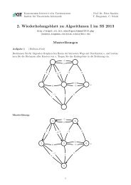
Figure 2 shows a high level view of the merging primitive. In the following we explain
the algorithms for multi sequence selection and parallel merging.
17

Figure 2: Merging four sorted sequences with our algorithm.
5.2 Multiway selection (multi sequence selection)
Given k sorted sequences of length m and of combined length k · m := n, find splitters
split 1 . . . split m such that the sequences are partitioned into the f ·n smallest elements and
the (f − 1) · n largest elements, f ∈ [0, 1]. Varman et al. gave an algorithm with a time
complexity of O(k log(fm)) for this problem [38]. Due to its large constant factors it was
never implemented, at least to our knowledge. In the same paper Varman et al. describe
a simpler variant with a complexity of O(k log(k) log(fm)). This second algorithm is
used by CPU merging routines.
Because we use multi sequence selection to partition sequences into multiple parts,
the selections must be consistent: a selection has to include all elements that any smaller
selection would include. This is no issue if the keys in the input sequences are unique;
selections are then unique as well. But if the greatest key that is included in a selection
is not unique and occurs in more than one input sequence, then several combinations of
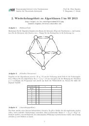
splitters exist which form a valid selection. Figure 3 illustrates selection consistency.
Figure 3: {(1, 0), (2, 0)} – the first selection includes 1 element from the first sequence and
none from the second, the second selection includes 2 elements from the first sequence
and none from the second – is a consistent selection-set. We call it consistent because
every selection in the set includes all smaller selections. This set partitions the sequences
in 2 parts of size 1 and 1 part of size 4. In contrast, {(1, 0), (0, 2)} is inconsistent.
18

Another concern in the presence of duplicate keys is the stability of merging. We
must select duplicate keys in the order in which they appear in the input, otherwise their
relative order may be changed by our partitioning.
We implement two algorithms. The first is due to Vitaly Osipov and akin to the
simpler of the two selection routines devised by Varman et al. The second one lends itself
better to parallelization but has an expected work complexity of O(k log(m) log(m)) –
for uniformly distributed inputs.
Alternative approaches to multi sequence selection include the recursive merging of
splitters used by Thrusts merge sort [34], and random sampling [40]. The latter method
may create partitions of unequal size and therefore may cause load imbalance.
5.2.1 Sequential multi sequence selection
In Algorithm 1 we maintain a lower boundary, upper boundary and a sample element
for each sequence. The sample position and lower boundary are initialized to 0, while
the upper boundary is initialized to m. In addition, a global lower and upper boundary
is stored, indicating how many elements are already selected at least and how many are
selected at most. If the global upper boundary is smaller than the targeted selection size,
then the sequence with the smallest sample element is chosen. If the sample element of
more than one sequence has the smallest value, then the sequence with the lowest index
is chosen. The selection from this sequence is increased, and all boundaries are adjusted
accordingly. Otherwise, the sequence with the greatest sample element is selected and the
selection from it is decreased until the greatest selected element in it is smaller than the
greatest element of which it is known that it belongs to the selection. If the sample element
of more than one sequence has the greatest value, then the sequence with the highest
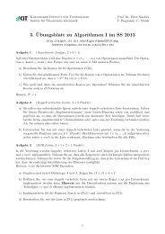
index is chosen. This process is repeated until the global boundaries match. Figure 4
illustrates the process. Breaking ties by sequence index ensures consistent selections that
are also suitable for stable merging. A proof of correctness for Algorithm 1 is provided
in Appendix A.
Figure 4: Algorithm 1 gradually refines its selection in both sequences.
The sample selection is done with a priority queue, which can be implemented e.g.
as a tournament tree. In our GPU implementation we use a parallel reduction instead –
refer to Section 3.4 for a description of the reduction primitive. While a reduction has
a work complexity of O(n) instead of the O(log(n)) achieved by a tournament tree, the
19

latter is completely sequential and therefore a bad match for GPU architectures. Also,
in practice we use parameters for which the reduction is done by a single SIMD group.
As established in Section 3.3 it is then step complexity which matters. For the rest of
the algorithm we have no choice but to execute it sequentially. In Section 5.5 we show
that the sequential execution is affordable when using multi way selection as a sub-step
of merging.
20

Algorithm 1: Sequential multi sequence selection.
/* Global boundaries and sequence boundaries */
U := L := 0 l1 . . . lk := 0 u1 . . . uk := m
/* Samples from all sequences and sample positions. */
s1 := seq1[0] . . . sk := seqk[0] p1 . . . pk := 0
repeat
if U ≤ t then
i := getMinSampleSequenceId(s)
x := si
/* Binary search step, increase selection size. */
n := ui+pi+1
2
if pi = 0 then
L := L + pi − li
U := U + n − pi
else
L := L + 1
U := U + n + 1
si := seqi[n] li := pi
pi := n
else
i := getMaxSampleSequenceId(s)
o := li
low := li+pi high := pi
2
/* Binary search, decrease selection size. */
while low+high
= low and seqi[low] < x do
until U = L
2
li := low
low := low+high
2
end
L := L + li − o
U := U + low − pi
if low = o then
ui := high
si := seq i[low]
pi := low
else
ui := low
21

5.2.2 Parallel multi sequence quick select
Due to its sequential nature Algorithm 1 is not particularly GPU-friendly. Therefore
we investigate an alternative approach, which exposes more parallelism. Its downside is
suboptimal work complexity.
As in Algorithm 1, in Algorithm 2 we maintain a lower and upper boundary for each
sequence. In each step we pick a pivot element uniformly at random from one sequence.
The sequence from which we pick is also selected uniformly at random. We rank the
pivot in each sequence via binary search. If the sum of all ranks is larger than the desired
selection size we use the ranks as new upper boundaries, otherwise we adjust all lower
boundaries. This process is repeated until the correct number of elements is selected.
Algorithm 2: Parallel multi sequence quick select.
/* Let i ∈ 0 . . . p − 1 and p denote the local thread index and thread
count. The number of sequences is is equal to p. The desired
selection size is s. */
li := start of seq i
ui := end of seq i
while p−1
i=0
ri = desired selection sizes do
pick a thread r at random
if i = r then pick a pivot d ∈ [seq i[li], seq i[ui])
ti := binarySearch(d, [seq i[li], seq i[ui]))
if p−1
ti < s then li := ti
i=0
else ui := ti
end
/* Thread i now has the splitter for sequence i in the variable li.
*/
/* The illustration shows how the range from which the pivot is
picked decreases with each step. After 3 steps the desired
selection size is reached in this example. */
Note that this approach only works if each key is unique. If duplicate keys are allowed
it is possible that the correct selection size is never matched. Consider two sequences
where one only contains elements with the key 0, the other one elements with the key 1
of the elements. The pivot will always be either 0 or 1 and each
and our goal is to select 1
4
22

step will select 1 of the elements. To resolve this problem we need two binary searches
2
for each sequence. One search selects the smallest element which is larger than the pivot,
the other selects the largest element which is smaller than the pivot. Then we can stop
iterating as soon as the target size lies between the sum of the lower ranks and the sum
of the upper ranks. A prefix sum over the differences between the upper and lower ranks
(i.e. the number of keys equal to the pivot in each sequence) is used in a last step to adjust
the selection size: starting with the first sequence, the keys in a sequence equal to the
pivot are added to the selection until the desired size is reached. This ensures consistent
selections and enables stable merging. Algorithm 3 depicts the modified procedure. We
investigate several common strategies for picking the pivot element (e.g. median of three).
In our experiments they do not result in significant improvements over picking the pivot
at random.
Algorithm 3: Parallel multi sequence quick select for inputs with duplicate keys.
/* Let i ∈ 0 . . . p − 1 and p denote the local thread index and thread
count. The number of sequences is is equal to p. The desired
selection size is s. */
li := start of seq i
ui := end of seq i
while p−1
end
i=0
ti ≤ s or p−1
i=0
bi ≥ s do
pick a thread r at random
if i = r then pick a pivot d ∈ [seq i[li], seq i[ui])
/* Rank the pivot from above and below. */
ti := binarySearchGreaterThan(d, [seq i[li], seq i[ui]))
bi := binarySearchSmallerThan(d, [seq i[li], seq i[ti]))
if p−1
ti > s then ui := bi
i=0
else if p−1
bi < s then li := bi
i=0
/* Now deal with the keys equal to the last pivot. */
gap := s − p−1
bi
i=0
/* The number of keys equal to the pivot in sequence i. */
xi := ti − bi
scan(x0 . . . xp−1)
if xi+1 ≤ gap then li := ui
else if gap − xi > 0 then li := li + gap − xi
/* Thread i now has the splitter for sequence i in the variable li.
*/
23

5.3 Parallel merging
As described in Section 5.1, routines which allow the threads of a thread block to work
cooperatively on merging two or more sequences are needed. Parallel merging algorithms
which are work-optimal, step-optimal and practical still pose an open problem. Implementations
of Coles optimal parallel merge sort algorithm [11] have so far been unable
to compete with simpler but asymptotically less efficient algorithms. We implement the
well-established odd-even and bitonic merging networks [5], which have a work complexity
of O(n log(n)). In addition we implement hybrid algorithms which combine merging
networks of a fixed size with two-way and four-way merging. These are based on the
ideas of Inoue et al. [21] and can merge sequences with O(n) work. An additional work
factor, logarithmic in the number of threads, is the price for the exposed parallelism.
5.3.1 Comparator networks
Figure 5: A comparator network with two stages. Note that this is not a sorting network.
We provide a brief introduction to comparator networks. A detailed explanation is given
among others by Lang [24]. Comparator networks are sequences of comparator stages.
In turn, comparator stages are sets of disjunct comparator elements. A comparator Ci,j,
where i < j and i, j ∈ [1, n] for a network of size n, compares the input elements ei, ej
and exchanges them if ei > ej. Comparator networks which have the property to sort
their input are termed sorting networks.
Figure 6: A bitonic sorting network of size 8. The input is sorted in 6 steps (from left to
right).
Sorting networks – and analogously also merging networks – have the property that
all comparators in a stage can be executed in parallel. Further, they are data-oblivious
and operate in-place. These properties make them ideal for implementation in SIMD
24

programming models, and also for hardware implementation. The two oldest but still
most practical rules for constructing sorting and merging networks are the odd-even merge
network and the bitonic merge network [5].
5.3.2 Odd-even and bitonic merge
Despite their venerable age of more than 40 years, the bitonic and odd-even merging
network are arguably still the most practical parallel data-oblivious merging algorithms.
They have a step complexity of O(log(n)) and a work complexity of O(n log(n)). Closely
related to these merging networks are sorting networks, which can be constructed among
others by concatenating log(n) merging networks to form a network that sort inputs of
size n in O(log(n) 2 ) steps. For some specific input sizes more efficient sorting networks are
known. It remains an open question whether algorithms for constructing arbitrarily sized
sorting networks which have a better asymptotic work complexity and practical constant
factors do exist. The AKS network [3] achieves optimal step and work complexity – at
the cost of huge constant factors. A comprehensive survey of sorting network research is
given by Knuth [23].
When choosing between different merging networks we have to differentiate between
when we need it to operate on the local memory of a thread block, or where several
thread blocks merge cooperatively via the global memory of the GPU. In the first case,
both bitonic merging and odd-even merging are viable. Odd-even merging can also be
implemented so that it provides a stable merge – the stable variant has larger constant
factors.
Figure 7: A blocked and cyclic mapping between 8 memory addresses and 2 thread blocks,
each consisting of 4 threads.
If global memory access is involved and stable merging is not needed then bitonic
merging becomes more attractive. By alternating between two different data layouts it
is possible to reduce the amount of global memory access by a factor logarithmic in the
size of the local multiprocessor memory, see the work of Ionescu and Schauser [22] for a
proof. Let i denote the index of thread ti in the thread block bj which lies at position
j in the sequence of J thread blocks, each of size I. In the blocked layout, each thread
processes the elements i · j and (i · j) + I. The next log(I) steps are executed in the local
multiprocessor memory. In the cyclic layout the threads of block 1 process the elements
0, J, . . . , I · (J − 1), the threads of block 2 process the elements J + 1, . . . , I · (J − 1) + 1
and so on. See Figure 7 for an illustration. I.e. the cyclic layout involves strided memory
access. Since the local memories are too small to allow for more than 16 steps per layout
25

switch – the number of steps necessary to outweigh the higher cost of strided access – we
always use the blocked layout and perform half of the steps in global memory.
Efficient implementations of merging and sorting networks assume input sizes that are
powers of 2. To deal with arbitrary input sizes the input is either padded with sentinel
elements to the next larger power of 2, or the network is modified so that its last elements
perform a NOOP. Padding incurs some additional index calculations, if multiple bitonic
merges are performed in parallel. For an input of size n it also requires up to n
2 additional
memory. Therefore, the approach that does not need padding is preferable.
A further advantage of bitonic merging lies in the fact that conceptually it does not
merge two sorted sequences into one sorted sequence. It rather transforms a so-called
bitonic sequence into a sorted sequence. A bitonic sequence is a concatenation of an
ascending sequence and a descending sequence, or vice versa. Since only the total length
of the bitonic sequence matters to the network, the overhead for handling the case where
both input sequences are not powers of 2 in length is lower for bitonic merging than it is
for odd-even merging.
Bitonic merging with local memory usage is one of the strategies we take into closer
consideration for our merge primitive. We analyze our implementation in the way that
is outlined in Section 3.3. To merge n elements our implementation uses n log(n)
+ n 2
global memory read operations and the same number of write operations. The number of
compute instructions we count is 14n log(n) + 12n – plus a small constant overhead. On
the Tesla c1060 and the GTX480 device it is therefore generally bounded by computation.
5.3.3 Parallel ranking
Satish et al. [34] use parallel ranking for merging two sequences in parallel: each thread
determines the rank of its element in the other sequence via binary search. Asymptotically,
parallel ranking has the same complexity as the previously described merging
networks. It requires, however, only 2 synchronization barriers instead of log(n) and only
1 write operation per element instead of log(n). Further, parallel ranking also is a stable
merging algorithm. Its main disadvantage is an irregular memory access pattern and
greater memory consumption. Merging networks exchange elements and this requires
just one register as temporary storage for the exchange operation. For parallel ranking
we need two registers for each element a thread processes: one to buffer the element,
the other to memorize its rank. I.e. merging networks require constant register space
per thread, parallel ranking requires register space linear in the number of elements per
thread. Parallel ranking performs notably better on Nvidia Fermi based (e.g. Geforce
GTX480) GPUs than on older Nvidia GPUs; Fermi has more flexible broadcasting for
local memory, which makes parallel binary searches more efficient.
5.3.4 Block-wise merging
To our knowledge Inoue et al. [21] were the first to design a merging algorithm which
exposes parallelism by incorporating a merging network into a sequential merging routine.
Algorithm 4 follows their idea. We merge blocks that have the width b, which is also the
size of a thread block. The resulting work complexity is log(b)n.
For both input sequences one block of size b is buffered; each thread keeps one element
of both sequences in registers. Merging is done in a second buffer of size 2b in the
26

multiprocessors local memory. One step of the merging routine works as follows: thread
0 compares the elements it has stored in registers and writes the result of the comparison
to a variable in the shared local memory. Depending on the result of the comparison,
each thread then pushes its element from one of the sequences into the second buffer.
Effectively, the block from the sequence where the first element is smaller is moved to the
merge buffer. If the first elements are equal to each other, the block from the sequence
which comes first in the input is chosen. The buffer that resides in registers is re-filled
from that sequence. Now the merge buffer contains two sorted sequences of length b – in
each step we re-fill the merge buffers first b positions, the positions b . . . 2b are filled once
at the start in the same manner. E.g. by using a merging network the two sequences
are then merged; the first b positions of the merged result are written to the output.
Obviously, the last b positions of the merge buffer still hold a sorted sequence, which
is merged with a new block in the next step. We repeat this process until both input
sequences are exhausted. A proof of correctness is given in Appendix B.
Stable merging requires a modification: in the beginning the first b positions are filled,
and after each step the elements at the positions b . . . 2b are moved to the first b positions,
and then the positions b . . . 2b are re-filled. This ensures that equal keys do keep their
order. Of course the actual merging routine must be stable as well.
Algorithm 4: Block-wise merging.
/* Let i ∈ 0 . . . p − 1 and p denote the local thread index and thread
count. The merge block size is equal to p. */
for o := i ; o < |input A| + |input B| ; o := o + p do
/* Use a merging network of size 2× block size p. */
merge(buffer 0 . . . buffer 2·p)
output[o] = buffer[i]
/* Thread 0 determines which block to load next. */
if i = 0 then aIsNext := nextA ≤ nextB
/* Put the next element from A or B into the buffer. Advance
position in A or B by p and load the next element. */
if aIsNext then buffer[i] := getNext(input A)
else buffer[i] := getNext(input B)
27

It turns out that the optimum block size should be the SIMD width of the hardware.
Because then the increased work complexity is of no consequence. This disregards two
aspects of the algorithm: first, per block one additional comparison that is made by a
single thread is required. It follows that the amount of sequential work decreases for
larger block sizes. More important, the block size determines how many parallel merging
processes we need to saturate the multiprocessors of the GPU. What we gain here in
efficiency would be outweighed by a more expensive multi sequence selection step.
Refering to Section 3.5 we say that block-wise merging is SIMD-conscious, and that
multi sequence selection is multiprocessor-conscious. A merging routine based on multi
sequence selection and block-wise merging is therefore both SIMD- and multiprocessorconscious.
An important detail of our implementation is that we fill the buffer registers with
sentinels when a sequence is exhausted. A sentinel is a dummy element which is greater
than any element in the input data. The implementation is greatly simplified by using
sentinels. The merging network also need not be able to deal with inputs that are not
powers of 2. This decreases the key range by 1, however, for stable merging; if there are
keys with the same value as the sentinel element the algorithm may write out sentinels.
For non-stable merging we end up using the bitonic merge and for stable merging we
employ parallel ranking, see Section 5.5.4.
Again, we analyze the work complexity of our actual implementation. Per element
our two-way merging implementation takes 12 + 2 · SIMD-width/block-size instructions
outside the merging network, plus a small constant amount of work. Since one global read
and write is required we are left with 6 + SIMD-width/block-size compute instructions
per memory operation, without even considering the work of the merging network. This
implies that our two-way merging is compute-bounded.
5.3.5 Pipelined merging
We explore pipelined merging as a means of decreasing the amount of global memory
access and a possible way to increase work efficiency. Pipelined merging is commonly
used in models with hierarchical memory [16]. Conceptually, one builds a binary tree
of two-way mergers – see Figure 8. Between the levels of the tree buffers are placed
which reside in fast local memory (i.e. local multiprocessor memory for GPUs) and all
mergers except for the ones in the first level are fed from buffers. A tree of 2k − 1
two-way mergers can merge k sequences of combined length n with O(n) accesses to
global memory. Successive two-way merging would incur O(log(k)n) expensive memory
accesses. The limiting factor for implementing a pipelined technique on GPUs is the
available amount of local memory.
28

=>
=>
=>
=>
=>
=>
Figure 8: By using a tree of two-way mergers the merging process is pipelined. Buffers
between the stages of the tree then serve to replace expensive access to global memory
by access to local memory.
To evaluate pipelined merging on GPUs we implement the most basic variant: fourway
merging. Three of our two-way block-wise mergers are combined into a tree, with
buffers between the two levels of the tree. In each step all threads of the thread block
operate one of the mergers on the first level of the tree and then on the head of the
tree. Following the method of analysis we explain in Section 3.3, four-way merge incurs
21 + 4 · SIMD-width/block-size instructions outside the merging networks per element.
In our simplified model it is therefore slightly more efficient than two-way merging. In
comparison to two-way merging, however, our four-way implementation has to place more
variables in local memory instead of registers, requires more registers per thread and also
more buffer space in local memory.
5.3.6 Other parallel merging approaches
Another way of k-way merging uses a priority queue for selecting the next smallest element
from k sequences. The priority queue is commonly implemented as a tournament tree – an
inherently sequential data structure. As an alternative one could use a parallel reduction
instead of a tournament tree. However, the parallel reduction adds an additional work
factor of k. We implement both and find them to deliver abysmal performance in practice,
which is unsurprising. The tournament tree of size k needs to be stored in local memory
to actually reduce the number of accesses to global memory in comparison to two-way
merging. Also, to allow for efficient reading from global memory, an input buffer of 16
elements per sequence must be used. This means only very few tournament tree mergers
can run on a multiprocessor – and only one thread can be used per tournament tree. The
parallel reduction fares just as bad due to its suboptimal work complexity.
Coles merge sort [11] achieves optimal step complexity and work complexity in the
PRAM model. Essentially it uses selection recursively, combined with pipelined merging.
Ding et al. [13] implemented a merging primitive based on Coles idea. The method
proposed by Hagerup and Rüb [18] also merges recursively; Satish et al. [34] derived a
GPU merging algorithm from it.
29
=>

5.4 Sorting by merging
We use our merging routine to construct a sorting algorithm. Sorting by merging has
several advantageous properties. In contrast to distribution-based algorithms, merge sort
incurs strictly sequential memory write access. Merge sort further allows to distribute
work evenly among multiple processors. Lastly, its performance is largely independent of
the input key distribution.
Having a merging primitive available, the only additional complication is producing
the initial set of sorted sequences. We compare four different sorting routines: bitonic
merge sort, quicksort, two-way block-wise merge sort and four-way block-wise merge sort.
All of these can be run with k thread blocks to create k sorted sequences concurrently.
The merge based sorting routines follow the strategies we describe in this section. See
Appendix C for a description of the parallel quicksort algorithm we use.
5.5 Experimental results
To ensure that our results are reproducible we describe our hardware setup and our
methods for generating input data.
5.5.1 Hardware setup
Our test hardware consists of an Intel Q6600 CPU with 8 GiB RAM. We use a Gigabyte
Geforce GTX480. The system runs OpenSUSE 11.1 64 bit Linux. Everything is compiled
with GCC 4.3.4. The Nvidia CUDA 3.0 compiler and runtime environment are used for
all benchmarks. All performance numbers exclude the time for transferring input to the
GPU memory and back to the system main memory. Instead of running time our charts
show the number of elements processed per time, respectively for selecting, merging and
sorting.
5.5.2 Input data
For our analysis we use a commonly accepted set of distributions motivated and described
in [19]. We describe the distributions with the parameters that are used to create 32 bit
keys. 64 bit keys are generated analogously.
Uniform. A uniformly distributed random input in the range [0, 2 32 − 1].
Gaussian. A gaussian distributed random input approximated by setting each value to
an average of 4 random values.
Bucket Sorted. For p ∈ N, the input of size n is split into p blocks, such that the first n
p 2
elements in each of them are random numbers in [0, 232
p
in [ 232 2·232
n
, − 1], and the last p p
p2 elements in [ (p−1)·232
, 2 p
32 ].
−1], the second n
p 2 elements
Staggered. For p ∈ N, the input of size n is split into p blocks such that if the block
index is i ≤ p
2
all its n
p
elements are set to a random number in [(2i−1) 231
p
30
, (2i) 231
p−1 ].

g-Group. For p ∈ N, the input of size n is split into p blocks. Consecutive blocks form
groups consisting of g ∈ N blocks. In group j the first n elements are random
pg
numbers between
(j − 1) g + p
− 1 (mod p) 2
+ 1 231 p and
(j − 1) g + p
(mod p) 2
+ 1 231 n
− 1. The second elements are set to be
p pg
random numbers between
(j − 1) g + p
(mod p) 2
+ 1 231 p and
(j − 1) g + p
+ 1 (mod p) 2
+ 1 231 − 1, and so forth.
p
Deterministic Duplicates. For p ∈ N, the input of size n is split into p blocks, such
that the elements of the first p
p
blocks are set to log n, the elements of the second 2 4
), and so forth.
processors are set to log( n
2
Randomized Duplicates. For p ∈ N, the input of size n is split into p blocks. For each
block an array T is filled with a constant number r of random values set between
n
0 and r − 1 - the sum of these values is S. The first × elements of the input
n
are set to a random value between 0 and r − 1, the next × elements of the
p
input are set to another random value between 0 and r − 1, and so forth.
Sorted. A uniformly distributed random input in the range [0, 2 32 − 1], which has been
sorted.
Our source for uniform random values is the Mersenne Twister [26]. The parameters
for the distributions are set to: p = 240, g = 8 and r = 32. Thus, p corresponds to the
number of scalar processors on an G200-based Tesla c1060 and g to the SIMD width of
its multiprocessors. For r we take the value that was chosen in the original work which
introduced these input distributions. While we perform our final experiments on a Fermibased
Geforce GTX480, which has a different number of scalar processors and a different
SIMD width than G200 has, we stay with the parameters we used in our previous work
to ensure the results are comparable to each other.
In this section we explore the parameter space for the previously explained algorithms.
Then we assemble them into primitives for merging of key-only inputs, stable and nonstable
merging of key-value inputs and for sorting.
Unless stated otherwise we use uniformly distributed 32 bit keys as input. Input
for merging and selection is generated from k · m keys taken from the chosen input
distribution. These k · m keys are split evenly into k sequences which are then sorted.
Note that we only give the results for a meaningful selection of benchmarks. Covering
all or most of the possible combinations of parameters would neither be possible due to
lack of space nor would it be insightful.
5.5.3 Multi sequence selection
At first we take a look at how both multi sequence selection (also called multiway selection)
routines perform for different numbers and lengths of sequences. The number of
splitters is set to 60 – a multiple of the multiprocessor count. The GPU implementation
of Vitaly Osipovs algorithm has a work complexity of O(k 2 log(m)) and a step complexity
of O(k log(k) log(fm)). However, it merely needs O(k log(m)) accesses to global memory.
Our multi sequence quick select implementation has an expected work complexity
31
T [1]
S
p
T [2]
S

of O(k log(m) 2 ), an expected step complexity of O(log(m) 2 ) and it requires expected
O(k log(m) 2 ) accesses to global memory. Since the essential operation of both algorithms
is binary search, there is little computation that could hide memory access latency. We
assume that Osipovs algorithm outperforms the other for large sequences due to its lower
work complexity and bandwidth requirements. The results shown in Figure 9 confirm
our assumption only partly: quick select is faster even for sequences of length 2 20 , if the
input consists of 32 or more sequences.
k * sequence length / time [ns]
32
16
8
4
2
1
0.5
0.25
0.125
2 14
2 15
multi sequence selection rate
pivot k=2
pivot k=8
sequential k=2
sequential k=8
2 16
2 17
2 18
sequence length
2 19
2 20
32
16
8
4
2
1
0.5
0.25
2 14
pivot k=32
pivot k=128
2 15
sequential k=32
sequential k=128
2 16
2 17
2 18
sequence length
Figure 9: Performance (elements processed per time) of sequential and pivot-based multi
sequence selection with varying sequence count k for different input sizes.
We expect our pivot-based selection to perform differently on input distributions that
deviate from the uniform distribution. Osipovs algorithm should be oblivious to the distribution
of the input. Here our assumptions are fully confirmed by our experiments, see
Figure 10. The performance of multi sequence quick select deteriorates to an impractical
level on the staggered distribution. We therefore use Osipovs selection algorithm for our
merging primitive.
32
2 19
2 20

k * sequence length / time [ns]
64
32
16
8
4
2
1
0.5
0.25
0.125
2 14
2 15
pivot bucket
pivot staggered
pivot rand. duplicates
seq bucket
seq staggered
seq rand. duplicates
2 16
2 17
2 18
sequence length
Figure 10: Performance (elements processed per time) of sequential and pivot-based multi
sequence selection for different input distributions, k is set to 32. While the sequential
selection algorithm is oblivous to the input distribution, the pivot-based selection shows
large variance in performance for different input distributions.
The running time for varying numbers of splitters implies a trade off between the
work performed by multi sequence selection and merging. Therefore we will look at it in
the context of the whole merging primitive.
5.5.4 Merging networks
Since the bitonic merge network, the odd-even merge network and parallel ranking all
have the same asymptotic work and step complexity we expect no large variance in
performance between them. We measure their dynamic instruction count for different
thread block sizes, in the context of block-wise two-way merging. The instruction counts
are generated by subtracting the counts from a skeleton program, which performs the
same work but does not execute a merging network, from those of the full program.
At the time of writing the profiling tool for Nvidia GPUs are unable to display instruction
counts for Fermi-based cards. We therefore measure them on a G200-based
card. We expect that the instruction count on Fermi will be lower for parallel ranking,
due to its improved local memory broadcasting capabilities.
Figure 11 shows a comparison between the measured dynamic instruction counts and
our estimates. All estimates are based on counting instructions in our actual implementations,
as described in Section 3.3. For both merging networks our estimates turn out
to be too large. This is no surprise since they assume the worst case, where in each step
all elements have to be exchanged. For parallel ranking the situation is reversed: we do
not account for memory access conflicts that occur during the concurrent binary searches
and thus our instruction counting is too optimistic.
These numbers confirm our hypothesis of block-wise merging being bound by computation.
Even the most favorable case (bitonic merge with 32 threads) takes more than
3 times the number of compute instructions that would be necessary to avoid limitation
by bandwidth on the Tesla c1060.
33
2 19
2 20

algorithm block size 32 64 128 256
odd-even
dynamic instructions 59 65.3 74.3 85.3
estimate: 8 + 15(log(n) − 2) 53 68 83 98
bitonic
dynamic instructions 42.9 50.8 59 70
estimate: 13(log(n) − 1) 52 65 78 91
ranking
dynamic instructions 81.8 93.3 106.4 121.1
estimate: 7 + 11(log(n) − 1) 51 62 73 84
Figure 11: Per-element instruction count estimates and dynamic measurements of oddeven
merge, bitonic merge and parallel ranking for different thread block sizes.
5.5.5 Merging
Here we are interested in the trade off between multi sequence selection and merging for
each of our three merging routines. Our merging algorithms ought to be more efficient at
merging than our multi sequence selection algorithms. Thus we expect the best running
time for two-way and four-way when the work is split among just enough merging thread
blocks to saturate all multiprocessors of the GPU. For bitonic merging this may look
different because of the additional log-factor in its work complexity. We take the average
time per merged element for sequences in the range of [2 12 , 2 20 ]. The number of merging
thread blocks is incremented in steps of 30 – the number of multiprocessors of our GPU.
Our implementations are limited to thread block sizes that are powers of 2; therefore
we measure performance for 32, 64, 128 and 256 threads per block. As multi sequence
selection routine we use Algorithm 1.
The results do match our expectations, see Figure 12. Two-way and four-way merging
perform best when there are exactly as many merging thread blocks as can execute on the
GPU concurrently. We measure peak performance for two-way merging when there are
120 mergers with 128 threads each. The worse performance for merging thread blocks
with 64 and 32 threads is caused by a multiprocessor only executing 8 thread blocks
concurrently. Therefore the GTX480s multiprocessors cannot run enough threads when
using merging thread blocks with less than 128 threads. On the G200-based Tesla c1060
– which requires fewer threads to saturate its multiprocessors – the best performance is
achieved for 64 threads per thread block.
Bitonic merging profits from greater merger counts, since then the sequence parts it
has to merge get smaller. Overall, two-way merging shows the best performance.
34

k * sequence length / time [µs]
k * sequence length / time [µs]
350
300
250
200
150
100
50
0
800
700
600
500
400
300
200
100
0
16 sequences, block size 32
2-way
4-way
bitonic
60 120 180 240
mergers
16 sequences, block size 128
2-way
4-way
bitonic
60 120 180 240
mergers
600
500
400
300
200
100
0
700
600
500
400
300
200
100
16 sequences, block size 64
2-way
4-way
bitonic
60 120 180 240
mergers
16 sequences, block size 256
2-way
4-way
bitonic
60 120 180 240
mergers
Figure 12: Performance of bitonic, two-way and four-way merging for varying numbers
of merging thread blocks. We show the average of the performance for input sequences
with lengths in the range of [2 12 , 2 20 ].
To put the performance of our merging primitive into perspective we compare it to the
merge step of Thrust merge sort [34]. We assume that a merging primitive based on the
merge sort implementation by Ye et al. [40] would perform approximatly as well as ours.
The implementation by Ding et al. [13] is slower than Thrusts merge, according to their
published results. Our primitive uses 120 parallel mergers with 128 threads each. The
non-stable version uses a bitonic merging network, the stable one uses parallel ranking.
Our advantage over the merge from Thrust is on average 35.2% for the non-stable merge
variant and 33.5% for the stable variant. A recent merge sort implementation by Satish
et al. [35], based on selection in two sorted sequences, outperforms a sort based on our
merging primitive by a factor of 2-3. We have, at the time of writing, no access to the
implementation, and therefore do not know how it performs at merging large sequences.
But from its sorting performance we expect it to outperform our merging routine to a
similar degree.
35

merged elements / time [µs]
merging 2 sequences
thrust merge
mss merge
stable mss merge
1400
1200
1000
800
600
400
200
2 17
2 18
2 19
2 20
2 21
2 22
sequence size
Figure 13: Comparison between our stable and non-stable key-value merging primitive
and the merge step from Thrust merge sort.
5.5.6 Sorting
Lastly, we construct a sorting algorithm. We use quicksort, bitonic sort and sorters based
on our two-way and four-way merging algorithms to create a set of sorted sequences from
the input – one thread block creates one sorted sequence. We find that parallel quicksort
outperforms bitonic sort and also sorters based on our two-way and four-way merging
algorithm. We merge these sorted sequences with our merging primitive to obtain the
sorted result.
See Figure 14 for a comparison between our merge sort, GPU Sample Sort and CUD-
PPs radix sort. Merge sort is comfortably beaten by GPU Sample Sort. Note that we
did not spend time to tune merge sort specifically for small inputs. Our implementations
performance for small inputs suffers because we either have to run multi sequence selection
on small sequences (where it is inefficient), or we can run only a small number of
thread blocks to create the initial sorted sequences, leaving multiprocessors unoccupied.
We assume that fundamental algorithmic improvements would be necessary to make
our merge sort strategy competitive. The results of Ye et al. [40] support our argument
– despite a considerably higher amount of architecture-specific optimization their merge
sort implementation, which follows the same overall strategy, achieves similar results.
36
2 23
2 24
2 25

sorted elements / time [µs]
350
300
250
200
150
100
350
300
250
200
150
100
cudpp radix
merge
uniform
50
2 17 2 18 2 19 2 20 2 21 2 22 2 23 2 24 2 25 2 26 2 27
cudpp radix
merge
number of elements
sorted
sample
sample
50
2 17 2 18 2 19 2 20 2 21 2 22 2 23 2 24 2 25 2 26 2 27
350
300
250
200
150
100
cudpp radix
merge
ggroup
sample
50
2 17 2 18 2 19 2 20 2 21 2 22 2 23 2 24 2 25 2 26 2 27
350
300
250
200
150
100
cudpp radix
merge
staggered
sample
50
2 17 2 18 2 19 2 20 2 21 2 22 2 23 2 24 2 25 2 26 2 27
Figure 14: Comparison between quick-multi-selection merge sort, GPU Sample Sort and
CUDPPs radix sort for different key distributions.
6 Revisiting GPU Sample sort
As we are unable to match GPU Sample Sorts performance with our merge sort variants
we attempt to improve GPU Sample Sort, and use it to evaluate the current state of the
OpenCL programming language in Section 7.
6.1 Algorithm overview
Here we describe our original sample sort algorithm.
Randomized sample sort is considered to be one of the most efficient comparisonbased
sorting algorithms for distributed memory architectures. Its sequential version is
best described in pseudocode, see Algorithm 5. The oversampling factor a trades off the
overhead for sorting the splitters and the accuracy of partitioning.
The splitters partition input elements into k buckets delimited by successive splitters,
where k is a power of 2. Each bucket can then be sorted recursively, and their concatenation
forms the sorted output. If M is the size of the input when SmallSort is applied, the
n
algorithm requires logk k-way distribution passes in expectation until the whole input
M
is split into n buckets. Using a small case sorter with a work complexity of O(n log n)
M
leads to an expected work complexity of O(n log n) overall.
37

Algorithm 5: Serial Sample Sort.
SampleSort(e = 〈e1, . . . , en〉, k)
begin
if n < M then return SmallSort(e)
choose a random sample S = S1, S2a . . . , S(k−1)a of e
Sort(S)
〈s0, s1, . . . , sk〉 = 〈−∞, Sa, S2a, . . . , S(k−1)a, ∞〉
for 1 ≤ i ≤ n do
find j ∈ {1, . . . , k}, such that sj−1 ≤ ei ≤ sj
place ei in bucket bj
return Concatenate(SampleSort(b1, k), . . . , SampleSort(bk, k))
end
end
Since the small buckets are sorted in parallel, load-balancing depends on the variance
in size between the buckets, i.e. the quality of the splitter elements. Sufficiently large
random samples yield provably good splitters independent of the input distribution [8].
Due to the high cost of global memory accesses on GPUs, multi-way approaches
are more promising than two-way: each k-way distribution step requires O(n) memory
n
accesses. Expected logk passes are needed until buckets fit into fast GPU local multi-
M
global memory accesses
n
processor memory of size M. Thus, we can expect O(n) logk M
n
instead of the O(n) log2 M
accesses required by two-way sorting. However, the write ac-
cess of a k-way distribution step is not sequential but scattered, reducing the effective
memory bandwidth.
Input
Input
Output
Thread
Blocks
Prefix
Sum
Thread
Blocks
Bucket indices
tl tl tl tl
0
1
k
...
...
...
...
0 1 2 k
Figure 15: An iteration of k-way distribution.
GPU Sample Sort follows a three level strategy. Initially there is one bucket: the whole
input of size n. If a bucket is larger than a threshold M (a size below which further kway
distribution would be inefficient), we apply our k-way distribution procedure to it.
The work of k-way distribution is mostly data-parallel and can be assigned to as many
38
0
1
k

as n thread blocks, where each thread block has up to t threads. When no buckets
t
larger than M are left, the buckets are sorted concurrently with quicksort. Quicksort
switches to odd-even merge sort [5] for buckets that fit into a multiprocessors fast local
memory. In the quicksort step we map one thread block to one bucket. This looks like
a problem, as the amount of work may vary significantly for different thread blocks. In
practice, however, there are typically a lot more thread blocks than multiprocessors and
we achieve sufficient load-balancing.
GPU Sample-Sort’s distribution pass, when the bucket size exceeds a fixed size M,
can be described in 4 steps corresponding to individual kernel launches, see Figure 15.
Step 1. Choose splitters as in Algorithm 5.
Step 2. Each of the p thread blocks computes the bucket indices for all elements in its
tile, counts the number of elements in each bucket and stores this per-block k-entry
histogram in global memory.
Step 3. Perform a prefix sum over the k × p histogram tables stored in a column-major
order to compute global bucket offsets in the output.
Step 4. For its elements each of the p thread blocks computes their local offsets in the
buckets. Finally it stores elements at their proper output positions, using the global
offsets computed in the previous step.
6.2 Algorithm implementation
To reiterate our strategy: buckets larger than some threshold are split via k-way distribution.
Quicksort splits them up further until they fit into the local memory of a thread
block. Then we apply odd-even merge sort. The first two levels of sorting require temporary
space in GPU memory of the size of the input. Additional global memory holds the
prefix sum histogram tables. For keeping track of buckets during the distribution pass
a small amount of CPU memory is required. The size of the prefix sum tables is bound
by a constant and all other temporary storage we use is small enough to be neglected.
Thus, we say our implementation uses space twice the size of the input.
Step 1. We take a random sample S of a · k input elements. A linear congruential
generator is used to synthesize pseudo-random numbers on the GPU. The generator gets
its seed from a Mersenne Twister which runs on the host CPU. We sort S and place each
a-th element of it in the array of splitters bt such that they form a complete binary search
tree with bt[1] = sk/2 as the root. The left child of b[j] is placed at the position 2j and the
right one at 2j + 1, see Algorithm 6. If we find that all keys in S are equal, we memorize
this observation for the other distribution steps. A problem is how to sort S efficiently
on the GPU, as in practice it only contains a few thousand elements. We simply use a
single thread block for sorting S. We run the step in parallel for multiple buckets.
Step 2. Now we split the work among multiple thread blocks: blocks are assigned to
equal-sized parts (tiles) of the bucket. The previously created binary search tree is first
copied into the GPUs cached read-only memory, then loaded into local memory by each
39

thread block. We adopt a tree traversal method that was previously used to prevent
branch mispredictions on commodity CPUs possessing predicated instructions [33], refer
to Algorithm 6. GPUs support predicated instructions as well, see Section 3.2 for details.
Algorithm 6: Serial search tree traversal.
<
s
k/2
s
k/4
< > <
s
3k/4
s
k/8
s
3k/8
s
5k/8
s
7k/8
< > < > < > < >
b
1
b
2
b
3
b
4
b
5
b
6
b
7
b
8
bt = 〈sk/2, sk/4, s3k/4, sk/8, s3k/8, s5k/8, s7k/8 . . .〉
TraverseTree(ei)
begin
j := 1
repeat log k times j := 2j + (ei > bt[j]) // Left or right child?
end
j := j − k + 1 // Bucket index
Each thread loads an element into a register and traverses the binary search tree,
storing its bucket index in local memory. Then, again in local memory, a counter corresponding
to that bucket index is incremented. The counters can be replicated, increasing
parallelism at the expense of local memory space. This procedure is repeated until the
thread blocks whole tile has been processed. The local bucket sizes are written to global
memory, forming a k × p table – p being the number of thread blocks.
Step 3. Performing a prefix sum over bucket size table yields global bucket offsets for
the thread blocks. As efficient prefix sum implementations for GPUs are available we do
not build our own. Instead, we take the one from the Thrust library [34].
Step 4. We recompute the elements bucket indices and scatter them, incrementing
offset counters for each bucket in local memory. An elements output position is given by
its buckets global offset plus that buckets current local counter value. Atomic operations
are used for incrementing the counters.
We still have to consider the previously mentioned degenerate case: all keys in a
sample may be equal. If at the same time their value is greater or equal than that
of any other key in the input, the whole input will be distributed to a single bucket.
As a result we could recurse infinitely on a bucket, failing to ever split it into smaller
buckets. Our solution is to do a partitioning step as in quicksort when we encounter a
degenerated sample. We distinguish between elements that are lesser, equal or greater
40
>
>

than the samples key. Buckets containing elements equal to a samples key need no further
sorting, obviously. Additionally – if a degenerated sample has been detected – two parallel
reductions are performed on the bucket, determining if the bucket contains any keys with
unequal values. Step 4 can be skipped if all keys are equal. This distribution-dependent
behavior works to our advantage. For input distributions with low entropy GPU Sample
Sort can skip superfluous comparisons.
Note that a concise way of avoiding the problem – used for sample sort on other types
of machines [8] – is to tag each key with its position in the input. Thereby one guarantees
that no duplicate keys exist. The high cost of memory operations and the small amount
of local multiprocessor memory make this approach infeasible on GPUs.
This concludes the description of our k-way distribution procedure. The number
of thread blocks can be chosen freely: it allows for a trade-off between the amount of
exposed parallelism on the one hand, and an increased amount of work per thread on the
other hand. The space required for the global offset table and the cost of the prefix sum
also depend on it. Therefore, the k-way distribution procedure is weakly multiprocessorconscious
(see Section 3.5): the number of thread blocks affects the required amount of
work, but this work only makes up a fraction of the total work. It is, however, SIMDoblivious.
Sorting buckets. We delay the sorting of buckets until the whole input is partitioned
into buckets of size at most M. Since the number of buckets grows with the input size,
it is larger than the number of processors most of the time. Therefore, we can use a
single thread block per bucket without sacrificing exploitable parallelism. To improve
load-balancing we schedule buckets for sorting ordered by size. For buckets that are too
large to fit into local memory, we use parallel quicksort to split them up further.
For sequences that fit into local memory, we use the odd-even merge sorting network
[5]. In our experiments we found it to be faster than the bitonic sorting network and
other approaches like a parallel merge sort.
6.3 Exploring bottlenecks
We discuss several bottlenecks of GPU Sample Sort and identify aspects which can be
improved without changing the overall structure of the algorithm. Further, we give performance
numbers for our implementations on the Geforce GTX480. Refer to Section 5.5
for a complete description of our experimental setup.
6.3.1 Sorting networks
The base case sorting with odd-even merge sort makes up approximately 40% of the
overall running time. However, searching for alternatives to the classic (bitonic and oddeven
merge) sorting networks is a deep topic in itself and outside the scope of this work.
Possible candidates include quicksort, merge sort, and also other sorting networks which
have not yet been considered for implementation in the PRAM model.
41

6.3.2 Second level sorting
With M as the bucket size below which the second level sorter is used, the second level
sorters impact on the running time is greatest when M · k m , m ∈ N, is approximately
equal to the input size; then it contributes the most to the sorting process. This shows
in our original implementation: its performance decreases for the input sizes where the
second level quicksort has to sort larger buckets.
We explore two-way merging, four-way merging, and randomized sample sort as alternatives
to quicksort. Merge sort seems attractive because of its sequential memory access
pattern, and because the base case sorting can be performed on tiles that are powers of
two in size – sorting network implementations are more efficient for inputs that have a
size that is a power of 2. In practice we do find that the dynamic instruction count of our
merge sort implementations is at least 40% larger than that of quicksort, and that they
exhibit worse performance. The advantage of sample sort and quicksort is their synergy
with the first level of the sorting process: each k-way distribution step decreases the
entropy within the resulting buckets, and distribution-based sorting gains efficiency for
inputs with low entropy. Further, both sample sort and quicksort are SIMD-oblivious.
We implement a combination of quicksort and sample sort, which is faster and scales
better with the input size than our original implementation, which solely used quicksort.
M is set to 2 18 , the second level sort uses k-way distribution with k = 32, and quicksort
for buckets smaller than 12,000. Since the input size is bounded a small oversampling
factor suffices (we use a = 6); consequently we only have small samples and can sort them
directly with odd-even merge sort. Apart from that the second level sample sort implementation
is based on the algorithm described in Section 6.1. We show the performance
of the different sorting implementations in Figure 16.
6.3.3 k-way distribution
The primary work in a k-way distribution step is done in the kernel that determines the
local bucket sizes and in the kernel that scatters the data to the buckets; the prefix sum
which is performed between these two kernels has a negligible impact on the running
time. Traversal of the binary search tree, atomic increments of the bucket size counters
and scattered writes are the costly parts of k-way distribution.
42

sorted elements / time [µs]
13
12
11
10
9
8
7
6
5
quicksort
sample-quicksort
13
12
11
10
9
8
7
6
5
4
2 11
2 12
quicksort
sample-quicksort
4
2 11
2 12
uniform
2-way merge sort
4-way merge sort
2 13
2 14
2 15
2 16
number of elements
2 13
staggered
2-way merge sort
4-way merge sort
2 14
2 15
2 16
2 17
2 17
2 18
2 18
14
13
12
11
10
9
8
7
6
5
4
2 11
2 12
uniform, 10.78 bits entropy (effective)
quicksort
sample-quicksort
2-way merge sort
4-way merge sort
2 13
quicksort
sample-quicksort
14
13
12
11
10
9
8
7
6
5
4
2 11
2 12
2 13
2 14
sorted
2 14
2 15
2 15
2 16
2-way merge sort
4-way merge sort
Figure 16: A comparison between the performance of thread block quicksort, sample
sort, two-way merge sort and four-way merge sort on the Geforce GTX480. Only a single
thread block is run on the device for this benchmark. Quicksort and sample sort are
more efficient for low entropy inputs. We lower the entropy by combining multiple keys
with a bit-wise and-operation. Combining 4 32 bit keys in this way results in an effective
entropy of 10.78 bits. Each sorter uses odd-even merge sort as base case sorter for input
sizes smaller than 2049.
In our original implementation traversing the binary search tree is already very efficient;
the number of performed comparisons is optimal, no branching occurs and apart
from that a traversal step performs only one read access to local memory, an addition
and a bit-shift operation on data that lies in a register. The only aspect that seems to be
not optimal is the read access to local memory (the binary search tree is stored in local
memory) because there may be access conflicts, which lead to serialized access. Nvidias
Fermi architecture, however, has local memory with broadcasting capabilities. There are
only memory bank conflicts if threads concurrently access different words that belong to
the same memory bank. With 32 memory banks and a word width of 32 bit, the first
6 steps of the search tree traversal are conflict-free. The seventh step exhibits two-way
conflicts, the eighth exhibits four-way conflicts and so on. We use a binary search tree
with 7 levels and therefore only pay one additional instruction in the last step of the
traversal because of conflicts. With a larger tree or with keys longer than 32 bit the
number of conflicts grows, but the overhead is arguably still smaller than it would be
if we would e.g. replicate the binary search tree and use a more complicated indexing
43
2 16
2 17
2 17
2 18
2 18

scheme.
Figure 17: The memory layout of the binary search tree for a GPU with 4 memory
banks and k = 16. Only the last level of the tree contains more than one word in each
memory bank and will therefore exhibit two-way bank conflicts on an architecture with
broadcasting capabilities like Nvidias Fermi.
Since we share bucket size counters between multiple threads, atomic operations are
required to increment them (or explicit serialization). The reason is that there is too
little local memory and register space available to have separate counters for each thread.
For input keys that are distributed in a way that consecutive keys do go into different
buckets, there are no conflicts when incrementing the counters. The worst case occurs
if all keys processed by the same SIMD group go to the same bucket. Replicating the
bucket counters as many times as possible within the limits of the local memory size, so
that fewer threads share counters, improves the worst case behavior.
But using more counters has a price. A higher memory consumption per thread lowers
the number of threads that can run on a multiprocessor, which gives the multiprocessor
a smaller chance to hide memory access latencies. Further, it also decreases the locality
of write access in the scattering kernel as there are more possible write locations. The
locality of write access (and thus the effective bandwidth) is also highest when there are
the most atomic increment conflicts. As a result, depending on the distribution of the
input the kernels shift from being computationally bound to being bandwidth-bound.
We use a different number of threads per bucket counters for step 3 (bucket counting)
and step 4 (scattering) of the k-way distribution routine, refer to Section 6.2. Obviously
the scattering kernel cannot use fewer threads per counter as the bucket counting kernel,
but it can use more threads per counter during scattering. The bucket finding kernel
only executes one sequential read per search tree traversal and atomic increment, making
it more computationally bound than the scattering kernel. In contrast, the scattering
kernel executes an additional scattered write, whose average cost increases with a larger
number of bucket counters. Our implementation uses 8 counters per bucket per thread
block in the bucket finding kernel, and 4 in the scattering kernel. This provides a balance
between a better worst case performance and a lower best case performance.
44

sorted elements / time [µs]
260
240
220
200
180
160
140
120
100
2 17
600
500
400
300
200
100
0
2 17
2 18
2 18
2 19
2 19
uniform
1/1 counters per block
4/4 counters per block
8/4 counters per block
8/2 counters per block
2 20
2 21
2 22
2 23
number of elements
2 20
2 24
detduplicates
1/1 counters per block
4/4 counters per block
8/4 counters per block
8/2 counters per block
2 21
2 22
2 23
2 24
2 25
2 25
2 26
2 26
260
240
220
200
180
160
140
120
100
2 17
280
260
240
220
200
180
160
140
120
100
80
2 17
2 18
2 18
2 19
2 19
2 20
2 20
staggered
1/1 counters per block
4/4 counters per block
8/4 counters per block
8/2 counters per block
2 21
2 22
2 23
2 24
sorted
1/1 counters per block
4/4 counters per block
8/4 counters per block
8/2 counters per block
Figure 18: Performance for different numbers of bucket counters per bucket finding &
scattering thread block, the thread block size is 256. For this benchmark we use the
Geforce GTX480. Replicating the bucket counters results in significantly improved performance
for non-uniformly distributed inputs.
6.4 GPU Sample Sort vs. revised GPU Sample Sort
On average, the revised implementation of GPU Sample Sort is approximately 25% faster
than the original implementation on the Geforce GTX480. More important, it is up to
55% faster for input distributions on which our original implementation performs badly.
See Section 5.5.2 for a description of the key distributions we use in our experiments.
45
2 21
2 22
2 23
2 24
2 25
2 25
2 26
2 26

sorted elements / time [µs]
350
300
250
200
150
cudpp radix
sample (old)
uniform
sample (new)
100
2 17 2 18 2 19 2 20 2 21 2 22 2 23 2 24 2 25 2 26 2 27
600
500
400
300
200
100
cudpp radix
sample (old)
number of elements
detduplicates
sample (new)
0
2 17 2 18 2 19 2 20 2 21 2 22 2 23 2 24 2 25 2 26 2 27
350
300
250
200
150
cudpp radix
sample (old)
bucket
sample (new)
100
2 17 2 18 2 19 2 20 2 21 2 22 2 23 2 24 2 25 2 26 2 27
350
300
250
200
150
100
cudpp radix
sample (old)
sorted
sample (new)
50
2 17 2 18 2 19 2 20 2 21 2 22 2 23 2 24 2 25 2 26 2 27
Figure 19: Original and revised GPU Sample Sorts performance on different 32 bit key
distributions. As a reference we include performance numbers for CUDPPs radix sort
and our merge sort. The better performance on sorted input is largely due to the additional
bucket counter replication in the scattering kernel (step 4 of the k-way distribution
algorithm).
sorted elements / time [µs]
200
180
160
140
120
100
80
60
40
20
2 17
400
350
300
250
200
150
100
50
0
2 17
thrust radix
sample (old)
2 18
uniform
sample (new)
2 19
2 20
2 21
2 22
2 23
number of elements
thrust radix
sample (old)
2 18
2 19
2 20
detduplicates
sample (new)
2 21
2 22
2 23
2 24
2 24
2 25
2 25
220
200
180
160
140
120
100
80
60
40
20
2 17
220
200
180
160
140
120
100
80
60
40
20
2 17
thrust radix
sample (old)
2 18
2 19
2 20
thrust radix
sample (old)
2 18
2 19
2 20
bucket
sample (new)
2 21
2 21
2 22
2 22
2 23
sorted
sample (new)
Figure 20: Original and revised GPU Sample Sorts performance on different 64 bit key
distributions. Thrust radix sort is used as a reference; it is the only competitive GPU
sorting implementation for 64 bit keys available to us.
46
2 23
2 24
2 24
2 25
2 25

sorted elements / time [µs]
260
240
220
200
180
160
140
120
100
80
60
40
2 19
300
250
200
150
100
50
2 19
cudpp radix
thrust merge
2 20
cudpp radix
thrust merge
2 20
uniform
sample (old)
sample (new)
2 21
2 22
number of elements
2 21
2 23
detduplicates
sample (old)
sample (new)
2 22
2 23
2 24
2 24
260
240
220
200
180
160
140
120
100
80
60
40
2 19
260
240
220
200
180
160
140
120
100
80
60
2 19
cudpp radix
thrust merge
2 20
cudpp radix
thrust merge
2 20
2 21
2 21
bucket
sample (old)
sample (new)
2 22
2 22
2 23
sorted
sample (old)
sample (new)
Figure 21: Original and revised GPU Sample Sorts performance on different 32 bit key
distributions with 32 bit values.
6.5 Other possible implementation strategies
Our implementation of sample sort implicitly assumes that the parameter k is chosen as
large as possible within memory limitations, to require as few k-way distribution passes as
possible. As established, scattered writing and sharing bucket counters between threads
are the price we pay for maximizing the parameter k. Limiting k to a smaller value than
we use – for current GPU architectures a choice could be 16 – would allow for different
trade-offs. Counters could be kept in registers for each thread, and it would be feasible to
locally order keys by bucket id prior to scattering them to achieve sequential write access,
or use local memory buffers for each bucket. Such an implementation could be similar
to current GPU radix sort implementations, which usually process 4 bits per pass, and
would be an interesting topic for future work.
7 Converting from Cuda to OpenCL
In this section we shortly compare the OpenCL [2] programming language to Cuda [1],
and describe our experience of implementing GPU Sample Sort in OpenCL. OpenCL is
available for different kinds of multi-core and many-core platforms. We, however, only
look at it in the context of GPU programming.
47
2 23
2 24
2 24

7.1 The OpenCL programming language
OpenCL is very similar to Cuda. GPU kernels are launched by an application that runs
on a CPU host, which also controls memory transfers between its memory and that of the
GPU. In contrast to Cuda, with OpenCL the programmer is responsible for invoking the
compilation of kernels at running time. The compiled kernels can be cached, however, to
avoid unnecessary re-compilation. Therefore an application has to distribute the source
code of its OpenCL kernels in some form, or the developers have to include compiled
kernels for all OpenCL implementations on which they intend to run their application.
An advantage of running time compilation is that it allows for dynamic specialization of
kernel code via preprocessor directives and preprocessor defines, which can be handed to
the compiler.
The syntax for kernels is almost identical, except for key word names. OpenCL forbids
pointer traversal in some places; instead of modifying a pointer one has to use a
base address pointer together with an offset. It is also impossible to declare global memory
pointers that reside in local memory. A more notable difference lies in OpenCLs
synchronization primitives. While Cuda only has one that synchronizes both local and
global memory between threads of a thread block, OpenCL allows to explicitly synchronize
either only local memory, only global memory, or both. Last, Cuda offers C++ style
templates in kernel code. With OpenCL it is possible to emulate template parameters
mostly via preprocessor defines. While this more error-prone and results in code that is
less readable, it is also more powerful because the preprocessor defines can be chosen at
running time in contrast to Cudas template parameters which have to be evaluated at
the applications compile-time. Features like atomic operations, which are not supported
on all GPUs, are exposed in OpenCL via extensions.
Even though OpenCL is based on the same two-level work decomposition as Cuda is
(thread blocks and threads), it allows the programmer to leave out the specification of
the thread block size. One can just specify the total number of threads and leave it to
the OpenCL runtime to determine a suitable thread block size.
7.2 An OpenCL implementation of GPU Sample Sort
As expected, converting Cuda kernels to OpenCL is straightforward. The biggest complication
is our usage of template parameters; but we are able to replace all parameters
which are relevant for performance with preprocessor defines. For longer kernels the
Nvidia OpenCL compiler is, however, less efficient at register allocation than the Cuda
compiler is: an exact conversion of our thread block quicksort requires 22 registers per
thread in OpenCL – the Cuda version only requires 9. Removing one specific code optimization
– a special case for the base case sorting network, where we can omit a loop
in the odd-even merge sort when the number of elements to sort is smaller than or equal
to the number of threads – does lower the register usage in OpenCL to 14 registers per
thread. Further experimentation with the code leads to no additional improvements.
The quicksort kernel suffers from higher register consumption since it is mostly bound by
memory latency, and with a higher register usage per thread fewer threads can run on a
multiprocessor. As a result the access latencies cannot be hidden as much via SMT – see
Section 3.1 for a more detailed explanation.
48

In a few places we are hindered by errors in the current Nvidia OpenCL implementation.
Declaring variables of the type boolean in local memory leads to compilation errors.
Replacing them with integer variables, which should be semantically identical in the C99based
OpenCL, causes our code to malfunction. As a workaround we replace boolean
variables with boolean arrays of size 1. Working with OpenCL is less comfortable than
working with Cuda is, at the time of writing; the Nvidia OpenCL compiler may crash
without giving any meaningful error messages in response to syntactic or semantic errors
in kernel code.
The current Nvidia drivers with support for Fermi-based GPUs (e.g. the Geforce
GTX480) lack stable OpenCL support. We are only able to compare an OpenCL implementation
to a Cuda implementation on a different system, which has an older driver
and a different GPU. This test system has an Intel E8500 CPU with 8 GiB RAM and
a Gainward Geforce 9800GT 1024 MiB. It runs Windows 7 64 bit and the ForceWare
197.45 GPU driver. The Cuda 3.0 compiler is used together with the Visual Studio 2008
C++ compiler. Input data is generated in the same way as described in Section 5.5.2.
Since the Geforce 9800GT lacks atomic operations, we use a different variant of our
GPU Sample Sort implementation. The main difference is that its second level sorter
is quicksort, like in our originally published version, and that it serializes the bucket
counter incrementing in the bucket finding and scattering kernel – refer to Section 6.1
and Section 6.2 for a description of GPU Sample Sorts kernels. The OpenCL and Cuda
implementations use identical parameters, except for quicksort, where we use 128 threads
per block instead of 256 to counter the negative effect of the increased register consumption
of the OpenCL version. Since we use the scan and reduction primitives from the
Thrust [34] library in our Cuda implementation, we also have to implement replacements
for them in OpenCL. To ensure comparability between the OpenCL and Cuda implementation
we also implement our own scan and reduction primitive in Cuda and use these
instead of the ones from Thrust.
On average, the OpenCL implementation reaches 88.7% of the Cuda implementations
performance, see Figure 22. Examining the GPU running times shows a smaller difference
between the OpenCL and Cuda kernels; we conclude that the CPU overhead for
launching kernels is currently larger for OpenCL. Copying data between CPU memory
and GPU memory is also 5% to 15% slower with OpenCL. We expect that – as the
OpenCL compiler and runtime implementation becomes more mature – the difference in
performance between OpenCL and Cuda will decrease further.
49

sorted elements / time [µs]
60
55
50
45
40
35
30
25
20
15
2 17
120
110
100
90
80
70
60
50
40
30
20
10
2 17
uniform
sample (Cuda) sample (OpenCL)
2 18
2 19
2 20
2 21
2 22
2 23
number of elements
detduplicates
sample (Cuda) sample (OpenCL)
2 18
2 19
2 20
2 21
2 22
2 23
2 24
2 24
2 25
2 25
60
55
50
45
40
35
30
25
20
15
2 17
60
55
50
45
40
35
30
25
20
15
2 17
staggered
sample (Cuda) sample (OpenCL)
2 18
2 19
2 20
2 21
2 22
2 23
sorted
sample (Cuda) sample (OpenCL)
Figure 22: Cuda and OpenCL GPU Sample Sorts performance on different 32 bit key
distributions. These benchmarks are performed with a Geforce 9800GT and a modified
version of GPU Sample Sort that does not use atomic operations, consequently the sorting
rates are much lower than in our other experiments. The OpenCL implementation
behaves the same as the Cuda implementation but generally performs worse.
8 Conclusion
Our work on merging resulted in a merging primitive with asymptotically optimal work
complexity and a running time faster than or similar to other GPU merging routines,
except for a hypothetical merging primitive derived from the merge sort algorithm by
Satish et al. [35]. We also demonstrated that sorting and merging are computationally
bound on current generation GPUs. Our multi sequence selection algorithms show that
step complexity should not be over-rated when analyzing GPU algorithms. The selection
algorithm due to Vitaly Osipov also is an example for an algorithm which can be practical
on the GPU even though it contains a substantial amount of sequential work. Further,
our investigation of merging on GPUs made us discover and re-discover several open
problems.
As we noted in Section 5.3.2, the search for practical merging networks with a better
work complexity than the bitonic and the odd-even network has not yielded results for
decades. The discovery of the AKS network [3] with a work complexity of O(n · log(n))
suggests that better networks for merging and sorting may exist. However, the only ad-
50
2 18
2 19
2 20
2 21
2 22
2 23
2 24
2 24
2 25
2 25

vances that have been made are networks which lend themselves to more flexible hardware
implementations – for example the balanced sorting network [14].
Multi-way merging on GPUs also warrants closer investigation. The four-way merging
routine we presented in Section 5.3.5 is certainly not the only feasible implementation
strategy.
In Section 6 we demonstrated incremental improvements to GPU Sample Sort that
lead to 25% higher average performance and elaborated on possible different implementation
strategies for sample sort.
We were successful at porting our implementation to OpenCL, achieving 88.7% of our
Cuda implementations performance. We concluded that OpenCL can be a replacement
for Cuda, although it is not yet as mature and stable as Cuda is. We only tested our
OpenCL implementation on Nvidia hardware; it would be interesting to investigate the
performance of GPU Sample Sort on other platforms that support OpenCL.
Lastly, we argued that there is a lot of work to be done on the topic of abstract machine
models and programming strategies for many-core processors. Finding design strategies
which lead to algorithms that can be adapted and tuned easily for different kinds of
architectures is an important goal. Thus far Merril and Grimshaw [27, 28] described the
most rigorous approach to the tuning of GPU algorithms.
51

A Proof of correctness for sequential multi sequence
selection
A.1 Correctness
To establish the correctness of Algorithm 1, we show that U and L, which always represent
the upper and lower boundary for the size of the current selection c, converge to the target
size t ∈ [0, n], where n is the combined size of all sequences. The precondition for our
proof is that the input sequences are sorted, and that in each step a valid sequence for
increasing or decreasing the current selection is chosen. We show that after each step
after the first step of the algorithm either L ≤ t < U, L < U ≤ t or L = U = t holds
true.
Figure 23: In this case the selection is increased and the previous position in the sequence
is added to the lower boundary.
Let L < U ≤ t; we pick a sequence to increase the selection with, see Figure 23. L
is increased by the difference between the last position in that sequence and the lower
bound of the sequence. U is increased by the difference between the new position and the
last position. Thus, L is now at most as large as U was previously. L can only become
equal to U if U is not increased in the step. Also, for L to become equal to U, U must
be equal to t. If it is not, then we have either not chosen a valid sequence or t is larger
than the total number of elements n. If L is still smaller than U then either L ≤ t < U
or L < U ≤ t hold true, because U ≤ t held true prior to the step.
Figure 24: We decrease the size of the selection. The global upper boundary of the
sequence is decreased.
Let L ≤ t < U; we pick a sequence to decrease the selection with, see Figure 24. L is
increased by the difference between the position of the greatest element in the sequence
that belongs to the final selection. Thus, L ≤ t still holds true and therefore also either
L ≤ t < U, L < U ≤ t or L = U = t.
52

If L = U = t is true the algorithm terminates. The local upper boundaries u1 . . . uk
decrease monotonically. U cannot grow smaller than L or larger than the sum of the local
upper boundaries. The local lower boundaries l1 . . . lk increase monotonically. L cannot
grow larger than t or smaller than the sum of the local lower boundaries. It follows that
U will converge to L, the algorithm will terminate after a finite number of steps, and it
will terminate with a selection of size t.
A.2 Consistency and stability
As established in Section 5.2, selections may be ambiguous in the presence of duplicate
keys. To be exact, multiple selections of a given size exist if the greatest key belonging to
a selection of this size occurs in more than one sequence. We achieve consistent and stable
selections by breaking ties – choosing a sequence when there are multiple sequences whose
sample element has the same key and that key is the smallest or greatest of all sample
element keys – by choosing the sequence with the lowest index for minimum selection,
and choosing the sequence with the greatest index for maximum selection.
Figure 25: A tie between two sequences; key max is the greatest key that is in the selection
and it occurs in two sequences. The bars represent the current selections in these
sequences. All instances of key max in sequence i are selected before any in sequence j are
selected. Vice versa, all instances in sequence j are deselected before any in sequence i are
deselected.
Assume key max is the greatest key that is in the selection and m instances of key max
are in the selection. The sequences are numbered by their order of appearance in the input.
We look at the case where key max occurs x times in sequence i, y times in sequence j,
where i < j, and in no other sequence. It follows from the correctness of the algorithm
that eventually all other sequences are settled and only the boundaries for sequence i and
sequence j remain to be determined. If m ≤ x and any instance of key max in sequence j
is selected, then all instances of key max are selected in sequence i because sequence i takes
precedence over sequence j for minimum selection and thus it takes precedence for increasing
the selection size. It follows that more than m instances of key max are selected and
the selection size is therefore decreased. Here sequence j takes precedence over sequence i;
all instances of key max in sequence j are deselected before any in sequence i are. Thus, if
m ≤ x, all instances of key max that are selected when the algorithm terminates lie in
sequence i. If m > x, then all instances of key max in sequence i are selected and some
in sequence j. Because sequence i precedes sequence j the selection can be used for stable
merging. Also, the selection is a superset of any smaller selection and is therefore consistent.
The same reasoning applies for ties between more than two sequences; they are
53

esolved by successively resolving ties between pairs of sequences in the manner described
here.
B Proof of correctness for block-wise merging
Let X and Y denote the sorted input sequences, xi the element from X at position i
and yj the element from Y at position j. We load blocks of size B into a buffer of size
2 · B. Let xa denote the element behind the most recent block from X, and yb the next
element from Y . After each merge step we output the lower half of the buffer and load
a block from X if xa ≤ yb. Otherwise we load the next block from Y . To show that the
procedure merges X and Y correctly we have to show that the buffer always contains the
next smallest B elements. We prove this by induction.
Figure 26: In the first case both initial blocks are taken from the same sequence, in the
second one is taken from each.
Without loss of generality we differentiate between two base cases which are illustrated
in Figure 26. In the first, the upper half of the buffer is initialized with a block from X
and the next block is also taken from X. Thus, xB ≤ y0 and therefore the buffer contains
the smallest B elements. In the second case the first block is taken from X and the
second one from Y . It follows that the buffer contains B elements from each sequence.
We need at most B elements from X – iff xB−1 ≤ y0 – and vice versa we need at most
B elements from Y . Since the buffer contains exactly B elements from each sequence it
always holds the smallest B elements.
54

Figure 27: The current position in X and Y is denoted by xa and yb. Two blocks of size
B fit into the buffer. The upper half of the buffer contains the elements xa−u . . . xa−1 and
yb−v . . . yb−1, where u + v = B. A new block is taken from X, since xa ≤ yb.
For the inductive step we assume that the merge buffer up to this point always contained
the next B smallest elements. Therefore, for both sequences the distance between
the previous B smallest elements and the current position in that sequence can be at
most B. Otherwise, the previous merge step would have been incorrect. Let u denote
that distance for X and v for Y . Trivially, u + v = B. Without loss of generality, assume
that the next block is taken from X. The next merge will yield an incorrect result only
if more than v elements from Y are among the next B smallest elements. If more than
v elements from Y were needed, then xa > yb. Thus, we would not have taken the next
block from X. This is illustrated in Figure 27. By induction it follows that the buffer
will always contain the next B smallest elements. Thus we have shown the correctness
of block-wise merging.
C CREW PRAM Quicksort
Algorithm 7 is based on the GPU quicksort by Cederman and Tsigas [9]. It operates
on global memory and switches to a different sorting strategy when a partition is small
enough to fit into local multiprocessor memory.
55

Algorithm 7: Parallel Quicksort.
/* Let i ∈ 0 . . . p − 1 and p denote the local thread index and thread
count. */
QSort(e = 〈e1, . . . , en〉)
begin
if n < M then return SmallSort(e)
if i = 0 then pick a pivot d ∈ e
ai := bi := ci := 0
t := e
for i n
p
≤ j ≤ (i + 1) n
p do
if tj < d then ai++
else if tj = d then bi++
else ci++
end
scan(a0 . . . ap−1)
scan(b0 . . . bp−1)
scan(c0 . . . cp−1)
for i n
p
≤ j ≤ (i + 1) n
p do
if tj < d then e[ai] := tj ai++
else if tj = d then e[bi] := tj bi++
else e[ci] := tj ci++
end
return
Concatenate(QSort(〈e1, . . . , eai 〉),〈eai+1, . . . , ebi 〉,QSort(〈ebi+1, . . . , en〉))
end
56

References
[1] CUDA. http://www.nvidia.com/CUDA/.
[2] OpenCL. http://www.khronos.org/opencl/.
[3] M. Ajtai, J. Komlós, and E. Szemerédi. An 0(n log n) sorting network. In STOC ’83:
Proceedings of the fifteenth annual ACM symposium on Theory of computing, pages 1–9,
New York, NY, USA, 1983. ACM.
[4] R. Baraglia, G. Capannini, F. M. Nardini, and F. Silvestri. Sorting using Bitonic network
with CUDA. Universidade Tecnica de Lisboa, 2009.
[5] K. E. Batcher. Sorting networks and their applications. In AFIPS ’68 (Spring): Proceedings
of the April 30–May 2, 1968, spring joint computer conference, pages 307–314, New York,
NY, USA, 1968. ACM.
[6] G. E. Blelloch. Scans as primitive parallel operations. IEEE Trans. Comput., 38(11):1526–
1538, 1989.
[7] G. E. Blelloch. Prefix sums and their applications. Technical Report CMU-CS-90-190,
School of Computer Science, Carnegie Mellon University, Nov. 1990.
[8] G. E. Blelloch, C. E. Leiserson, B. M. Maggs, C. G. Plaxton, S. J. Smith, and M. Zagha.
A comparison of sorting algorithms for the connection machine CM-2. In SPAA ’91:
Proceedings of the third annual ACM symposium on Parallel algorithms and architectures,
pages 3–16, New York, NY, USA, 1991. ACM.
[9] D. Cederman and P. Tsigas. GPU-Quicksort: A practical Quicksort algorithm for graphics
processors. J. Exp. Algorithmics, 14:1.4–1.24, 2009.
[10] J. Chhugani, A. D. Nguyen, V. W. Lee, W. Macy, M. Hagog, Y.-K. Chen, A. Baransi,
S. Kumar, and P. Dubey. Efficient implementation of sorting on multi-core SIMD CPU
architecture. PVLDB, 1(2):1313–1324, 2008.
[11] R. Cole. Parallel merge sort. SIAM J. Comput., 17(4):770–785, 1988.
[12] F. Dehne and H. Zaboli. Deterministic Sample Sort For GPUs. CoRR, abs/1002.4464,
2010.
[13] S. Ding, J. He, H. Yan, and T. Suel. Using graphics processors for high-performance IR
query processing. In WWW ’08: Proceeding of the 17th international conference on World
Wide Web, pages 1213–1214, New York, NY, USA, 2008. ACM.
[14] M. Dowd, Y. Perl, M. Saks, and L. Rudolph. The balanced sorting network. In PODC ’83:
Proceedings of the second annual ACM symposium on Principles of distributed computing,
pages 161–172, New York, NY, USA, 1983. ACM.
[15] R. S. Francis, I. D. Mathieson, and L. Pannan. A fast, simple algorithm to balance a
parallel multiway merge. In PARLE ’93: Proceedings of the 5th International PARLE
Conference on Parallel Architectures and Languages Europe, pages 570–581, London, UK,
1993. Springer-Verlag.
57

[16] M. Frigo, C. E. Leiserson, H. Prokop, and S. Ramachandran. Cache-oblivious algorithms.
In FOCS ’99: Proceedings of the 40th Annual Symposium on Foundations of Computer
Science, Washington, DC, USA, 1999. IEEE Computer Society.
[17] L. Ha, J. Krüger, and C. Silva. Fast Four-Way Parallel Radix Sorting on GPUs. In
Computer Graphics Forum, volume 28, pages 2368–2378. Blackwell Publishing, Dec. 2009.
[18] T. Hagerup and C. Rüb. Optimal merging and sorting on the EREW PRAM. Inf. Process.
Lett., 33(4):181–185, 1989.
[19] D. R. Helman, D. A. Bader, and J. JáJá. A randomized parallel sorting algorithm with an
experimental study. J. Parallel Distrib. Comput., 52(1):1–23, 1998.
[20] B. Huang, J. Gao, and X. Li. An Empirically Optimized Radix Sort for GPU. Parallel and
Distributed Processing with Applications, International Symposium on, 0:234–241, 2009.
[21] H. Inoue, T. Moriyama, H. Komatsu, and T. Nakatani. AA-Sort: A New Parallel Sorting
Algorithm for Multi-Core SIMD Processors. In PACT ’07: Proceedings of the 16th International
Conference on Parallel Architecture and Compilation Techniques, pages 189–198,
Washington, DC, USA, 2007. IEEE Computer Society.
[22] M. F. Ionescu. Optimizing parallel bitonic sort. In IPPS ’97: Proceedings of the 11th
International Symposium on Parallel Processing, pages 303–309, Washington, DC, USA,
1997. IEEE Computer Society.
[23] D. E. Knuth. The art of computer programming, volume 3: (2nd ed.) sorting and searching.
Addison Wesley Longman Publishing Co., Inc., Redwood City, CA, USA, 1998.
[24] H. W. Lang. Sorting networks, 2008.
www.inf.fh-flensburg.de/lang/algorithmen/sortieren/.
[25] N. Leischner, V. Osipov, and P. Sanders. GPU Sample Sort. In Proc. of the 24th International
Symposium on Parallel and Distributed Processing (IPDPS). IEEE Computer
Society, 2010.
[26] M. Matsumoto and T. Nishimura. Mersenne twister: A 623-dimensionally equidistributed
uniform pseudo-random number generator. ACM Transactions on Modeling and Computer
Simulation, 8(1):3–30, 1998.
[27] D. Merril and A. Grimshaw. Parallel scan for stream architectures. Technical report,
University of Virginia, Department of Computer Science, Charlottesville, VA, USA, 2009.
[28] D. Merrill and A. Grimshaw. Revisiting Sorting for GPGPU Stream Architectures. Technical
Report CS2010-03, University of Virginia, Department of Computer Science, Charlottesville,
VA, USA, 2010.
[29] D. R. Musser. Introspective sorting and selection algorithms. Softw. Pract. Exper.,
27(8):983–993, 1997.
[30] L. Natvig. Logarithmic time cost optimal parallel sorting is not yet fast in practice! In
Supercomputing ’90: Proceedings of the 1990 ACM/IEEE conference on Supercomputing,
pages 486–494, Los Alamitos, CA, USA, 1990. IEEE Computer Society Press.
58

[31] H. Peters, O. Schulz-Hildebrandt, and N. Luttenberger. Fast comparison-based in-place
sorting with CUDA. In Eighth International Conference on Parallel Processing and Applied
Mathematics, Sept. 2009.
[32] F. Putze, P. Sanders, and J. Singler. MCSTL: the multi-core standard template library.
In PPoPP ’07: Proceedings of the 12th ACM SIGPLAN symposium on Principles and
practice of parallel programming, pages 144–145, New York, NY, USA, 2007. ACM.
[33] P. Sanders and S. Winkel. Super scalar sample sort. In Proc. of the 12th European Symposium
on Algorithms (ESA), volume 3221 of LNCS, pages 784–796. Springer, 2004.
[34] N. Satish, M. Harris, and M. Garland. Designing efficient sorting algorithms for manycore
GPUs. In IPDPS ’09: Proceedings of the 23th IEEE International Symposium on Parallel&Distributed
Processing, pages 1–10, Washington, DC, USA, 2009. IEEE Computer
Society.
[35] N. Satish, C. Kim, J. Chhugani, A. D. Nguyen, V. W. Lee, D. Kim, and P. Dubey. Fast
sort on CPUs and GPUs: a case for bandwidth oblivious SIMD sort. Technical report,
New York, NY, USA, 2010.
[36] S. Sengupta, M. Harris, Y. Zhang, and J. D. Owens. Scan primitives for GPU computing.
In Proc. ACM SIGGRAPH/EUROGRAPHICS Conference on Graphics Hardware, pages
97–106, 2007.
[37] E. Sintorn and U. Assarsson. Fast parallel GPU-sorting using a hybrid algorithm. J.
Parallel Distrib. Comput., 68(10):1381–1388, 2008.
[38] P. J. Varman, S. D. Scheufler, B. R. Iyer, and G. R. Ricard. Merging multiple lists on
hierarchical-memory multiprocessors. J. Parallel Distrib. Comput., 12(2):171–177, 1991.
[39] H. Wong, M.-M. Papadopoulou, M. Sadooghi-Alvandi, and A. Moshovos. Demystifying
GPU Microarchitecture through Microbenchmarking. In In Proc. IEEE International
Symposium on Performance Analysis of Systems and Software (ISPASS), March 2010,
Washington, DC, USA, 2010. IEEE Computer Society.
[40] X. Ye, D. Fan, W. Lin, N. Yuan, and P. Ienne. High Performance Comparison-Based
Sorting Algorithm on Many-Core GPUs. In Proc. of the 24th International Symposium on
Parallel and Distributed Processing (IPDPS). IEEE Computer Society, 2010.
59