- Page 1 and 2:
Proceedings of the 10 th European C
- Page 3 and 4:
Contents Paper Title Author(s) Page
- Page 5 and 6:
Paper Title Author(s) Page No. A Qu
- Page 7 and 8:
The Project Mobile Game Based Learn
- Page 9 and 10:
Extreme Scaffolding in the Teaching
- Page 11 and 12:
Malaysia); Tuomo Kakkonen (Universi
- Page 13 and 14:
Preface These Proceedings represent
- Page 15 and 16:
Mini Track Chairs Dr Antonios Andre
- Page 17 and 18:
Cornélia Castro is a PhD student i
- Page 19 and 20:
Manuel Frutos-Perez is the Leader o
- Page 21 and 22:
David Mathew works at the Centre fo
- Page 23 and 24:
Research interests include the inve
- Page 25:
Novita Yulianti is a PhD student at
- Page 28 and 29:
Samuel Adu Gyamfi et al. the develo
- Page 30 and 31:
Samuel Adu Gyamfi et al. completion
- Page 32 and 33:
Samuel Adu Gyamfi et al. interactio
- Page 34 and 35:
Survey of Teachers’ use of Comput
- Page 36 and 37:
Babatunde Alabi Alege and Stephen O
- Page 38 and 39:
Babatunde Alabi Alege and Stephen O
- Page 40 and 41:
Babatunde Alabi Alege and Stephen O
- Page 42 and 43:
Issues and Challenges in Implementi
- Page 44 and 45:
Hussein Al-Yaseen et al. 2000/2001
- Page 46 and 47:
Hussein Al-Yaseen et al. phase invo
- Page 48 and 49:
Hussein Al-Yaseen et al. Berthold,
- Page 50 and 51:
Antonios Andreatos Figure 1: Estima
- Page 52 and 53:
Antonios Andreatos exchange applied
- Page 54 and 55:
Antonios Andreatos knowledge space,
- Page 56 and 57:
Figure 5: Video metadata from YouTu
- Page 58 and 59:
Antonios Andreatos The organisatio
- Page 60 and 61:
Constructing a Survey Instrument fo
- Page 62 and 63:
Jonathan Barkand The teacher demon
- Page 64 and 65:
Jonathan Barkand Indicator 2.3: Has
- Page 66 and 67:
References Jonathan Barkand Allen,
- Page 68 and 69:
2. Pedagogical agents Orlando Belo
- Page 70 and 71:
Orlando Belo Type (Tp), the refere
- Page 72 and 73:
3.3 The agent’s architecture Orla
- Page 74 and 75:
Some Reflections on the Evaluation
- Page 76 and 77:
Nabil Ben Abdallah and Françoise P
- Page 78 and 79:
Nabil Ben Abdallah and Françoise P
- Page 80 and 81:
Nabil Ben Abdallah and Françoise P
- Page 82 and 83:
Designing A New Curriculum: Finding
- Page 84 and 85:
Andrea Benn For this new course, it
- Page 86 and 87:
Andrea Benn Technology is already i
- Page 88 and 89:
Andrea Benn To bring about the co-o
- Page 90 and 91:
Latefa Bin Fryan and Lampros Stergi
- Page 92 and 93:
Latefa Bin Fryan and Lampros Stergi
- Page 94 and 95:
Faculty development Online course
- Page 96 and 97:
Latefa Bin Fryan and Lampros Stergi
- Page 98 and 99:
Latefa Bin Fryan and Lampros Stergi
- Page 100 and 101:
Alice Bird being reviewed under the
- Page 102 and 103:
Alice Bird Developing the process m
- Page 104 and 105:
Alice Bird Reflecting on the feasib
- Page 106 and 107:
3.3 Early stage implementation Alic
- Page 108 and 109:
Enhancement of e-Testing Possibilit
- Page 110 and 111:
Martin Cápay et al. of Likert scal
- Page 112 and 113:
Martin Cápay et al. Figure 3 Proce
- Page 114 and 115:
Martin Cápay et al. Figure 4: An e
- Page 116 and 117:
Martin Cápay et al. On the other h
- Page 118 and 119:
Tim Cappelli demand from students t
- Page 120 and 121:
Tim Cappelli at a time and increasi
- Page 122 and 123:
Tim Cappelli forms were processed a
- Page 124 and 125:
Objectives More efficient and faste
- Page 126 and 127:
Digital Educational Resources Repos
- Page 128 and 129:
Cornélia Castro et al. Economic:
- Page 130 and 131:
Cornélia Castro et al. Dimension E
- Page 132 and 133:
Cornélia Castro et al. feedback on
- Page 134 and 135:
Cornélia Castro et al. EdReNe (200
- Page 136 and 137:
Ivana Cechova et al. The influence
- Page 138 and 139:
4. Methodology Ivana Cechova et al.
- Page 140 and 141:
Ivana Cechova et al. Although this
- Page 142 and 143:
8. Conclusion Ivana Cechova et al.
- Page 144 and 145:
Yin Ha Vivian Chan et al. What is s
- Page 146 and 147:
Yin Ha Vivian Chan et al. as a viab
- Page 148 and 149:
Yin Ha Vivian Chan et al. the ILC h
- Page 150 and 151:
The Development and Application of
- Page 152 and 153:
Serdar Çiftci and Mehmet Akif Ocak
- Page 154 and 155:
4.3 Data collection Serdar Çiftci
- Page 156 and 157:
Serdar Çiftci and Mehmet Akif Ocak
- Page 158 and 159:
Table 8: Students’ responses to q
- Page 160 and 161:
An Exploratory Comparative Study of
- Page 162 and 163:
Marija Cubric et al. Web 2.0 tools
- Page 164 and 165:
Marija Cubric et al. Despite all th
- Page 166 and 167:
Marija Cubric et al. Staff profile
- Page 168 and 169:
Marija Cubric et al. In case 3.2, a
- Page 170 and 171:
Marija Cubric et al. Sorcinelli, M.
- Page 172 and 173:
Figure 1: Adaptive eLearning system
- Page 174 and 175:
Blanka Czeczotková et al. knowledg
- Page 176 and 177:
Blanka Czeczotková et al. Figure 2
- Page 178 and 179:
Changing Academics, Changing Curric
- Page 180 and 181:
Christine Davies 2.2.4 Seminars CEL
- Page 182 and 183:
Web Conferencing for us, by us and
- Page 184 and 185:
Mark de Groot, paper (Elluminate 20
- Page 186 and 187:
Mark de Groot, requested. The targe
- Page 188 and 189: Mark de Groot, members of the group
- Page 190 and 191: 6.1 The quick wins Mark de Groot, S
- Page 192 and 193: Tools for Evaluating Students’ Wo
- Page 194 and 195: Jana Dlouhá et al. course was dist
- Page 196 and 197: 2.4 Feedback - student perceptions
- Page 198 and 199: Jana Dlouhá et al. virtual learnin
- Page 200 and 201: 3. Discussion Jana Dlouhá et al. Q
- Page 202 and 203: Jana Dlouhá et al. Sadler, R.D. (2
- Page 204 and 205: Jon Dron et al. Social networking i
- Page 206 and 207: Jon Dron et al. However, it is also
- Page 208 and 209: Jon Dron et al. further in enabling
- Page 210 and 211: 4.3 Differentiated friends Jon Dron
- Page 212 and 213: Experimental Assessment of Virtual
- Page 214 and 215: Michaela Drozdová et al. to the or
- Page 216 and 217: Michaela Drozdová et al. Figure 1:
- Page 218 and 219: Figure 4: Decision tree for visual
- Page 220 and 221: Michaela Drozdová et al. very few
- Page 222 and 223: Glenn Duckworth Other studies have
- Page 224 and 225: Glenn Duckworth merely skim read th
- Page 226 and 227: 8. Finance resources Glenn Duckwort
- Page 228 and 229: Glenn Duckworth was seen as being v
- Page 230 and 231: Francisco Perlas Dumanig et al. Stu
- Page 232 and 233: Francisco Perlas Dumanig et al. in
- Page 234 and 235: Francisco Perlas Dumanig et al. 3.6
- Page 236 and 237: Do you see What I see? - Understand
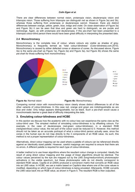
- Page 240 and 241: Colin Egan et al. Figure 5: HCBE's
- Page 242 and 243: Figure 8a: Normal vision LogicWorks
- Page 244 and 245: Researching in the Open: How a Netw
- Page 246 and 247: Antonella Esposito previous edition
- Page 248 and 249: Antonella Esposito However, beyond
- Page 250 and 251: Antonella Esposito Moreno, M. A., F
- Page 252 and 253: Gert Faustmann with an evaluation o
- Page 254 and 255: Gert Faustmann come from the same s
- Page 256 and 257: Gert Faustmann Figure 5: UML class
- Page 258 and 259: Gert Faustmann The learner her/him
- Page 260 and 261: Gert Faustmann (i.e. who has to pro
- Page 262 and 263: Ana Mª Fernández-Pampillón et al
- Page 264 and 265: Ana Mª Fernández-Pampillón et al
- Page 266 and 267: Ana Mª Fernández-Pampillón et al
- Page 268 and 269: Ana Mª Fernández-Pampillón et al
- Page 270 and 271: Ana Mª Fernández-Pampillón et al
- Page 272 and 273: Cognitive Communication 2.0 in the
- Page 274 and 275: Sérgio André Ferreira et al. and
- Page 276 and 277: Sérgio André Ferreira et al. is p
- Page 278 and 279: Sérgio André Ferreira et al. Look
- Page 280 and 281: Sérgio André Ferreira et al. In F
- Page 282 and 283: To What Extent Does a Digital Audio
- Page 284 and 285: Rachel Fitzgerald consideration of
- Page 286 and 287: Rachel Fitzgerald understand, altho
- Page 288 and 289:
Rachel Fitzgerald Although this is
- Page 290 and 291:
Rachel Fitzgerald “The survey was
- Page 292 and 293:
Messages of Support: Using Mobile T
- Page 294 and 295:
Julia Fotheringham and Emily Alder
- Page 296 and 297:
Julia Fotheringham and Emily Alder
- Page 298 and 299:
Table 6: Results for reflective cyc
- Page 300 and 301:
Blended Learning at the Alpen-Adria
- Page 302 and 303:
Gabriele Frankl and Sofie Bitter to
- Page 304 and 305:
Figure 4 Moodle usage among the AAU
- Page 306 and 307:
Gabriele Frankl and Sofie Bitter No
- Page 308 and 309:
Gabriele Frankl and Sofie Bitter wh
- Page 310 and 311:
Evaluating the use of Social Networ
- Page 312 and 313:
Elaine Garcia et al. The process by
- Page 314 and 315:
4.3 Data analysis Elaine Garcia et
- Page 316 and 317:
Elaine Garcia et al. issues of priv
- Page 318 and 319:
8. Conclusions and recommendations
- Page 320 and 321:
Elaine Garcia et al. Nabi, A. (2011
- Page 322 and 323:
Danny Glick and Roni Aviram univers
- Page 324 and 325:
Danny Glick and Roni Aviram most im
- Page 326 and 327:
Danny Glick and Roni Aviram opinion
- Page 328 and 329:
Danny Glick and Roni Aviram Bernard
- Page 330 and 331:
Andrea Gorra and Ollie Jones to hel
- Page 332 and 333:
Andrea Gorra and Ollie Jones Howeve
- Page 334 and 335:
Andrea Gorra and Ollie Jones Figure
- Page 336 and 337:
Andrea Gorra and Ollie Jones Studen
- Page 338 and 339:
Rose Heaney and Megan Anne Arroll A
- Page 340 and 341:
Rose Heaney and Megan Anne Arroll l
- Page 342 and 343:
Rose Heaney and Megan Anne Arroll
- Page 344 and 345:
Rose Heaney and Megan Anne Arroll J
- Page 346 and 347:
Amanda Jefferies learning was furth
- Page 348 and 349:
Amanda Jefferies way in which the o
- Page 350 and 351:
Amanda Jefferies their teaching mat
- Page 352 and 353:
A Methodology for Incorporating Usa
- Page 354 and 355:
Anne Jelfs and Chetz Colwell To try
- Page 356 and 357:
Anne Jelfs and Chetz Colwell We wor
- Page 358 and 359:
The Virtual Learning Environment -
- Page 360 and 361:
John Jessel 2.1 An outline framewor
- Page 362 and 363:
John Jessel teachers who agreed to
- Page 364 and 365:
John Jessel ‘“reduce the clicks
- Page 366 and 367:
Mutlimodal Teaching Through ICT Edu
- Page 368 and 369:
Paraskevi Kanari and Georgios Potam
- Page 370 and 371:
Paraskevi Kanari and Georgios Potam
- Page 372 and 373:
Rosario Kane-Iturrioz Regarding lan
- Page 374 and 375:
Rosario Kane-Iturrioz Figure 2: Exa
- Page 376 and 377:
Rosario Kane-Iturrioz Tests very us
- Page 378 and 379:
Rosario Kane-Iturrioz When compared
- Page 380 and 381:
Rosario Kane-Iturrioz Although the
- Page 382 and 383:
Jana Kapounova et al. eLearning is
- Page 384 and 385:
Jana Kapounova et al. Each dimensio
- Page 386 and 387:
Jana Kapounova et al. project, conn
- Page 388 and 389:
Acknowledgments Jana Kapounova et a
- Page 390 and 391:
Andrea Kelz skills and competences
- Page 392 and 393:
Andrea Kelz web-based activities in
- Page 394 and 395:
Andrea Kelz system. Most other univ
- Page 396 and 397:
Open Courses: The Next big Thing in
- Page 398 and 399:
Kaido Kikkas et al. However, in the
- Page 400 and 401:
Kaido Kikkas et al. generation of w
- Page 402 and 403:
Kaido Kikkas et al. Occasional gue
- Page 404 and 405:
John Knight and Rebecca Rochon guid
- Page 406 and 407:
Evaluation of Quality of Learning S
- Page 408 and 409:
Eugenijus Kurilovas et al. Essalmi
- Page 410 and 411:
Eugenijus Kurilovas et al. (LOs), l
- Page 412 and 413:
Eugenijus Kurilovas et al. Then hie
- Page 414 and 415:
Eugenijus Kurilovas et al. If we lo
- Page 416 and 417:
Models of eLearning: The Developmen
- Page 418 and 419:
Stella Lee et al. Converging (AC a
- Page 420 and 421:
Stella Lee et al. knowledge. Meta k
- Page 422 and 423:
Stella Lee et al. Figure 3: Home pa
- Page 424 and 425:
Stella Lee et al. Azevedo, R., Crom
- Page 426 and 427:
Jake Leith et al. opportunities ble
- Page 428 and 429:
Jake Leith et al. Data was collecte
- Page 430 and 431:
Jake Leith et al. their informal sk
- Page 432 and 433:
Jake Leith et al. For the summative
- Page 434 and 435:
Sophisticated Usability Evaluation
- Page 436 and 437:
Stephanie Linek and Klaus Tochterma
- Page 438 and 439:
Stephanie Linek and Klaus Tochterma
- Page 440 and 441:
Stephanie Linek and Klaus Tochterma
- Page 442 and 443:
Social Networks, eLearning and Inte
- Page 444 and 445:
Birgy Lorenz et al. 135 students p
- Page 446 and 447:
Birgy Lorenz et al. The experts' st
- Page 448 and 449:
Birgy Lorenz et al. Akdeniz, Y. (19
- Page 450 and 451:
Arno Louw programmes, and within th
- Page 452 and 453:
Arno Louw It should be clearly stat
- Page 454 and 455:
Arno Louw somewhat an unwritten con
- Page 456 and 457:
Arno Louw Lecturers assume that le
- Page 458 and 459:
A treasure hunt has to be done to f
- Page 460 and 461:
How to Represent a Frog That can be
- Page 462 and 463:
Robert Lucas Occasionally we will a
- Page 464 and 465:
Robert Lucas Note the need to creat
- Page 466 and 467:
Robert Lucas Figure 5: A model of a
- Page 468 and 469:
Learning by Wandering: Towards a Fr
- Page 470 and 471:
Marie Martin and Michaela Noakes wa
- Page 472 and 473:
Marie Martin and Michaela Noakes Th
- Page 474 and 475:
Marie Martin and Michaela Noakes is
- Page 476 and 477:
Linda Martin et al. across the sect
- Page 478 and 479:
Linda Martin et al. confidence. Alt
- Page 480 and 481:
8. Conclusion Linda Martin et al. T
- Page 482 and 483:
Personalized e-Feedback and ICT Mar
- Page 484 and 485:
Maria-Jesus Martinez-Argüelles et
- Page 486 and 487:
Source: Own elaboration from survey
- Page 488 and 489:
Maria-Jesus Martinez-Argüelles et
- Page 490 and 491:
Maria-Jesus Martinez-Argüelles et
- Page 492 and 493:
1.1 Semantic dimension Maria-Jesús
- Page 494 and 495:
2. Methodology Maria-Jesús Martín
- Page 496 and 497:
Maria-Jesús Martínez-Argüelles e
- Page 498 and 499:
Maria-Jesús Martínez-Argüelles e
- Page 500 and 501:
David Mathew members of staff frigh
- Page 502 and 503:
David Mathew disclose this informat
- Page 504 and 505:
David Mathew baboon smells the wate
- Page 506 and 507:
Peter Mikulecky framing learning, p
- Page 508 and 509:
Peter Mikulecky inhabitants or work
- Page 510 and 511:
Acknowledgements Peter Mikulecky Th
- Page 512 and 513:
Karen Hughes Miller and Linda Leake
- Page 514 and 515:
Karen Hughes Miller and Linda Leake
- Page 516 and 517:
Karen Hughes Miller and Linda Leake
- Page 518 and 519:
An Analysis of Collaborative Learni
- Page 520 and 521:
2.3 Flexible and accessible learnin
- Page 522 and 523:
3.1 Definition of case study Peter
- Page 524 and 525:
Peter Mkhize et al. Basically, soci
- Page 526 and 527:
Peter Mkhize et al. you’ve got yo
- Page 528 and 529:
Ideas for Using Critical Incidents
- Page 530 and 531:
Jonathan Moizer and Jonathan Lean I
- Page 532 and 533:
Jonathan Moizer and Jonathan Lean o
- Page 534:
Jonathan Moizer and Jonathan Lean M