Figure 1. isoclines for
Figure 1. isoclines for
Figure 1. isoclines for

You also want an ePaper? Increase the reach of your titles
YUMPU automatically turns print PDFs into web optimized ePapers that Google loves.
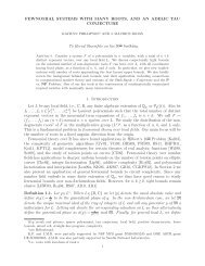
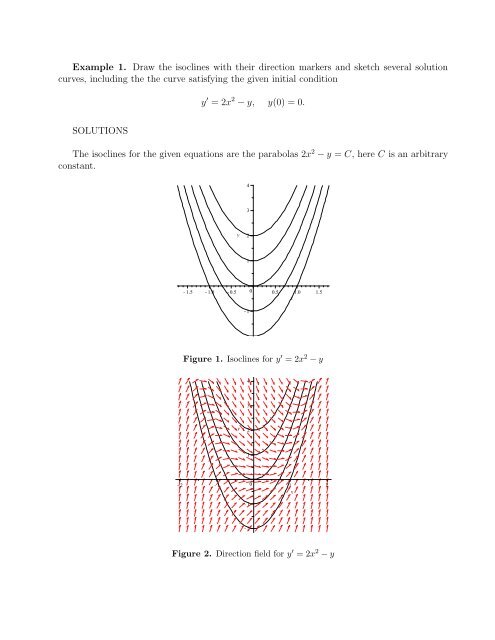
Example <strong>1.</strong> Draw the <strong>isoclines</strong> with their direction markers and sketch several solution<br />
curves, including the the curve satisfying the given initial condition<br />
SOLUTIONS<br />
y ′ = 2x 2 − y, y(0) = 0.<br />
The <strong>isoclines</strong> <strong>for</strong> the given equations are the parabolas 2x 2 − y = C, here C is an arbitrary<br />
constant.<br />
y<br />
4<br />
3<br />
2<br />
1<br />
K<strong>1.</strong>5 K<strong>1.</strong>0 K0.5 0 0.5 <strong>1.</strong>0 <strong>1.</strong>5<br />
x<br />
K1<br />
<strong>Figure</strong> <strong>1.</strong> Isoclines <strong>for</strong> y ′ = 2x 2 − y<br />
y<br />
4<br />
3<br />
2<br />
1<br />
K2 K1 0 1<br />
x<br />
2<br />
K1<br />
K2<br />
<strong>Figure</strong> 2. Direction field <strong>for</strong> y ′ = 2x 2 − y
y(x)<br />
4<br />
3<br />
2<br />
1<br />
K2 K1 0 1<br />
x<br />
2<br />
K1<br />
K2<br />
<strong>Figure</strong> 3. Solutions to y ′ = 2x 2 − y<br />
Section <strong>1.</strong>4 The Approximation Method of Euler<br />
Euler’s method (or the tangent line method) is a procedure <strong>for</strong> constructing approximate<br />
solutions to an initial value problem <strong>for</strong> a first-order differential equation<br />
y ′ = f(x, y),<br />
y(x0) = y0.<br />
The main idea of this method is to construct a polygonal (broken line) approximation to<br />
the solutions of the problem (1).<br />
Assume that the the problem (1) has a unique solution ϕ(x) in some interval centered at x0.<br />
Let h be a fixed positive number (called the step size) and consider the equally spaced points<br />
xn := x0 + nh, n = 0, 1, 2, . . .<br />
The construction of values yn that approximate the solution values ϕ(xn) proceeds as follows.<br />
At the point (x0, y0), the slope of the solution to (1) is given by dy/dx = f(x0, y0). Hence, the<br />
tangent line to the curve y = ϕx at the initial point (x0, y0) is<br />
y − y0 = f(x0, y0)(x − x0), or<br />
y = y0 + f(x0, y0)(x − x0).<br />
Using the tangent line to approximate ϕx, we find that <strong>for</strong> the point x1 = x0 + h<br />
ϕ(x1) ≈ y1 := y0 + f(x0, y0)(x − x0).<br />
Next, starting at the point (x1, y1), we construct the line with slope equal to f(x1, y1). If<br />
we follow the line in stepping from x1 to x2 = x1 + h, we arrive at the approximation<br />
(1)
Repeating the process, we get<br />
ϕ(x2) ≈ y2 := y1 + f(x1, y1)(x − x1).<br />
ϕ(x3) ≈ y3 := y2 + f(x2, y2)(x − x2),<br />
ϕ(x4) ≈ y4 := y3 + f(x3, y3)(x − x3), etc.<br />
This simple procedure is Euler’s method and can be summarized by the recursive <strong>for</strong>mulas<br />
xn+1 := x0 + (n + 1)h, (2)<br />
yn+1 := yn + f(xn, yn)(x − xn), n = 0, 1, 2, . . . (3)<br />
<strong>Figure</strong> <strong>1.</strong> Polygonal-line approximation given by Euler’s method