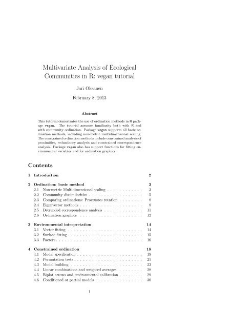
Multivariate Analysis of Ecological Communities in R: vegan tutorial

Multivariate Analysis of Ecological
Communities in R: vegan tutorial
Jari Oksanen
February 8, 2013
Abstract
This tutorial demostrates the use of ordination methods in R package
vegan. The tutorial assumes familiarity both with R and
with community ordination. Package vegan supports all basic ordination
methods, including non-metric multidimensional scaling.
The constrained ordination methods include constrained analysis of
proximities, redundancy analysis and constrained correspondence
analysis. Package vegan also has support functions for fitting environmental
variables and for ordination graphics.
Contents
1 Introduction 2
2 Ordination: basic method 3
2.1 Non-metric Multidimensional scaling . . . . . . . . . . . . 3
2.2 Community dissimilarities . . . . . . . . . . . . . . . . . . 5
2.3 Comparing ordinations: Procrustes rotation . . . . . . . . 8
2.4 Eigenvector methods . . . . . . . . . . . . . . . . . . . . . 8
2.5 Detrended correspondence analysis . . . . . . . . . . . . . 11
2.6 Ordination graphics . . . . . . . . . . . . . . . . . . . . . 12
3 Environmental interpretation 14
3.1 Vector fitting . . . . . . . . . . . . . . . . . . . . . . . . . 14
3.2 Surface fitting . . . . . . . . . . . . . . . . . . . . . . . . . 15
3.3 Factors . . . . . . . . . . . . . . . . . . . . . . . . . . . . . 16
4 Constrained ordination 18
4.1 Model specification . . . . . . . . . . . . . . . . . . . . . . 19
4.2 Permutation tests . . . . . . . . . . . . . . . . . . . . . . . 21
4.3 Model building . . . . . . . . . . . . . . . . . . . . . . . . 23
4.4 Linear combinations and weighted averages . . . . . . . . 28
4.5 Biplot arrows and environmental calibration . . . . . . . . 29
4.6 Conditioned or partial models . . . . . . . . . . . . . . . . 30
1

1 INTRODUCTION
5 Dissimilarities and environment 32
5.1 adonis: Multivariate ANOVA based on dissimilarities . . . 32
5.2 Homogeneity of groups and beta diversity . . . . . . . . . 33
5.3 Mantel test . . . . . . . . . . . . . . . . . . . . . . . . . . 35
5.4 Protest: Procrustes test . . . . . . . . . . . . . . . . . . . 36
6 Classification 36
6.1 Cluster analysis . . . . . . . . . . . . . . . . . . . . . . . . 36
6.2 Display and interpretation of classes . . . . . . . . . . . . 38
6.3 Classified community tables . . . . . . . . . . . . . . . . . 39
1 Introduction
This tutorial demonstrates typical work flows in multivariate ordination
analysis of biological communities. The tutorial first discusses basic unconstrained
analysis and environmental interpretation of their results.
Then it introduces constrained ordination using constrained correspondence
analysis as an example: alternative methods such as constrained
analysis of proximities and redundancy analysis can be used (almost)
similarly. Finally the tutorial describes analysis of species–environment
relations without ordination, and briefly touches classification of communities.
The examples in this tutorial are tested: This is a Sweave document.
The original source file contains only text and R commands: their output
and graphics are generated while running the source through Sweave.
However, you may need a recent version of vegan. This document was
generetated using vegan version 2.0-6 and R version 2.15.1 (2012-06-22).
The manual covers ordination methods in vegan. It does not discuss
many other methods in vegan. For instance, there are several functions
for analysis of biodiversity: diversity indices (diversity, renyi,
fisher.alpha), extrapolated species richness (specpool, estimateR),
species accumulation curves (specaccum), species abundance models (radfit,
fisherfit, prestonfit) etc. Neither is vegan the only R package
for ecological community ordination. Base R has standard statistical
tools, labdsv complements vegan with some advanced methods and provides
alternative versions of some methods, and ade4 provides an alternative
implementation for the whole gamme of ordination methods.
The tutorial explains only the most important methods and shows
typical work flows. I see ordination primarily as a graphical tool, and I
do not show too much exact numerical results. Instead, there are small
vignettes of plotting results in the margins close to the place where you
see a plot command. I suggest that you repeat the analysis, try different
alternatives and inspect the results more thoroughly at your leisure. The
functions are explained only briefly, and it is very useful to check the corresponding
help pages for a more thorough explanation of methods. The
methods also are only briefly explained. It is best to consult a textbook
on ordination methods, or my lectures, for firmer theoretical background.
2

2 ORDINATION: BASIC METHOD
2 Ordination: basic method
2.1 Non-metric Multidimensional scaling
Non-metric multidimensional scaling can be performed using isoMDS function
in the MASS package. This function needs dissimilarities as input.
Function vegdist in vegan contains dissimilarities which are found good
in community ecology. The default is Bray-Curtis dissimilarity, nowadays
often known as Steinhaus dissimilarity, or in Finland as Sørensen index.
The basic steps are:
> library(vegan)
> library(MASS)
> data(varespec)
> vare.dis vare.mds0 stressplot(vare.mds0, vare.dis)
Function stressplot draws a Shepard plot where ordination distances
are plotted against community dissimilarities, and the fit is shown as a
monotone step line. In addition, stressplot shows two correlation like
statistics of goodness of fit. The correlation based on stress is R 2 = 1−S 2 .
The “fit-based R 2 ” is the correlation between the fitted values θ(d) and
ordination distances ˜ d, or between the step line and the points. This
should be linear even when the fit is strongly curved and is often known
as the “linear fit”. These two correlations are both based on the residuals
in the Shepard plot, but they differ in their null models. In linear fit, the
null model is that all ordination distances are equal, and the fit is a flat
horizontal line. This sounds sensible, but you need N − 1 dimensions for
the null model of N points, and this null model is geometrically impossible
in the ordination space. The basic stress uses the null model where all
observations are put in the same point, which is geometrically possible.
Finally a word of warning: you sometimes see that people use correlation
between community dissimilarities and ordination distances. This is dangerous
and misleading since nmds is a nonlinear method: an improved
3
Ordination Distance
0.2 0.4 0.6 0.8 1.0
S = i=j [θ(dij) − ˜ dij] 2
i=j ˜ d2 ij
Non−metric fit, R2 = 0.99
Linear fit, R2 = 0.943
●
●
● ●●●
● ● ●
●
● ●
● ● ● ●
● ●
●
● ●
● ● ●
●
●
●
● ●
●●
●
● ● ● ●
● ●
● ●
● ●
●
● ●●
●
● ● ● ●
●
●
●
● ●
●
● ● ●
● ●●
●
●
●
● ● ● ●
● ●
●
●
●
● ●
●● ●
● ●
●
● ● ●
●
●●
●
● ●
●
●
●
●●
● ●
●
● ●
●
●●
●
●
●
● ●●
● ●
●
●
●
●
●●
●
●
●
●
●
●
●
●
● ● ●
●
●
●
●
●
●
●
●
●
●
●
●
●
●
●
●
●
●
●
●
●
●
●
●
●
●
●
●
●●
●
●
●
●
●
●
● ●
●
●
●
●●
●
●
●
●
● ●
●●
●
●
●
● ●
●
●
●
●
●
●
0.2 0.4 0.6 0.8
Observed Dissimilarity
●

Dim2
NMDS2
−0.4 −0.2 0.0 0.2 0.4
−0.5 0.0 0.5
2.1 Non-metric Multidimensional scaling 2 ORDINATION: BASIC METHOD
28
25
24
22
27
15
14
16
20
23
−0.6 −0.4 −0.2 0.0 0.2 0.4
19
21
Dim1
18
11
7
13
6
Cla.ste
2
Dic.pol
Cet.isl 24
11
Cla.chl
Pin.syl
12
Bar.lyc
Cla.cer
10
9
Poh.nut Pti.cil 21
Cla.bot
Dic.sp
Cet.niv
Emp.nig Vac.vit
1923
4 Cla.ran Cla.unc
Pel.aph
Cla.cri Cla.gra
Pol.pil
Ple.sch
Cet.eri Cal.vul 6 13 Cla.cor Cla.def 20
Cla.fim 15
3 18 Cla.sp 16
Cla.arb Cla.coc
22
7
Pol.jun
14
Bet.pub
28
Vac.myr Led.pal
27
Pol.com Hyl.spl
Ste.sp
5 Dip.mon
Dic.fus
Des.fle
Cla.ama
Ich.eri
Cla.phy
Vac.uli
Nep.arc
25
−0.5 0.0 0.5 1.0
NMDS1
12
10
9
5
4
3
2
ordination with more nonlinear relationship would appear worse with this
criterion.
Functions scores and ordiplot in vegan can be used to handle the
results of nmds:
> ordiplot(vare.mds0, type = "t")
Only site scores were shown, because dissimilarities did not have information
about species.
The iterative search is very difficult in nmds, because of nonlinear relationship
between ordination and original dissimilarities. The iteration
easily gets trapped into local optimum instead of finding the global optimum.
Therefore it is recommended to use several random starts, and
select among similar solutions with smallest stresses. This may be tedious,
but vegan has function metaMDS which does this, and many more
things. The tracing output is long, and we suppress it with trace = 0,
but normally we want to see that something happens, since the analysis
can take a long time:
> vare.mds vare.mds
Call:
metaMDS(comm = varespec, trace = FALSE)
global Multidimensional Scaling using monoMDS
Data: wisconsin(sqrt(varespec))
Distance: bray
Dimensions: 2
Stress: 0.1826
Stress type 1, weak ties
Two convergent solutions found after 20 tries
Scaling: centring, PC rotation, halfchange scaling
Species: expanded scores based on ‘wisconsin(sqrt(varespec))’
> plot(vare.mds, type = "t")
We did not calculate dissimilarities in a separate step, but we gave the
original data matrix as input. The result is more complicated than previously,
and has quite a few components in addition to those in isoMDS results:
nobj, nfix, ndim, ndis, ngrp, diss, iidx, jidx, xinit, istart,
isform, ities, iregn, iscal, maxits, sratmx, strmin, sfgrmn,
dist, dhat, points, stress, grstress, iters, icause, call,
model, distmethod, distcall, data, distance, converged, tries,
engine, species. The function wraps recommended procedures into one
command. So what happened here?
1. The range of data values was so large that the data were square root
transformed, and then submitted to Wisconsin double standardization,
or species divided by their maxima, and stands standardized
to equal totals. These two standardizations often improve the quality
of ordinations, but we forgot to think about them in the initial
analysis.
4

2 ORDINATION: BASIC METHOD 2.2 Community dissimilarities
2. Function used Bray–Curtis dissimilarities.
3. Function run isoMDS with several random starts, and stopped either
after a certain number of tries, or after finding two similar
configurations with minimum stress. In any case, it returned the
best solution.
4. Function rotated the solution so that the largest variance of site
scores will be on the first axis.
5. Function scaled the solution so that one unit corresponds to halving
of community similarity from the replicate similarity.
6. Function found species scores as weighted averages of site scores,
but expanded them so that species and site scores have equal variances.
This expansion can be undone using shrink = TRUE in display
commands.
The help page for metaMDS will give more details, and point to explanation
of functions used in the function.
2.2 Community dissimilarities
Non-metric multidimensional scaling is a good ordination method because
it can use ecologically meaningful ways of measuring community
dissimilarities. A good dissimilarity measure has a good rank order relation
to distance along environmental gradients. Because nmds only uses
rank information and maps ranks non-linearly onto ordination space, it
can handle non-linear species responses of any shape and effectively and
robustly find the underlying gradients.
The most natural dissimilarity measure is Euclidean distance which is
inherently used by eigenvector methods of ordination. It is the distance in
species space. Species space means that each species is an axis orthogonal
to all other species, and sites are points in this multidimensional hyperspace.
However, Euclidean distance is based on squared differences and
strongly dominated by single large differences. Most ecologically meaningful
dissimilarities are of Manhattan type, and use differences instead of
squared differences. Another feature in good dissimilarity indices is that
they are proportional: if two communities share no species, they have a
maximum dissimilarity = 1. Euclidean and Manhattan dissimilarities
will vary according to total abundances even though there are no shared
species.
Package vegan has function vegdist with Bray–Curtis, Jaccard and
Kulczyński indices. All these are of the Manhattan type and use only
first order terms (sums and differences), and all are relativized by site total
and reach their maximum value (1) when there are no shared species
between two compared communities. Function vegdist is a drop-in replacement
for standard R function dist, and either of these functions can
be used in analyses of dissimilarities.
There are many confusing aspects in dissimilarity indices. One is that
same indices can be written with very different looking equations: two
alternative formulations of Manhattan dissimilarities in the margin serve
5
djk = N
djk =
A =
J =
i=1
(xij − xik) 2 Euclidean
N
|xij − xik| Manhattan
i=1
N
i=1
xij
N
min(xij, xik)
i=1
B =
N
i=1
xik
djk = A + B − 2J Manhattan
A + B − 2J
djk =
A + B
A + B − 2J
djk =
A + B − J
djk = 1 − 1
J J
+
2 A B
Bray
Jaccard
Kulczyński

2.2 Community dissimilarities 2 ORDINATION: BASIC METHOD
for A = B dAB = 0
for A = B dAB > 0
dAB = dBA
dAB ≤ dAx + dxB
as an example. Another complication is naming. Function vegdist uses
colloquial names which may not be strictly correct. The default index in
vegan is called Bray (or Bray–Curtis), but it probably should be called
Steinhaus index. On the other hand, its correct name was supposed to be
Czekanowski index some years ago (but now this is regarded as another
index), and it is also known as Sørensen index (but usually misspelt).
Strictly speaking, Jaccard index is binary, and the quantitative variant
in vegan should be called Ruˇzička index. However, vegan finds either
quantitative or binary variant of any index under the same name.
These three basic indices are regarded as good in detecting gradients.
In addition, vegdist function has indices that should satisfy other
criteria. Morisita, Horn–Morisita, Raup–Cric, Binomial and Mountford
indices should be able to compare sampling units of different sizes. Euclidean,
Canberra and Gower indices should have better theoretical properties.
Function metaMDS used Bray-Curtis dissimilarity as default, which
usually is a good choice. Jaccard (Ruˇzička) index has identical rank
order, but has better metric properties, and probably should be preferred.
Function rankindex in vegan can be used to study which of the indices
best separates communities along known gradients using rank correlation
as default. The following example uses all environmental variables in data
set varechem, but standardizes these to unit variance:
> data(varechem)
> rankindex(scale(varechem), varespec, c("euc","man","bray","jac","kul"))
euc man bray jac kul
0.2396 0.2735 0.2838 0.2838 0.2840
are non-linearly related, but they have identical rank orders, and their
rank correlations are identical. In general, the three recommended indices
are fairly equal.
I took a very practical approach on indices emphasizing their ability
to recover underlying environmental gradients. Many textbooks emphasize
metric properties of indices. These are important in some methods,
but not in nmds which only uses rank order information. The metric
properties simply say that
1. if two sites are identical, their distance is zero,
2. if two sites are different, their distance is larger than zero,
3. distances are symmetric, and
4. the shortest distance between two sites is a line, and you cannot
improve by going through other sites.
These all sound very natural conditions, but they are not fulfilled by all
dissimilarities. Actually, only Euclidean distances – and probably Jaccard
index – fulfill all conditions among the dissimilarities discussed here, and
are metrics. Many other dissimilarities fulfill three first conditions and
are semimetrics.
There is a school that says that we should use metric indices, and
most naturally, Euclidean distances. One of their drawbacks was that
6

2 ORDINATION: BASIC METHOD 2.2 Community dissimilarities
they have no fixed limit, but two sites with no shared species can vary
in dissimilarities, and even look more similar than two sites sharing some
species. This can be cured by standardizing data. Since Euclidean distances
are based on squared differences, a natural transformation is to
standardize sites to equal sum of squares, or to their vector norm using
function decostand:
> dis dis d d d

Dimension 2
Procrustes residual
−0.4 −0.2 0.0 0.2 0.4
0.00 0.05 0.10 0.15 0.20 0.25 0.30
2.3 Comparing ordinations: Procrustes rotation 2 ORDINATION: BASIC METHOD
●
●
●
●
●
●
●
●
Procrustes errors
●
●
●
●
●
●
●
●
●
●
−0.4 −0.2 0.0 0.2 0.4 0.6
Dimension 1
Procrustes errors
5 10 15 20
Index
method metric mapping
nmds any nonlinear
mds any linear
pca Euclidean linear
ca Chi-square weighted linear
djk = N
i=1
●
●
(xij − xik) 2
●
●
●
●
2.3 Comparing ordinations: Procrustes rotation
Two ordinations can be very similar, but this may be difficult to see,
because axes have slightly different orientation and scaling. Actually, in
nmds the sign, orientation, scale and location of the axes are not defined,
although metaMDS uses simple method to fix the last three components.
The best way to compare ordinations is to use Procrustes rotation.
Procrustes rotation uses uniform scaling (expansion or contraction) and
rotation to minimize the squared differences between two ordinations.
Package vegan has function procrustes to perform Procrustes analysis.
How much did we gain with using metaMDS instead of default isoMDS?
> tmp dis vare.mds0 pro pro
Call:
procrustes(X = vare.mds, Y = vare.mds0)
Procrustes sum of squares:
0.156
> plot(pro)
In this case the differences were fairly small, and mainly concerned two
points. You can use identify function to identify those points in an
interactive session, or you can ask a plot of residual differences only:
> plot(pro, kind = 2)
The descriptive statistic is “Procrustes sum of squares” or the sum of
squared arrows in the Procrustes plot. Procrustes rotation is nonsymmetric,
and the statistic would change with reversing the order of ordinations
in the call. With argument symmetric = TRUE, both solutions are
first scaled to unit variance, and a more scale-independent and symmetric
statistic is found (often known as Procrustes m 2 ).
2.4 Eigenvector methods
Non-metric multidimensional scaling was a hard task, because any kind
of dissimilarity measure could be used and dissimilarities were nonlinearly
mapped into ordination. If we accept only certain types of dissimilarities
and make a linear mapping, the ordination becomes a simple task of
rotation and projection. In that case we can use eigenvector methods.
Principal components analysis (pca) and correspondence analysis (ca)
are the most important eigenvector methods in community ordination.
In addition, principal coordinates analysis a.k.a. metric scaling (mds) is
used occasionally. Pca is based on Euclidean distances, ca is based on
Chi-square distances, and principal coordinates can use any dissimilarities
(but with Euclidean distances it is equal to pca).
Pca is a standard statistical method, and can be performed with base
R functions prcomp or princomp. Correspondence analysis is not as ubiquitous,
but there are several alternative implementations for that also. In
8

2 ORDINATION: BASIC METHOD 2.4 Eigenvector methods
this tutorial I show how to run these analyses with vegan functions rda
and cca which actually were designed for constrained analysis.
Principal components analysis can be run as:
> vare.pca vare.pca
Call: rda(X = varespec)
Inertia Rank
Total 1826
Unconstrained 1826 23
Inertia is variance
Eigenvalues for unconstrained axes:
PC1 PC2 PC3 PC4 PC5 PC6 PC7 PC8
983.0 464.3 132.3 73.9 48.4 37.0 25.7 19.7
(Showed only 8 of all 23 unconstrained eigenvalues)
> plot(vare.pca)
The output tells that the total inertia is 1826, and the inertia is variance.
The sum of all 23 (rank) eigenvalues would be equal to the total
inertia. In other words, the solution decomposes the total variance into
linear components. We can easily see that the variance equals inertia:
> sum(apply(varespec, 2, var))
[1] 1826
Function apply applies function var or variance to dimension 2 or columns
(species), and then sum takes the sum of these values. Inertia is the sum
of all species variances. The eigenvalues sum up to total inertia. In other
words, they each “explain” a certain proportion of total variance. The
first axis “explains” 983/ 1826 = 53.8 % of total variance.
The standard ordination plot command uses points or labels for
species and sites. Some people prefer to use biplot arrows for species
in pca and possibly also for sites. There is a special biplot function for
this purpose:
PC2
−6 −4 −2 0 2 4 6
Ple.sch 27
28
15 22 25
24
5
7
Cla.arb
13
18
Cla.ran
14
Cal.vul Vac.uli
Ste.sp
11
20
16 Cla.unc Nep.arc Cla.ama Led.pal Dip.mon Pol.com Pol.jun Des.fle Cla.def Bet.pub Pel.aph Poh.nut Cla.coc Cla.gra Cla.phy Cla.cor Cla.bot Cla.cer Dic.pol Cla.fim Bar.lyc Cla.cri Cet.eri Cla.chl Cla.sp Pin.syl Ich.eri Cet.isl Pol.pil Cet.niv Pti.cil
23Dic.fus
Dic.sp Hyl.spl 21 Emp.nig
Vac.myr Vac.vit
6
19
4
−4 −2 0 2 4 6 8 10
> biplot(vare.pca, scaling = -1) −4 −2 0 2 4 6
For this graph we specified scaling = -1. The results are scaled only
when they are accessed, and we can flexibly change the scaling in plot,
biplot and other commands. The negative values mean that species
scores are divided by the species standard deviations so that abundant
and scarce species will be approximately as far away from the origin.
The species ordination looks somewhat unsatisfactory: only reindeer
lichens (Cladina) and Pleurozium schreberi are visible, and all other
species are crowded at the origin. This happens because inertia was variance,
and only abundant species with high variances are worth explaining
(but we could hide this in plot by setting negative scaling). Standardizing
all species to unit variance, or using correlation coefficients instead
of covariances will give a more balanced ordination:
> vare.pca vare.pca
9
PC2
−4 −2 0 2 4
28
Ple.sch
PC1
Cla.gra 18
13 Dip.mon
Cal.vul
Cet.niv4
Cet.eriCla.fim
14
Cla.unc Cla.cer
Cla.def 20
11
16 Cla.cri
23
Cla.cor Pel.aph Bet.pub Bar.lyc
Cla.bot Pti.cil 21
3
2
Pol.jun Nep.arc
15 Dic.fus Dic.pol
Cla.sp
22
19 Pin.syl
12
24 25
Dic.sp
Cet.isl Cla.chl Cla.phy
Led.pal Pol.com
Emp.nig
Cla.ste10
9
27
Des.fle
Vac.myr
Hyl.spl
Cla.arb Cla.ran
Ich.eri 7Ste.sp Vac.uli
Cla.ama Pol.pil Cla.coc
5
6
PC1
3
Vac.vit Poh.nut
12
2
10
9
Cla.ste

PC2
CA2
−2 −1 0 1
−2.0 −1.5 −1.0 −0.5 0.0 0.5 1.0 1.5
2.4 Eigenvector methods 2 ORDINATION: BASIC METHOD
Poh.nut
Cla.coc
Cla.ste Cla.chl
Pin.syl Cet.isl
Cla.sp Cla.gra
Pol.pil Cet.eri Cla.cri Cla.fim
Cla.ran
Cla.arb Ste.sp Dip.mon Cla.unc
Cla.ama Cla.cor
Cal.vul
Cet.niv
Dic.sp
Vac.uli
Dic.fus
Pol.jun
Nep.arc
Vac.vit
Dic.pol
Pti.cil
Bet.pub Bar.lyc
Cla.bot
Emp.nig
Pol.com Led.pal
Pel.aph
11Cla.phy
10
5
23 12
1418
Cla.def
6
13 24
Ich.eri
3
7 15
16 20
4
Cla.cer
2 19
22
Vac.myr
25 Des.fle
Ple.sch Hyl.spl
28
9
27
−1 0 1 2 3
PC1
Led.pal
Vac.myr
9
10
21
Bar.lyc
Bet.pub
28
Hyl.spl
2 12
Cla.phy
Cla.ste
Cet.isl
Cla.chl
19
Pti.cil
Dic.pol
Pol.com
27
Des.fle
Cla.bot
Pin.syl Poh.nut
Ple.sch
Cla.sp
3
Emp.nig
Vac.vit
Dic.sp 24
25
Nep.arc
Pol.jun
Cla.cer
11
Pel.aph
Cla.fim Cla.cor 23
Cla.gra
Cla.cri
15
22
Cla.def
Cla.coc 20 Dic.fus
Cet.eri
Cet.niv
4 Dip.mon Cla.ran
Cla.unc
16
Pol.pil
Cla.ama Cla.arb 18
Vac.uli Cal.vul
5
6
Ste.sp 13
Ich.eri
7
−1 0 1 2
CA1
14
21
Call: rda(X = varespec, scale = TRUE)
Inertia Rank
Total 44
Unconstrained 44 23
Inertia is correlations
Eigenvalues for unconstrained axes:
PC1 PC2 PC3 PC4 PC5 PC6 PC7 PC8
8.90 4.76 4.26 3.73 2.96 2.88 2.73 2.18
(Showed only 8 of all 23 unconstrained eigenvalues)
> plot(vare.pca, scaling = 3)
Now inertia is correlation, and the correlation of a variable with itself is
one. Thus the total inertia is equal to the number of variables (species).
The rank or the total number of eigenvectors is the same as previously.
The maximum possible rank is defined by the dimensions of the data: it
is one less than smaller of number of species or number of sites:
> dim(varespec)
[1] 24 44
If there are species or sites similar to each other, rank will be reduced
even from this.
The percentage explained by the first axis decreased from the previous
pca. This is natural, since previously we needed to “explain” only the
abundant species with high variances, but now we have to explain all
species equally. We should not look blindly at percentages, but the result
we get.
Correspondence analysis is very similar to pca:
> vare.ca vare.ca
Call: cca(X = varespec)
Inertia Rank
Total 2.08
Unconstrained 2.08 23
Inertia is mean squared contingency coefficient
Eigenvalues for unconstrained axes:
CA1 CA2 CA3 CA4 CA5 CA6 CA7 CA8
0.5249 0.3568 0.2344 0.1955 0.1776 0.1216 0.1155 0.0889
(Showed only 8 of all 23 unconstrained eigenvalues)
> plot(vare.ca)
Now the inertia is called mean squared contingency coefficient. Correspondence
analysis is based on Chi-squared distance, and the inertia is
the Chi-squared statistic of a data matrix standardized to unit total:
> chisq.test(varespec/sum(varespec))
Pearsons Chi-squared test
data: varespec/sum(varespec)
X-squared = 2.083, df = 989, p-value = 1
10

2 ORDINATION: BASIC METHOD 2.5 Detrended correspondence analysis
You should not pay any attention to P -values which are certainly misleading,
but notice that the reported X-squared is equal to the inertia
above.
Correspondence analysis is a weighted averaging method. In the graph
above species scores were weighted averages of site scores. With different
scaling of results, we could display the site scores as weighted averages of
species scores:
> plot(vare.ca, scaling = 1)
We already saw an example of scaling = 3 or symmetric scaling in pca.
The other two integers mean that either species are weighted averages of
sites (2) or sites are weighted averages of species (1). When we take
weighted averages, the range of averages shrinks from the original values.
The shrinkage factor is equal to the eigenvalue of ca, which has a
theoretical maximum of 1.
2.5 Detrended correspondence analysis
Correspondence analysis is a much better and more robust method for
community ordination than principal components analysis. However,
with long ecological gradients it suffers from some drawbacks or “faults”
which were corrected in detrended correspondence analysis (dca):
Single long gradients appear as curves or arcs in ordination (arc
effect): the solution is to detrend the later axes by making their
means equal along segments of previous axes.
Sites are packed more closely at gradient extremes than at the centre:
the solution is to rescale the axes to equal variances of species
scores.
Rare species seem to have an unduly high influence on the results:
the solution iss to downweight rare species.
All these three separate tricks are incorporated in function decorana
which is a faithful port of Mark Hill’s original programme with the same
name. The usage is simple:
> vare.dca vare.dca
Call:
decorana(veg = varespec)
Detrended correspondence analysis with 26 segments.
Rescaling of axes with 4 iterations.
DCA1 DCA2 DCA3 DCA4
Eigenvalues 0.524 0.325 0.2001 0.1918
Decorana values 0.525 0.157 0.0967 0.0608
Axis lengths 2.816 2.205 1.5465 1.6486
> plot(vare.dca, display="sites")
11
CA2
−2 −1 0 1 2
Cet.isl
Cla.phy Cla.chl
Cla.ste
9
21
28
10
Pin.syl Poh.nut
Ple.sch
2Cla.sp
12
27
Emp.nig 19
Vac.vit
Dic.sp
Nep.arc
3
Pol.jun 24 25
Cla.cer 11 Pel.aph 23
Cla.fim Cla.cor 15 22
20
4
Cla.gra 16
Cla.cri Cla.def
Cla.coc 18
Dic.fus
Cet.eri 14
Cet.niv
6 13
Dip.mon
Cla.unc
Cla.ran 7
Pol.pil 5
Cla.ama Cla.arb
Vac.uli Cal.vul
Ste.sp
Ich.eri
Bar.lyc
Bet.pub
Led.pal
Vac.myr
Hyl.spl
Pti.cil
Dic.pol
Pol.com
Des.fle
Cla.bot
−2 −1 0 1 2 3
CA1

DCA2
−1.0 −0.5 0.0 0.5 1.0
2.6 Ordination graphics 2 ORDINATION: BASIC METHOD
10
9
2
3
4
12
5
11
18
6
13
7
19
−1.0 −0.5 0.0 0.5 1.0 1.5
21
DCA1
23
20
14
16
15
27
22
24
25
28
Function decorana finds only four axes. Eigenvalues are defined as
shrinkage values in weighted averages, similarly as in cca above. The
“Decorana values” are the numbers that the original programme returns
as “eigenvalues” — I have no idea of their possible meaning, and they
should not be used. Most often people comment on axis lengths, which
sometimes are called “gradient lengths”. The etymology is obscure: these
are not gradients, but ordination axes. It is often said that if the axis
length is shorter than two units, the data are linear, and pca should be
used. This is only folklore and not based on research which shows that
ca is at least as good as pca with short gradients, and usually better.
The current data set is homogeneous, and the effects of dca are not
very large. In heterogeneous data with a clear arc effect the changes often
are more dramatic. Rescaling may have larger influence than detrending
in many cases.
The default analysis is without downweighting of rare species: see help
pages for the needed arguments. Actually, downweight is an independent
function that can be used with cca as well.
There is a school of thought that regards dca as the method of choice
in unconstrained ordination. However, it seems to be a fragile and vague
back of tricks that is better avoided.
2.6 Ordination graphics
We have already seen many ordination diagrams in this tutorial with one
feature in common: they are cluttered and labels are difficult to read.
Ordination diagrams are difficult to draw cleanly because we must put a
large number of labels in a small plot, and often it is impossible to draw
clean plots with all items labelled. In this chapter we look at producing
cleaner plots. For this we must look at the anatomy of plotting functions
in vegan and see how to gain a better control of default functions.
Ordination functions in vegan have their dedicated plot functions
which provides a simple plot. For instance, the result of decorana is
displayed by function plot.decorana which behind the scenes is called
by our plot function. Alternatively, we can use function ordiplot which
also works with many non-vegan ordination functions, but uses points
instead of text as default. The plot.decorana function (or ordiplot)
actually works in three stages:
1. It draws an empty plot with labelled axes, but with no symbols for
sites or species.
2. It uses functions text or points to add species to the empty frame.
If the user does not ask specifically, the function will use text in
small data sets and points in large data sets.
3. It adds the sites similarly.
For better control of the plots we must repeat these stages by hand: draw
an empty plot and then add sites and/or species as desired.
In this chapter we study a difficult case: plotting the Barro Colorado
Island ordinations.
12

2 ORDINATION: BASIC METHOD 2.6 Ordination graphics
> data(BCI)
This is a difficult data set for plotting: it has 225 species and there is no
way of labelling them all cleanly – unless we use very large plotting area
with small text. We must show only a selection of the species or small
parts of the plot. First an ordination with decorana and its default plot:
> mod plot(mod)
There is an additional problem in plotting species ordination with these
data:
> names(BCI)[1:5]
[1] "Abarema.macradenium" "Acacia.melanoceras"
[3] "Acalypha.diversifolia" "Acalypha.macrostachya"
[5] "Adelia.triloba"
The data set uses full species names, and there is no way of fitting those
in ordination graphs. There is a utility function make.cepnames in vegan
to abbreviate Latin names:
> shnam shnam[1:5]
[1] "Abarmacr" "Acacmela" "Acaldive" "Acalmacr" "Adeltril"
The easiest way to selectively label species is to use interactive identify
function: when you click next to a point, its label will appear on the
side you clicked. You can finish labelling clicking the right mouse button,
or with handicapped one-button mouse, you can hit the esc key.
> pl identify(pl, "sp", labels=shnam)
There is an “ordination text or points” function orditorp in vegan.
This function will label an item only if this can be done without overwriting
previous labels. If an item cannot be labelled with text, it will be
marked as a point. Items are processed either from the margin toward
the centre, or in decreasing order of priority. The following gives higher
priority to the most abundant species:
> stems plot(mod, dis="sp", type="n")
> sel

DCA2
−4 −2 0 2 4
Casecomm
Alchlati
Abarmacr
Ochrpyra Schipara Pachquin
Pourbico Ficucolu Sipaguia Laetproc Lafopuni Cupacine Micoelat
Myrcgatu Garcmadr Micohond Entescho
Tricgale Desmpana MicoaffiPachsess
Ficuyopo
Hampappe Guargran
Ormoamaz Cuparufe
Cedrodor Ingaspec Spacmemb Solahaye Coluglan Chimparv
Margnobi
Alibedul Talinerv
Heisacum Nectpurp Chamschi Tricgiga Chlotinc
Ingaoers
Ficupope
Pipereti Acalmacr
Poutfoss Tocopitt
Taliprin Ingapunc Ficuinsi
Ingaruiz Ormomacr
Tetrjoha
Coccmanz Pseusept
Theocaca Zuelguid Nectline Eugegala Vochferr
Acaldive
Ficucost Acacmela
Ingalaur
Ormococc
Myrofrut Banaguia Psycgran
Ficumaxi Ficuobtu
Psidfrie
Caseguia
Vismbacc Cupalati
Sapibroa Marilaxi Ficutrig
Licaplat Cespmacr
Chryecli Thevahou
Ingaumbe
Perexant
Sipapauc Ingacocl
Nectciss Ocotpube Laettham
Zantjuni Zantpana
Cocccoro
Cupasylv Plateleg
Phoecinn Licahypo
Diptpana
Mosagarw Cecrobtu Protpana
Platpinn
Turpocci Sponradl Sponmomb
Aegipana Laciaggr
Ocotcern Astrgrav
Sympglob Eugenesi Erytmacr Tabeguay Micoarge
Annospra Cordalli
Termamaz
Poutstip Tremmicr Ceibpent
Lacmpana Couscurv Elaeolei
Ingagold Ingasapi
Ficutond Maytschi Trataspe Calolong
Celtschi Troprace Chrycain
Sapiglan
Apeitibo
Erytcost Andiiner
Guarfuzz
Diosarta Sterapet Allopsil Casesylv
Lindlaur
Guazulmi
Soroaffi Geniamer
Attabuty
Hyeralch
Sloatern
Inganobi
Ocotoblo Caseacul
Taberose Aspicrue
Viromult AnacexceCavaplat
Macrrose
Tropcauc
Ingaacum
Termoblo
Picrlati
Posolati Ingapezi
Pterrohr
Socrexor
Cordbico Dendarbo
Cecrinsi
Simaamar
Zantekma Jacacopa Tabearbo Priocopa Casearbo
Unonpitt
Chryarge Casselli Lonclati
Maqucost Protcost Hassflor
Apeiaspe
Guatdume Oenomapo
Virosebi Swarochn Tricpall
Tachvers Crotbill Poutreti Swargran Eugeoers Faraocci Trictube
Beilpend
Guetfoli Alseblac
Guapstan Randarma
Tetrpana
Ingamarg Brosalic Eugecolo Alchcost Adeltril
Heisconc Garcinte Luehseem Gustsupe
Poularma Quaraste
Astrstan
Ocotwhit Virosuri CordlasiTripcumi
Hirttria Prottenu Guarguid
Xylomacr Huracrep
Drypstan
Brosguia
Hirtamer
Quasamar
Amaicory
Senndari Zantsetu
−6 −4 −2 0 2 4 6
DCA1
3 ENVIRONMENTAL INTERPRETATION
> plot(mod, dis="sp", type="n")
> ordilabel(mod, dis="sp", lab=shnam, priority = stems)
Finally, there is function ordipointlabel which uses both points and
labels to these points. The points are in fixed positions, but the labels are
iteratively located to minimize their overlap. The Barro Colorado Island
data set has much too many names for the ordipointlabel function, but
it can be useful in many cases.
In addition to these automatic functions, function orditkplot allows
editing of plots. It has points in fixed positions with labels that can
be dragged to better places with a mouse. The function uses different
graphical toolset (Tcl/Tk) than ordinary R graphics, but the results can
be passed to standard R plot functions for editing or directly saved as
graphics files. Moreover, the ordipointlabel ouput can be edited using
orditkplot.
Functions identify, orditorp, ordilabel and ordipointlabel may
provide a quick and easy way to inspect ordination results. Often we need
a better control of graphics, and judicuously select the labelled species.
In that case we can first draw an empty plot (with type = "n"), and
then use select argument in ordination text and points functions. The
select argument can be a numeric vector that lists the indices of selected
items. Such indices are displayed from identify functions which can be
used to help in selecting the items. Alternatively, select can be a logical
vector which is TRUE to selected items. Such a list was produced invisibly
from orditorp. You cannot see invisible results directly from the method,
but you can catch the result like we did above in the first orditorp call,
and use this vector as a basis for fully controlled graphics. In this case
the first items were:
> sel[1:14]
Abarmacr Acacmela Acaldive Acalmacr Adeltril Aegipana Alchcost
FALSE FALSE FALSE FALSE FALSE FALSE FALSE
Alchlati Alibedul Allopsil Alseblac Amaicory Anacexce Andiiner
TRUE FALSE FALSE FALSE TRUE TRUE FALSE
3 Environmental interpretation
It is often possible to “explain” ordination using ecological knowledge on
studied sites, or knowledge on the ecological characteristics of species.
Usually it is preferable to use external environmental variables to interpret
the ordination. There are many ways of overlaying environmental
information onto ordination diagrams. One of the simplest is to change
the size of plotting characters according to an environmental variables
(argument cex in plot functions). The vegan package has some useful
functions for fitting environmental variables.
3.1 Vector fitting
The most commonly used method of interpretation is to fit environmental
vectors onto ordination. The fitted vectors are arrows with the interpretation:
14

3 ENVIRONMENTAL INTERPRETATION 3.2 Surface fitting
The arrow points to the direction of most rapid change in the the
environmental variable. Often this is called the direction of the
gradient.
The length of the arrow is proportional to the correlation between
ordination and environmental variable. Often this is called the
strength of the gradient.
Fitting environmental vectors is easy using function envfit. The
example uses the previous nmds result and environmental variables in
the data set varechem:
> data(varechem)
> ef ef
***VECTORS
NMDS1 NMDS2 r2 Pr(>r)
N -0.0573 -0.9984 0.25 0.036 *
P 0.6197 0.7848 0.19 0.101
K 0.7665 0.6423 0.18 0.114
Ca 0.6852 0.7283 0.41 0.003 **
Mg 0.6325 0.7745 0.43 0.004 **
S 0.1914 0.9815 0.18 0.132
Al -0.8716 0.4902 0.53 0.001 ***
Fe -0.9360 0.3520 0.45 0.001 ***
Mn 0.7987 -0.6017 0.52 0.001 ***
Zn 0.6176 0.7865 0.19 0.108
Mo -0.9031 0.4294 0.06 0.512
Baresoil 0.9249 -0.3803 0.25 0.055 .
Humdepth 0.9328 -0.3604 0.52 0.003 **
pH -0.6480 0.7617 0.23 0.060 .
---
Signif. codes: 0 ‘***’ 0.001 ‘**’ 0.01 ‘*’ 0.05 ‘.’ 0.1 ‘ ’ 1
P values based on 999 permutations.
The first two columns give direction cosines of the vectors, and r2 gives
the squared correlation coefficient. For plotting, the axes should be scaled
by the square root of r2. The plot function does this automatically, and
you can extract the scaled values with scores(ef, "vectors"). The
significances (Pr>r), or P -values are based on random permutations of
the data: if you often get as good or better R 2 with randomly permuted
data, your values are insignificant.
You can add the fitted vectors to an ordination using plot command.
You can limit plotting to most significant variables with argument p.max.
As usual, more options can be found in the help pages.
> plot(vare.mds, display = "sites")
> plot(ef, p.max = 0.1)
3.2 Surface fitting
Vector fitting is popular, and it provides a compact way of simultaneously
displaying a large number of environmental variables. However, it implies
15
NMDS2
−0.4 −0.2 0.0 0.2 0.4
●
●
Al
Fe
●
●
●
pH
●
●
●
●
●
●
●
N
●
●
●
● ●
●
−0.4 −0.2 0.0 0.2 0.4 0.6
NMDS1
●
●
●
Mg
Ca
Baresoil
Humdepth
Mn
●
●
●

NMDS2
−0.4 −0.2 0.0 0.2 0.4
3.3 Factors 3 ENVIRONMENTAL INTERPRETATION
●
200
450
350
300
300
200
●
Al
400
250
250
500
550
●
150
●
●
600
●
●
●
650
●
●
●
●
●
50
●
700
●
● ●
●
−0.4 −0.2 0.0 0.2 0.4 0.6
NMDS1
●
●
●
0
Ca
800
100
750
●
●
●
a linear relationship between ordination and environment: direction and
strength are all you need to know. This may not always be appropriate.
Function ordisurf fits surfaces of environmental variables to ordinations.
It uses generalized additive models in function gam of package
mgcv. Function gam uses thinplate splines in two dimensions, and automatically
selects the degree of smoothing by generalized cross-validation.
If the response really is linear and vectors are appropriate, the fitted surface
is a plane whose gradient is parallel to the arrow, and the fitted
contours are equally spaced parallel lines perpendicular to the arrow.
In the following example I introduce two new R features:
Function envfit can be called with formula interface. Formula
has a special character tilde (∼), and the left-hand side gives the
ordination results, and the right-hand side lists the environmental
variables. In addition, we must define the name of the data containing
the fitted variables.
The variables in data frames are not visible to R session unless the
data frame is attached to the session. We may not want to make all
variables visible to the session, because there may be synonymous
names, and we may use wrong variables with the same name in
some analyses. We can use function with which makes the given
data frame visible only to the following command.
Now we are ready for the example. We make vector fitting for selected
variables and add fitted surfaces in the same plot.
> ef plot(vare.mds, display = "sites")
> plot(ef)
> tmp with(varechem, ordisurf(vare.mds, Ca, add = TRUE, col = "green4"))
Function ordisurf returns the result of fitted gam. If we save that
result, like we did in the first fit with Al, we can use it for further analyses,
such as statistical testing and prediction of new values. For instance,
fitted(ef) will give the actual fitted values for sites.
3.3 Factors
Class centroids are a natural choice for factor variables, and R 2 can be
used as a goodness-of-fit statistic. The “significance” can be tested with
permutations just like in vector fitting. Variables can be defined as factors
in R, and they will be treated accordingly without any special tricks.
As an example, we shall inspect dune meadow data which has several
class variables. Function envfit also works with factors:
> data(dune)
> data(dune.env)
> dune.ca ef ef
16

3 ENVIRONMENTAL INTERPRETATION 3.3 Factors
***VECTORS
CA1 CA2 r2 Pr(>r)
A1 0.9982 0.0606 0.31 0.043 *
---
Signif. codes: 0 ‘***’ 0.001 ‘**’ 0.01 ‘*’ 0.05 ‘.’ 0.1 ‘ ’ 1
P values based on 999 permutations.
***FACTORS:
Centroids:
CA1 CA2
Moisture1 -0.75 -0.14
Moisture2 -0.47 -0.22
Moisture4 0.18 -0.73
Moisture5 1.11 0.57
ManagementBF -0.73 -0.14
ManagementHF -0.39 -0.30
ManagementNM 0.65 1.44
ManagementSF 0.34 -0.68
UseHayfield -0.29 0.65
UseHaypastu -0.07 -0.56
UsePasture 0.52 0.05
Manure0 0.65 1.44
Manure1 -0.46 -0.17
Manure2 -0.59 -0.36
Manure3 0.52 -0.32
Manure4 -0.21 -0.88
Goodness of fit:
r2 Pr(>r)
Moisture 0.41 0.005 **
Management 0.44 0.001 ***
Use 0.18 0.079 .
Manure 0.46 0.010 **
---
Signif. codes: 0 ‘***’ 0.001 ‘**’ 0.01 ‘*’ 0.05 ‘.’ 0.1 ‘ ’ 1
P values based on 999 permutations.
> plot(dune.ca, display = "sites")
> plot(ef)
The names of factor centroids are formed by combining the name of
the factor and the name of the level. Now the axes show the centroids
for the level, and the R 2 values are for the whole factor, just like the
significance test. The plot looks congested, and we may use tricks of §2.6
(p. 12) to make cleaner plots, but obviously not all factors are necessary
in interpretation.
Package vegan has several functions for graphical display of factors.
Function ordihull draws an enclosing convex hull for the items in a
class, ordispider combines items to their (weighted) class centroid, and
ordiellipse draws ellipses for class standard deviations, standard errors
or confidence areas. The example displays all these for Management
type in the previous ordination and automatically labels the groups in
17
CA2
−1 0 1 2 3
17
19
UseHayfield 18
11
ManagementNM
Manure0
6 UsePasture
10
ManagementBF
Moisture1
5
7Moisture2
Manure1
ManagementHF 8
Manure2 Manure3
UseHaypastu
2 ManagementSF
12
Moisture4
4 9
Manure4 13
3
1
−2 −1 0 1 2
CA1
Moisture5
20
15 14
16
A1

CA2
−1 0 1 2 3
●
●
● BF
●
HF
●
●
●
●
●
SF ●
● ●
●
●
−2 −1 0 1 2
CA1
NM
●
●
●
●
ordispider command:
4 CONSTRAINED ORDINATION
> plot(dune.ca, display = "sites", type = "p")
> with(dune.env, ordiellipse(dune.ca, Management, kind = "se", conf = 0.95))
> with(dune.env, ordispider(dune.ca, Management, col = "blue", label= TRUE))
> with(dune.env, ordihull(dune.ca, Management, col="blue", lty=2))
Correspondence analysis is a weighted ordination method, and vegan
functions envfit and ordisurf will do weighted fitting, unless the user
specifies equal weights.
4 Constrained ordination
In unconstrained ordination we first find the major compositional variation,
and then relate this variation to observed environmental variation.
In constrained ordination we do not want to display all or even most of
the compositional variation, but only the variation that can be explained
by the used environmental variables, or constraints. Constrained ordination
is often known as “canonical” ordination, but this name is misleading:
there is nothing particularly canonical in these methods (see your favorite
Dictionary for the term). The name was taken into use, because there
is one special statistical method, canonical correlations, but these indeed
are canonical: they are correlations between two matrices regarded to be
symmetrically dependent on each other. The constrained ordination is
non-symmetric: we have “independent” variables or constraints and we
have “dependent” variables or the community. Constrained ordination
rather is related to multivariate linear models.
The vegan package has three constrained ordination methods which
all are constrained versions of basic ordination methods:
Constrained analysis of proximities (cap) in function capscale is
related to metric scaling (cmdscale). It can handle any dissimilarity
measures and performs a linear mapping.
Redundancy analysis (rda) in function rda is related to principal
components analysis. It is based on Euclidean distances and performs
linear mapping.
Constrained correspondence analysis (cca) in function cca is related
to correspondence analysis. It is based on Chi-squared distances
and performs weighted linear mapping.
We have already used functions rda and cca for unconstrained ordination:
they will perform the basic unconstrained method as a special case if
constraints are not used.
All these three vegan functions are very similar. The following examples
mainly use cca, but other methods can be used similarly. Actually,
the results are similarly structured, and they inherit properties from each
other. For historical reasons, cca is the basic method, and rda inherits
properties from it. Function capscale inherits directly from rda, and
through this from cca. Many functions, are common with all these methods,
and there are specific functions only if the method deviates from its
18

4 CONSTRAINED ORDINATION 4.1 Model specification
ancestor. In vegan version 2.0-6 the following class functions are defined
for these methods:
cca: add1, alias, anova, as.mlm, bstick, calibrate, coef, deviance,
drop1, eigenvals, extractAIC, fitted, goodness, model.frame, model.matrix,
nobs, permutest, plot, points, predict, print, residuals, RsquareAdj,
scores, screeplot, simulate, summary, text, tolerance, weights
rda: as.mlm, biplot, coef, deviance, fitted, goodness, predict,
RsquareAdj, scores, simulate, weights
capscale: fitted, print, simulate.
Many of these methods are internal functions that users rarely need.
4.1 Model specification
The recommended way of defining a constrained model is to use model
formula. Formula has a special character ∼, and on its left-hand side
gives the name of the community data, and right-hand gives the equation
for constraints. In addition, you should give the name of the data set
where to find the constraints. This fits a cca for varespec constrained
by soil Al, K and P:
> vare.cca vare.cca
Call: cca(formula = varespec ~ Al + P + K, data =
varechem)
Inertia Proportion Rank
Total 2.083 1.000
Constrained 0.644 0.309 3
Unconstrained 1.439 0.691 20
Inertia is mean squared contingency coefficient
Eigenvalues for constrained axes:
CCA1 CCA2 CCA3
0.362 0.170 0.113
Eigenvalues for unconstrained axes:
CA1 CA2 CA3 CA4 CA5 CA6 CA7 CA8
0.3500 0.2201 0.1851 0.1551 0.1351 0.1003 0.0773 0.0537
(Showed only 8 of all 20 unconstrained eigenvalues)
The output is similar as in unconstrained ordination. Now the total
inertia is decomposed into constrained and unconstrained components.
There were three constraints, and the rank of constrained component
is three. The rank of unconstrained component is 20, when it used to
be 23 in the previous analysis. The rank is the same as the number of
axes: you have 3 constrained axes and 20 unconstrained axes. In some
cases, the ranks may be lower than the number of constraints: some of
the constraints are dependent on each other, and they are aliased in the
analysis, and an informative message is printed with the result.
It is very common to calculate the proportion of constrained inertia
from the total inertia. However, total inertia does not have a clear meaning
in cca, and the meaning of this proportion is just as obscure. In rda
19

CCA2
CCA3
CCA2
−2 −1 0 1 2
−3 −2 −1 0 1 2 3 4
−2 −1 0 1 2
4.1 Model specification 4 CONSTRAINED ORDINATION
28
22
24
16
Bar.lyc
Bet.pub
−3 −2 −1 0 1 2
●
14
CCA1
Cal.vul
21
Led.pal
Dic.fus Cla.bot Pti.cil Ich.eri 18
Pol.com
Cla.arb Vac.uli
Vac.myr Emp.nig Cla.ran
Pin.syl Dip.mon
Des.fle
Dic.pol Cla.unc Vac.vit
Pol.pil
Ple.sch Pol.jun Poh.nut
Cla.ste
Hyl.spl
Dic.sp
Cla.coc
15
23
Cla.cri Ste.sp
Cla.fim
20 Cla.defCla.ama
Cla.gra
Cet.isl
Cla.cor
Cet.eri Cla.chl Cla.sp 11
KNep.arc
Pel.aph
27
19
Cla.phy
25
3
4
Al
12 Cla.cer
2
−4 −3 −2 −1 0 1 2 3
●
●
●
CCA1
P
●
● ●
●
●
●●
● ●
●
●
●
●
● ●
●
●
●
●
13
6
7 5
10 Cet.niv
9
1
0
−1
−2
−3
Viclat
2
Achmil
ManagementHF
Tripra Brohor
Plalan
19
1
Antodo
Rumace
Trirep
Lolper Leoaut
Hyprad
Poapra
Belper
Brarut Junart
ManagementNM
Empnig Salrep Potpal Airpra
Elyrep Poatri
Elepal Ranfla
JunbufSagpro
Calcus
9Alogen
Agrsto
3
8
4
ManagementSF
Chealb Cirarv
12
13
10
6
75
ManagementBF 11
4
3
2
−2 −1 0 1 2 3
18
CCA1
16
17
14
15
20
CCA2
−1 0 1
this would be the proportion of variance (or correlation). This may have
a clearer meaning, but even in this case most of the total inertia may be
random noise. It may be better to concentrate on results instead of these
proportions.
Basic plotting works just like earlier:
> plot(vare.cca)
have similar interpretation as fitted vectors: the arrow points to the direction
of the gradient, and its length indicates the strength of the variable
in this dimensionality of solution. The vectors will be of unit length in
full rank solution, but they are projected to the plane used in the plot.
There is also a primitive 3D plotting function ordiplot3d (which needs
user interaction for final graphs) that shows all arrows in full length:
> ordiplot3d(vare.cca, type = "h")
With function ordirgl you can also inspect 3D dynamic plots that can
be spinned or zoomed into with your mouse.
The formula interface works with factor variables as well:
> dune.cca plot(dune.cca)
> dune.cca
Call: cca(formula = dune ~ Management, data = dune.env)
Inertia Proportion Rank
Total 2.115 1.000
Constrained 0.604 0.285 3
Unconstrained 1.511 0.715 16
Inertia is mean squared contingency coefficient
Eigenvalues for constrained axes:
CCA1 CCA2 CCA3
0.319 0.182 0.103
Eigenvalues for unconstrained axes:
CA1 CA2 CA3 CA4 CA5 CA6 CA7
0.44737 0.20300 0.16301 0.13457 0.12940 0.09494 0.07904
CA8 CA9 CA10 CA11 CA12 CA13 CA14
0.06526 0.05004 0.04321 0.03870 0.02385 0.01773 0.00917
CA15 CA16
0.00796 0.00416
Factor variable Management had four levels (BF, HF, NM, SF). Internally
R expressed these four levels as three contrasts (sometimes called“dummy
variables”). The applied contrasts look like this:
ManagementHF ManagementNM ManagementSF
BF 0 0 0
SF 0 0 1
HF 1 0 0
NM 0 1 0
We do not need but three variables to express four levels: if there is
number one in a column, the observation belongs to that level, and if
20

4 CONSTRAINED ORDINATION 4.2 Permutation tests
there is a whole line of zeros, the observation must belong to the omitted
level, or the first. The basic plot function displays class centroids instead
of vectors for factors.
In addition to these ordinary factors, R also knows ordered factors.
Variable Moisture in dune.env is defined as an ordered four-level factor.
In this case the contrasts look different:
Moisture.L Moisture.Q Moisture.C
1 -0.6708 0.5 -0.2236
2 -0.2236 -0.5 0.6708
4 0.2236 -0.5 -0.6708
5 0.6708 0.5 0.2236
R uses polynomial contrasts: the linear term L is equal to treating
Moisture as a continuous variable, and the quadratic Q and cubic C terms
show nonlinear features. There were four distinct levels, and the number
of contrasts is one less, just like with ordinary contrasts. The ordination
configuration, eigenvalues or rank do not change if the factor is unordered
or ordered, but the presentation of the factor in the results may change:
> vare.cca plot(vare.cca)
Now plot shows both the centroids of factor levels and the contrasts.
If we could change the ordered factor to a continuous vector, only the
linear effect arrow would be important. If the response to the variable is
nonlinear, the quadratic (and cubic) arrows would be long as well.
I have explained only the simplest usage of the formula interface. The
formula is very powerful in model specification: you can transform your
contrasts within the formula, you can define interactions, you can use
polynomial contrasts etc. However, models with interactions or polynomials
may be difficult to interpret.
4.2 Permutation tests
The significance of all terms together can be assessed using permutation
tests: the dat are permuted randomly and the model is refitted. When
constrained inertia in permutations is nearly always lower than observed
constrained inertia, we say that constraints are significant.
The easiest way of running permutation tests is to use the mock anova
function in vegan:
> anova(vare.cca)
Permutation test for cca under reduced model
Model: cca(formula = dune ~ Moisture, data = dune.env)
Df Chisq F N.Perm Pr(>F)
Model 3 0.63 2.25 199 0.005 **
Residual 16 1.49
---
Signif. codes: 0 ‘***’ 0.001 ‘**’ 0.01 ‘*’ 0.05 ‘.’ 0.1 ‘ ’ 1
The Model refers to the constrained component, and Residual to the
unconstrained component of the ordination, Chisq is the corresponding
21
CCA2
−2 −1 0 1 2 3
3
4
Junbuf
Sagpro Alogen
Elyrep
Rumace
8
Junart Moisture.L
1
Moisture2 CirarvPoatri
Trirep
Agrsto
2
Poapra Brarut
Belper Leoaut
7
Viclat
Achmil Brohor Lolper
5
Antodo
Plalan
Airpra
Tripra
Hyprad
Moisture1
SalrepMoisture5
Empnig Chealb Calcus Ranfla Potpal Elepal
16
6 11
10
18 Moisture.C 19
15
17
9
12
Moisture4
−2 −1 0 1 2 3
13
Moisture.Q
CCA1
20
14
0 1

4.2 Permutation tests 4 CONSTRAINED ORDINATION
F = 0.628/3
= 2.254
attention
1.487/16
inertia, and Df the corresponding rank. The test statistic F, or more
correctly “pseudo-F ” is defined as their ratio. You should not pay any
to its numeric values or to the numbers of degrees of freedom,
since this “pseudo-F ” has nothing to do with the real F , and the only way
to assess its “significance” is permutation. In simple models like the one
studied here we could directly use inertia in testing, but the “pseudo-F ”
is needed in more complicated model including “partialled” terms.
The number of permutations was not specified in the mock anova
function. The function tries to be lazy: it continues permutations only as
long as it is uncertain whether the final P -value will be below or above
the critical value (usually P = 0.05). If the observed inertia is never
reached in permutations, the function may stop after 200 permutations,
and if it is very often exceeded, it may stop after 100 permutations.
When we are close to the critical level, the permutations may continue to
thousands. In this way the calculations are fast when this is possible, but
they are continued longer in uncertain cases. If you want to have a fixed
number of iterations, you must specify that in anova call or directly use
the underlying function permutest.cca
In addition to the overall test for all constraints together, we can
also analyse single terms or axes by setting argument by. The following
command analyses all terms separately in a sequential (“Type I”) test:
> mod anova(mod, by = "term", step=200)
Permutation test for cca under reduced model
Terms added sequentially (first to last)
Model: cca(formula = varespec ~ Al + P + K, data = varechem)
Df Chisq F N.Perm Pr(>F)
Al 1 0.30 4.14 199 0.005 **
P 1 0.19 2.64 199 0.015 *
K 1 0.16 2.17 199 0.035 *
Residual 20 1.44
---
Signif. codes: 0 ‘***’ 0.001 ‘**’ 0.01 ‘*’ 0.05 ‘.’ 0.1 ‘ ’ 1
All terms are compared against the same residuals, and there is no heuristic
for the number permutations. The test is sequential, and the order
of terms will influence the results, unless the terms are uncorrelated. In
this case the same number of permutations will be used for all terms.
The sum of test statistics (Chisq) for terms is the same as the Model test
statistic in the overall test.
“Type III” tests analyse the marginal effects when each term is eliminated
from the model containing all other terms:
> anova(mod, by = "margin", perm=500)
Permutation test for cca under reduced model
Marginal effects of terms
Model: cca(formula = varespec ~ Al + P + K, data = varechem)
Df Chisq F N.Perm Pr(>F)
Al 1 0.31 4.33 199 0.005 **
22

4 CONSTRAINED ORDINATION 4.3 Model building
P 1 0.17 2.34 399 0.025 *
K 1 0.16 2.17 499 0.026 *
Residual 20 1.44
---
Signif. codes: 0 ‘***’ 0.001 ‘**’ 0.01 ‘*’ 0.05 ‘.’ 0.1 ‘ ’ 1
The marginal effects are independent of the order of the terms, but correlated
terms will get higher (“worse”) P -values. Now the the sum of test
statistics is not equal to the Model test statistic in the overall test, unless
the terms are uncorrelated.
We can also ask for a test of individual axes:
> anova(mod, by="axis", perm=1000)
Model: cca(formula = varespec ~ Al + P + K, data = varechem)
Df Chisq F N.Perm Pr(>F)
CCA1 1 0.36 5.02 199 0.005 **
CCA2 1 0.17 2.36 199 0.010 **
CCA3 1 0.11 1.57 299 0.103
Residual 20 1.44
---
Signif. codes: 0 ‘***’ 0.001 ‘**’ 0.01 ‘*’ 0.05 ‘.’ 0.1 ‘ ’ 1
4.3 Model building
It is very popular to perform constrained ordination using all available
constraints simultaneously. Increasing the number of constraints actually
means relaxing constraints: the ordination becomes more similar to the
unconstrained one. When the rank of unconstrained component reduces
towards zero, there are absolutely no constraints. However, the relaxation
of constraints often happens much earlier in first ordination axes. If we
do not have strict constraints, it may be better to use unconstrained
ordination with vector fitting (or surface fitting), which allows detection
of compositional variation for which we have not observed environmental
variables. In constrained ordination it is best to reduce the number of
constraints to just a few, say three to five.
I do not want to encourage using all possible environmental variables
together as constraints. However, there still is a shortcut for that purpose
in formula interface:
> mod1 mod1
Call: cca(formula = varespec ~ N + P + K + Ca + Mg + S
+ Al + Fe + Mn + Zn + Mo + Baresoil + Humdepth + pH,
data = varechem)
Inertia Proportion Rank
Total 2.083 1.000
Constrained 1.441 0.692 14
Unconstrained 0.642 0.308 9
Inertia is mean squared contingency coefficient
Eigenvalues for constrained axes:
CCA1 CCA2 CCA3 CCA4 CCA5 CCA6 CCA7
23

Dimension 2
−2.0 −1.5 −1.0 −0.5 0.0 0.5 1.0 1.5
4.3 Model building 4 CONSTRAINED ORDINATION
●
●
●
●
●
●
Procrustes errors
●
●
●
●
●
●
●
●
●
●
−1 0 1 2
●
Dimension 1
●
●
●
●
●
●
●
0.43887 0.29178 0.16285 0.14213 0.11795 0.08903 0.07029
CCA8 CCA9 CCA10 CCA11 CCA12 CCA13 CCA14
0.05836 0.03114 0.01329 0.00836 0.00654 0.00616 0.00473
Eigenvalues for unconstrained axes:
CA1 CA2 CA3 CA4 CA5 CA6 CA7
0.19776 0.14193 0.10117 0.07079 0.05330 0.03330 0.01887
CA8 CA9
0.01510 0.00949
This result probably is very similar to unconstrained ordination:
> plot(procrustes(cca(varespec), mod1))
For heuristic purposes we should reduce the number of constraints to
find important environmental variables. In principle, constrained ordination
only should be used with designed a priori constraints. All kind of
automatic tools of model selection are dangerous: There may be several
alternative models which are nearly equally good; Small changes in data
can cause large changes in selected models; There may be no route to the
best model with the adapted strategy; The model building has a history:
one different step in the beginning may lead into wildly different final
models; Significance tests are biased, because the model is selected for
the best test performance.
After all these warnings, I show how vegan can be used to automatically
select constraints into model using standard R function step. The
step uses Akaike’s information criterion (aic) as the selection criterion.
Aic is a penalized goodness-of-fit measure: the goodness-of-fit is basically
derived from the residual (unconstrained) inertia penalized by the
rank of the constraints. In principle aic is based on log-Likelihood that
ordination does not have. However, a deviance function changes the
unconstrained inertia to Chi-squared in cca or sum of squares in rda
and capscale. This deviance is treated like sum of squares in Gaussian
models. If we have only continuous (or 1 d.f.) terms, this is the same as
selecting variables by their contributions to constrained eigenvalues (inertia).
With factors the situation is more tricky, because factors must be
penalized by their degrees of freedom, and there is no way of knowing the
magnitude of penalty. The step function may still be useful in helping
to gain insight into the data, but it should not be trusted blindly (or at
all), but only regarded as an aid in model building.
After this longish introduction the example: using step is much simpler
than explaining how it works. We need to give the model we start
with, and the scope of possible models inspected. For this we need another
formula trick: formula with only 1 as the constraint defines an
unconstrained model. We must define it like this so that we can add new
terms to initially unconstrained model. The aic used in model building
is not based on a firm theory, and therefore we also ask for permutation
tests at each step. In ideal case, all included terms should be significant
and all excluded terms insignificant in the final model. The scope must
be given as a list a formula, but we can extract this from fitted models
using function formula. The following example begins with an unconstrained
model mod0 and steps towards the previously fitted maximum
model mod1:
24

4 CONSTRAINED ORDINATION 4.3 Model building
> mod0 mod F)
+ Al 1 128.61 3.6749 199 0.005 **
+ Mn 1 128.95 3.3115 199 0.005 **
+ Humdepth 1 129.24 3.0072 199 0.010 **
+ Baresoil 1 129.77 2.4574 199 0.020 *
+ Fe 1 129.79 2.4360 199 0.025 *
+ P 1 130.03 2.1926 199 0.030 *
+ Zn 1 130.30 1.9278 199 0.035 *
130.31
+ Mg 1 130.35 1.8749 199 0.065 .
+ K 1 130.37 1.8609 199 0.075 .
+ Ca 1 130.43 1.7959 199 0.055 .
+ pH 1 130.57 1.6560 199 0.100 .
+ S 1 130.72 1.5114 99 0.150
+ N 1 130.77 1.4644 199 0.135
+ Mo 1 131.19 1.0561 99 0.460
---
Signif. codes: 0 ‘***’ 0.001 ‘**’ 0.01 ‘*’ 0.05 ‘.’ 0.1 ‘ ’ 1
Step: AIC=128.61
varespec ~ Al
Df AIC F N.Perm Pr(>F)
+ P 1 127.91 2.5001 199 0.005 **
+ K 1 128.09 2.3240 199 0.005 **
+ S 1 128.26 2.1596 199 0.025 *
+ Zn 1 128.44 1.9851 199 0.040 *
+ Mn 1 128.53 1.8945 199 0.030 *
128.61
+ Mg 1 128.70 1.7379 199 0.055 .
+ N 1 128.85 1.5900 199 0.100 .
+ Baresoil 1 128.88 1.5670 199 0.110
+ Ca 1 129.04 1.4180 99 0.170
+ Humdepth 1 129.08 1.3814 99 0.180
+ Mo 1 129.50 0.9884 99 0.460
+ pH 1 129.63 0.8753 99 0.580
+ Fe 1 130.02 0.5222 99 0.860
- Al 1 130.31 3.6749 199 0.005 **
---
Signif. codes: 0 ‘***’ 0.001 ‘**’ 0.01 ‘*’ 0.05 ‘.’ 0.1 ‘ ’ 1
Step: AIC=127.91
varespec ~ Al + P
Df AIC F N.Perm Pr(>F)
+ K 1 127.44 2.1688 199 0.040 *
127.91
+ Baresoil 1 127.99 1.6606 199 0.060 .
+ N 1 128.11 1.5543 199 0.095 .
25

4.3 Model building 4 CONSTRAINED ORDINATION
+ S 1 128.36 1.3351 99 0.210
+ Mn 1 128.44 1.2641 99 0.290
+ Zn 1 128.51 1.2002 99 0.240
+ Humdepth 1 128.56 1.1536 99 0.310
- P 1 128.61 2.5001 199 0.015 *
+ Mo 1 128.75 0.9837 99 0.450
+ Mg 1 128.79 0.9555 99 0.530
+ pH 1 128.82 0.9247 99 0.510
+ Fe 1 129.28 0.5253 99 0.850
+ Ca 1 129.36 0.4648 99 0.870
- Al 1 130.03 3.9401 199 0.005 **
---
Signif. codes: 0 ‘***’ 0.001 ‘**’ 0.01 ‘*’ 0.05 ‘.’ 0.1 ‘ ’ 1
Step: AIC=127.44
varespec ~ Al + P + K
Df AIC F N.Perm Pr(>F)
127.44
+ N 1 127.59 1.5148 99 0.160
+ Baresoil 1 127.67 1.4544 99 0.150
+ Zn 1 127.84 1.3067 99 0.240
+ S 1 127.89 1.2604 99 0.230
- K 1 127.91 2.1688 199 0.025 *
+ Mo 1 127.92 1.2350 99 0.200
- P 1 128.09 2.3362 199 0.020 *
+ Mg 1 128.17 1.0300 99 0.400
+ Mn 1 128.34 0.8879 99 0.580
+ Humdepth 1 128.44 0.8056 99 0.620
+ Fe 1 128.79 0.5215 99 0.870
+ pH 1 128.81 0.5067 99 0.900
+ Ca 1 128.89 0.4358 99 0.890
- Al 1 130.14 4.3340 199 0.005 **
---
Signif. codes: 0 ‘***’ 0.001 ‘**’ 0.01 ‘*’ 0.05 ‘.’ 0.1 ‘ ’ 1
> mod
Call: cca(formula = varespec ~ Al + P + K, data =
varechem)
Inertia Proportion Rank
Total 2.083 1.000
Constrained 0.644 0.309 3
Unconstrained 1.439 0.691 20
Inertia is mean squared contingency coefficient
Eigenvalues for constrained axes:
CCA1 CCA2 CCA3
0.362 0.170 0.113
Eigenvalues for unconstrained axes:
CA1 CA2 CA3 CA4 CA5 CA6 CA7 CA8
0.3500 0.2201 0.1851 0.1551 0.1351 0.1003 0.0773 0.0537
(Showed only 8 of all 20 unconstrained eigenvalues)
26

4 CONSTRAINED ORDINATION 4.3 Model building
We ended up with the same familiar model we have been using all the time
(and now you know the reason why this model was used in the first place).
The aic was based on deviance, and penalty for each added parameter
was 2 per degree of freedom. At every step the aic was evaluated for all
possible additions (+) and removals (-), and the variables are listed in
the order of aic. The stepping stops when or the current model
is at the top.
Model building with step is fragile, and the strategy of model building
can change the final model. If we start with the largest model (mod1),
the final model will be different:
> modb modb
Call: cca(formula = varespec ~ P + K + Mg + S + Mn + Mo
+ Baresoil + Humdepth, data = varechem)
Inertia Proportion Rank
Total 2.083 1.000
Constrained 1.117 0.536 8
Unconstrained 0.967 0.464 15
Inertia is mean squared contingency coefficient
Eigenvalues for constrained axes:
CCA1 CCA2 CCA3 CCA4 CCA5 CCA6 CCA7 CCA8
0.4007 0.2488 0.1488 0.1266 0.0875 0.0661 0.0250 0.0130
Eigenvalues for unconstrained axes:
CA1 CA2 CA3 CA4 CA5 CA6 CA7
0.25821 0.18813 0.11927 0.10204 0.08791 0.06085 0.04461
CA8 CA9 CA10 CA11 CA12 CA13 CA14
0.02782 0.02691 0.01646 0.01364 0.00823 0.00655 0.00365
CA15
0.00238
The aic of this model is 127.89 which is higher (worse) than reached
in forward selection (127.44). We supressed tracing to save some pages
of output, but step adds its history in the result:
> modb$anova
Step Df Deviance Resid. Df Resid. Dev AIC
1 NA NA 9 1551 130.1
2 - Fe 1 115.2 10 1667 129.8
3 - Al 1 106.0 11 1773 129.3
4 - N 1 117.5 12 1890 128.8
5 - pH 1 140.4 13 2031 128.5
6 - Ca 1 141.2 14 2172 128.1
7 - Zn 1 165.3 15 2337 127.9
Variable Al was the first to be selected in the model in forward selection,
but it was the second to be removed in backward elimination.
Variable Al is strongly correlated with many other explanatory variables.
This is obvious when looking at the variance inflation factors (vif) in the
full model mod1:
27

4.4 Linear combinations and weighted averages 4 CONSTRAINED ORDINATION
> vif.cca(mod1)
N P K Ca Mg S Al
1.982 6.029 12.009 9.926 9.811 18.379 21.193
Fe Mn Zn Mo Baresoil Humdepth pH
9.128 5.380 7.740 4.320 2.254 6.013 7.389
A common rule of thumb is that vif > 10 indicates that a variable is
strongly dependent on others and does not have independent information.
On the other hand, it may not be the variable that should be removed,
but alternatively some other variables may be removed. The vifs were
all modest in model found by forward selection, including Al:
> vif.cca(mod)
Al P K
1.012 2.365 2.379
4.4 Linear combinations and weighted averages
There are two kind of site scores in constrained ordinations:
1. Linear combination scores lc which are linear combinations of constraining
variables.
2. Weighted averages scores wa which are weighted averages of species
scores.
These two scores are as similar as possible, and their (weighted) correlation
is called the species–environment correlation:
> spenvcor(mod)
CCA1 CCA2 CCA3
0.8555 0.8133 0.8793
Correlation coefficient is very sensitive to single extreme values, like seems
to happen in the example above where axis 3 has the “best” correlation
simply because it has some extreme points, and eigenvalue is a more
appropriate measure of similarity between lc and wa socres.
The opinions are divided on using lc or wa as primary results in ordination
graphics. The vegan package prefers wa scores, whereas the major
commercial programme for cca prefers lc scores. The vegan package
comes with a separate document (“vegan FAQ”) which studies the issue
in more detail, but I will briefly discuss the subject here also, and show
how you can circumvent my decisions.
The practical reason to prefer wa scores is that they are more robust
against random error in environmental variables. All ecological observations
have random error, and therefore it is better to use scores that
are resistant to this variation. Another point is that I see lc scores as
constraints: the scores are dependent only on environmental variables,
and community composition does not influence them. The wa scores
are based on community composition, but so that they are as similar as
possible to the constraints. This duality is particularly clear when using
a single factor variable as constraint: the lc scores are constant within
28

4 CONSTRAINED ORDINATION 4.5 Biplot arrows and environmental calibration
each level of the factor and fall in the same point. The wa scores show
how well we can predict the factor level from community composition.
The vegan package has a graphical function ordispider which (among
other alternatives) will combine wa scores to the corresponding lc score.
With a single factor constraint:
> dune.cca plot(dune.cca, display = c("lc", "wa"), type = "p")
> ordispider(dune.cca, col="blue")
The interpretation is similar as in discriminant analysis: lc scores give
the predicted class centroids, and wa scores give the predicted values.
For distinct classes, there is no overlap among groups. In general, the
length of ordispider segments is a visual image of species–environment
correlation. −2 −1 0 1 2 3
4.5 Biplot arrows and environmental calibration
Biplot arrows are an essential part of constrained ordination plots. The
arrows are based on (weighted) correlation of lc scores and environmental
variables. They are scaled to unit length in the constrained ordination of
full rank. When these arrows are projected onto 2D ordination plot, they
look shorter if they go off the plane.
In vegan the biplot arrows are always scaled similarly irrespective of
scaling of sites or species. With default scaling = 2, the biplot arrows
have optimal relation to sites, but with scaling = 1 they rather are
related to species.
The standard interpretation of biplot arrows is that a site should be
perpendicularly projected onto the arrow to predict the value of the variable.
The arrow starts from the (weighted) mean of the environmental
variable, and the values increase towards the arrow head, and decrease to
the opposite direction. Then we still should figure out the unit of change.
Function calibrate.cca performs this automatically in vegan. Let us
inspect the result of the step function with three constraints:
> pred head(pred)
Al P K
18 103.219 25.64 80.57
15 30.661 47.25 190.90
24 32.105 72.80 208.34
27 7.178 64.44 241.89
23 14.321 38.50 125.73
19 136.568 54.39 182.60
Actually, this is not based on biplot arrows, but on regression coefficients
used internally in constrained ordination. Biplot arrows should only be
seen as a visual approximation. The fitting is done in full constrained rank
as default and for all constraints simultaneously. The example draws a
residual plot of predictions:
> with(varechem, plot(Al, pred[,"Al"] - Al, ylab="Prediction Error"))
> abline(h=0, col="grey")
29
CCA2
−2 −1 0 1 2
●
●
●
●
●
●
●
●
●
●
●
●
●
●
CCA1
●
●
●
●
●
●

Prediction Error
CCA2
−150 −100 −50 0 50 100 150
−2 −1 0 1 2
4.6 Conditioned or partial models 4 CONSTRAINED ORDINATION
●●
●
●
●
●
●
●
●
●
● ●
●
●
●
●
●
●
●
0 100 200 300 400
28
28
27
0
27
25
22
24
16
−3 −2 −1 0 1 2
14
Al
22 21 16
19
CCA1
●
13
13
21
15 12 18
19 5
14
15
23
18 20
23K
25
P
50
100
20 10
24
150
200
250
11
11
6
6
●
12 9
300
7 5
2
10
9
7
3Al
2
3
4
350
4
●
−1 0 1
The vegan package provides function ordisurf which is based on
gam in the mgcv package, and can automatically detect the degree of
smoothness needed, and can be used to check the linearity hypothesis of
the biplot method. Function performs weighted fitting, and the model
should be consistent with the one used in arrow fitting. Aluminium was
the most important of three constraints in our example. Now we should
fit the model to the lc scores, just like the arrows:
> plot(mod, display = c("bp", "wa", "lc"))
> ef dune.cca plot(dune.cca)
> dune.cca
Call: cca(formula = dune ~ Management +
Condition(Moisture), data = dune.env)
Inertia Proportion Rank
Total 2.115 1.000
Conditional 0.628 0.297 3
Constrained 0.374 0.177 3
Unconstrained 1.113 0.526 13
Inertia is mean squared contingency coefficient
Eigenvalues for constrained axes:
CCA1 CCA2 CCA3
0.2278 0.0849 0.0614
Eigenvalues for unconstrained axes:
30

4 CONSTRAINED ORDINATION 4.6 Conditioned or partial models
CA1 CA2 CA3 CA4 CA5 CA6 CA7
0.35040 0.15206 0.12508 0.10984 0.09221 0.07711 0.05944
CA8 CA9 CA10 CA11 CA12 CA13
0.04776 0.03696 0.02227 0.02070 0.01083 0.00825
Now the total inertia is decomposed into three components: inertia explained
by conditions, inertia explained by constraints and the remaining
unconstrained inertia. We previously fitted a model with Management
as the only constraint, and in that case constrained inertia was clearly
higher than now. It seems that different Management was practised in
different natural conditions, and the variation we previously attributed
to Management may be due to Moisture.
We can perform permutation tests for Management in conditioned
model, and Management alone:
> anova(dune.cca, perm.max = 2000)
Permutation test for cca under reduced model
Model: cca(formula = dune ~ Management + Condition(Moisture), data = dune.env)
Df Chisq F N.Perm Pr(>F)
Model 3 0.37 1.46 699 0.03 *
Residual 13 1.11
---
Signif. codes: 0 ‘***’ 0.001 ‘**’ 0.01 ‘*’ 0.05 ‘.’ 0.1 ‘ ’ 1
> anova(cca(dune ~ Management, dune.env))
Permutation test for cca under reduced model
Model: cca(formula = dune ~ Management, data = dune.env)
Df Chisq F N.Perm Pr(>F)
Model 3 0.60 2.13 199 0.005 **
Residual 16 1.51
---
Signif. codes: 0 ‘***’ 0.001 ‘**’ 0.01 ‘*’ 0.05 ‘.’ 0.1 ‘ ’ 1
Inspected alone, Management seemed to be very significant, but the situation
is much less clear after removing the variation due to Moisture.
The anova function (like any permutation test in vegan) can be restricted
so that permutation are made only within strata or within a
level of a factor variable:
> with(dune.env, anova(dune.cca, strata = Moisture))
Permutation test for cca under reduced model
Permutations stratified within Moisture
Model: cca(formula = dune ~ Management + Condition(Moisture), data = dune.env)
Df Chisq F N.Perm Pr(>F)
Model 3 0.37 1.46 199 0.01 **
Residual 13 1.11
---
Signif. codes: 0 ‘***’ 0.001 ‘**’ 0.01 ‘*’ 0.05 ‘.’ 0.1 ‘ ’ 1
Conditioned or partial models are sometimes used for decomposition
of inertia into various components attributed to different sets of environmental
variables. In some cases this gives meaningful results, but the
31
CCA2
−2 −1 0 1 2
ManagementHF
Tripra
7
Rumace
Antodo
Junart Plalan 9
15
8
10
Airpra
16Cirarv
Poatri Elyrep
Junbuf
PoapraAchmil
20
Agrsto Lolper Elepal Ranfla Brarut
Trirep Leoaut ManagementNM
Empnig Potpal
Alogen Sagpro Brohor
Belper Calcus Hyprad Salrep
13
ManagementSF
3
4 12
Chealb
14
1
Viclat
ManagementBF
2
5
6
−2 −1 0 1 2 3
11
CCA1
18
19
17

S =kX z
z =[log(2) − log(2a + b + c)
+ log(a + b + c)]/ log(2)
5 DISSIMILARITIES AND ENVIRONMENT
groups of environmental variables should be non-linearly independent for
unbiased decomposition. If the groups of environmental variables have
polynomial dependencies, some of the components of inertia may even
become negative (that should be impossible). That kind of higher-order
dependencies are almost certain to appear with high number of variables
and high number of groups. However, varpart performs decomposition
of rda models among two to four components.
5 Dissimilarities and environment
We already discussed environmental interpretation of ordination and environmentally
constrained ordination. These both reduce the variation into
an ordination space, and mainly inspect the first dimensions. Sometimes
we may wish to analyse vegetation–environment relationships without ordination,
or in full space. Typically these methods use the dissimilarity
matrix in analysis. The recommended method in vegan is adonis which
implements a multivariate analysis of variances using distance matrices.
Function adonis can handle both continuous and factor predictors. Other
methods in vegan include multiresponse permutation procedure (mrpp)
and analysis of similarities (anosim). Both of these handle only class
predictors, and they are less robust than adonis.
5.1 adonis: Multivariate ANOVA based on dissimilarities
Function adonis partitions dissimilarities for the sources of variation, and
uses permutation tests to inspect the significances of those partitions.
With Euclidean distances the results are similar as in rda and its anova
permutation tests, but adonis can handle any dissimilarity objects.
The example uses adonis to study beta diversity between Management
classes in the dune meadow data. We define beta diversity as the
slope of species-area curve, or the exponent z of the Arrhenius model
where the number of species S is dependent on the size X of the study
area. For pairwise comparison of sites the slope z can be found from the
number of species shared between two sites (a) and the number of species
unique to each sites (b and c). It is commonly regarded that z ≈ 0.3
implies random sampling variability, and only higher values mean real
systematic differences. The Arrhenius z can be directly found with function
betadiver that also provided many other indices of pairwise beta
diversity.
> betad adonis(betad ~ Management, dune.env, perm=200)
Call:
adonis(formula = betad ~ Management, data = dune.env, permutations = 200)
32

5 DISSIMILARITIES AND ENVIRONMENT 5.2 Homogeneity of groups and beta diversity
Terms added sequentially (first to last)
Df SumsOfSqs MeanSqs F.Model R2 Pr(>F)
Management 3 1.24 0.412 2.36 0.307 0.015 *
Residuals 16 2.79 0.174 0.693
Total 19 4.03 1.000
---
Signif. codes: 0 ‘***’ 0.001 ‘**’ 0.01 ‘*’ 0.05 ‘.’ 0.1 ‘ ’ 1
The models can be more complicated, and sequential test of permutational
ANOVA is performed if there are several parameters:
> adonis(betad ~ A1*Management, dune.env, perm = 200)
Call:
adonis(formula = betad ~ A1 * Management, data = dune.env, permutations = 200)
Terms added sequentially (first to last)
Df SumsOfSqs MeanSqs F.Model R2 Pr(>F)
A1 1 0.65 0.655 4.13 0.163 0.005 **
Management 3 1.00 0.334 2.11 0.249 0.025 *
A1:Management 3 0.47 0.156 0.99 0.117 0.502
Residuals 12 1.90 0.158 0.472
Total 19 4.03 1.000
---
Signif. codes: 0 ‘***’ 0.001 ‘**’ 0.01 ‘*’ 0.05 ‘.’ 0.1 ‘ ’ 1
5.2 Homogeneity of groups and beta diversity
Function adonis studied the differences in the group means, but function
betadisper studies the differences in group homogeneities. Function
adonis was analogous to multivariate analysis of variance, and betadisper
is analogous to Levene’s test of the equality of variances.
The example continues the analysis of the previous section and inspects
the beta diversity. The function can only use one factor as an
independent variable, and it does not know the formula interface, so that
we need to attach the data frame or use with to make the factor visible
to the function:
> mod mod
Homogeneity of multivariate dispersions
Call: betadisper(d = betad, group = Management)
No. of Positive Eigenvalues: 12
No. of Negative Eigenvalues: 7
Average distance to centroid:
BF HF NM SF
0.308 0.251 0.441 0.363
Eigenvalues for PCoA axes:
PCoA1 PCoA2 PCoA3 PCoA4 PCoA5 PCoA6 PCoA7 PCoA8 PCoA9
33

PCoA 2
Distance to centroid
−0.2 0.0 0.2 0.4
0.1 0.2 0.3 0.4 0.5 0.6
5.2 Homogeneity of groups and beta diversity 5 DISSIMILARITIES AND ENVIRONMENT
●
●
●
●
●
●
mod
−0.2 0.0 0.2 0.4
PCoA 1
method = "beta.z"
BF HF NM SF
●
1.655 0.887 0.533 0.374 0.287 0.224 0.161 0.081 0.065
PCoA10 PCoA11 PCoA12 PCoA13 PCoA14 PCoA15 PCoA16 PCoA17 PCoA18
0.035 0.018 0.004 -0.004 -0.019 -0.037 -0.043 -0.054 -0.060
PCoA19
-0.083
The function has plot and boxplot methods for graphical display.
> plot(mod)
> boxplot(mod)
The significance of the fitted model can be analysed either using standard
parametric anova or permutation tests (permutest):
> anova(mod)
Analysis of Variance Table
Response: Distances
Df Sum Sq Mean Sq F value Pr(>F)
Groups 3 0.104 0.0348 1.26 0.32
Residuals 16 0.443 0.0277
> permutest(mod)
Permutation test for homogeneity of multivariate
dispersions
No. of permutations: 999
**** STRATA ****
Permutations are unstratified
**** SAMPLES ****
Permutation type: free
Mirrored permutations for Samples?: No
Response: Distances
Df Sum Sq Mean Sq F N.Perm Pr(>F)
Groups 3 0.104 0.0348 1.26 999 0.32
Residuals 16 0.443 0.0277
Moreover, it is possible to analyse pairwise differences between groups
using parametric Tukey’s HSD test:
> TukeyHSD(mod)
Tukey multiple comparisons of means
95% family-wise confidence level
Fit: aov(formula = distances ~ group, data = df)
$group
diff lwr upr p adj
HF-BF -0.05682 -0.40452 0.2909 0.9651
NM-BF 0.13256 -0.20409 0.4692 0.6791
SF-BF 0.05547 -0.28119 0.3921 0.9643
NM-HF 0.18938 -0.09891 0.4777 0.2752
SF-HF 0.11229 -0.17600 0.4006 0.6862
SF-NM -0.07709 -0.35197 0.1978 0.8523
34

5 DISSIMILARITIES AND ENVIRONMENT 5.3 Mantel test
5.3 Mantel test
Mantel test compares two sets of dissimilarities. Basically, it is the correlation
between dissimilarity entries. As there are N(N − 1)/2 dissimilarities
among N objects, normal significance tests are not applicable.
Mantel developed asymptotic test statistics, but vegan function mantel
uses permutation tests.
In this example we study how well the lichen pastures (varespec) correspond
to the environment. We have already used vector fitting after ordination.
However, the ordination and environment may be non-linearly
related, and we try now with function mantel. We first perform a pca of
environmental variables, and then compute dissimilarities for first principal
components. We use standard R function prcomp, but princomp or
rda will work as well. Function scores in vegan will work with all these
methods. The following uses the same standardizations for community
dissimilarities as previously used in metaMDS.
> pc pc edis vare.dis mantel(vare.dis, edis)
Mantel statistic based on Pearsons product-moment correlation
Call:
mantel(xdis = vare.dis, ydis = edis)
Mantel statistic r: 0.381
Significance: 0.002
Upper quantiles of permutations (null model):
90% 95% 97.5% 99%
0.143 0.184 0.213 0.237
Based on 999 permutations
We could use a selection of environmental variables in pca, or we could
use standardized environmental variables directly without pca — tastes
vary. Function bioenv gives an intriguing alternative for selecting optimal
subsets for comparing ordination and environment. There also is a partial
Mantel test where we can remove the influence of third set dissimilarities
from the analysis, but its results often are difficult to interpret.
Function mantel does not have diagnostic plot functions, but you can
directly plot two dissimilarity matrices against each other:
> plot(vare.dis, edis)
Everything is O.K. if the relationship is more or less monotonous, or even
linear and positive. In spatial models we even may observe a hump which
indicates spatial aggregation.
35
edis
2 4 6 8
●
●
●
●
●
●
●
●
●
●
●
●
●
●
● ●
●
● ●
●
●
●
●
● ●
● ● ●
●●
● ●
● ●
●
●
●
● ●
● ●
●
●
●
● ●
● ●
●
●
● ●
●
●
●
●
●
● ● ●
●
● ●
●
●
●
●●
●
●
●
●
●
●
●
●
●
●
●
●
●
●
● ● ●
● ●
●
●
●
●●
● ● ● ●
● ●
●
●
● ●
●
● ●
● ●
●
●
●●
●
●
●
●
●
● ● ● ●●
●
● ●
● ● ●
●
● ●
●
●
●
● ●
●
●
● ●
● ●
●
●●
●
●
●
● ● ●
●
●
●
● ●
●
● ●
●
●
● ●
●
●
●
● ●
●
●
●
● ● ● ●●
●
●●
●
● ● ● ●
● ●
●
●
● ●
● ● ●
● ●
● ● ●
● ● ●
●
● ● ● ●
●
●
●
●
●
●
●
●
●
●
●
●
● ●
●
●
● ● ●
● ●
●
●
●
● ●
●
●●
●
● ●
●
●●
●
●
●
●
● ●
●
● ●
●
● ●
●
●
●
●
●
●
●
●
0.2 0.3 0.4 0.5 0.6 0.7
vare.dis
●

Dimension 2
−0.2 −0.1 0.0 0.1 0.2
5.4 Protest: Procrustes test 6 CLASSIFICATION
●
●
●
●
●
Procrustes errors
●
●
●
●
●
●
●
●
●
●
●●
−0.2 −0.1 0.0 0.1 0.2 0.3
Dimension 1
●
●
● ●
●
●
r = 1 − m 2
●
5.4 Protest: Procrustes test
Procrustes test or protest compares two ordinations using symmetric
Procrustes analysis. It is an alternative to Mantel tests, but uses reduced
space instead of complete dissimilarity matrices. We can repeat the previous
analysis, but now with the solution of metaMDS and two first principal
components of the environmental analysis:
> pc pro plot(pro)
> pro
Call:
protest(X = vare.mds, Y = pc)
Procrustes Sum of Squares (m12 squared): 0.533
Correlation in a symmetric Procrustes rotation: 0.683
Significance: 0.001
Based on 999 permutations.
The significance is assessed by permutation tests. The statistic is now
Procrustes correlation r derived from the symmetric Procrustes resid-
ual m 2 . The correlation is clearly higher than the Mantel correlation
for the corresponding dissimilarities. In lower number of dimensions we
remove noise from the data which may explain higher correlations (as
well as different methods of calculating the correlation). However, both
methods are about as significant. Significance often is not a significant
concept: even small deviations from randomness may be highly significant
in large data sets. Function protest provides graphical presentations
(“Procrustes superimposition plot”) which may be more useful in
evaluating the congruence between configurations.
Protest (as ordinary Procrustes analysis) is often used in assessing
similarities between different community ordinations. This is known as
analysis of congruence.
6 Classification
The vegan mainly is a package for ordination and diversity analysis, and
there is only a scanty support to classification. There are several other R
packages with more extensive classification functions. Among community
ecological packages, labdsv package by Dave Roberts is particularly strong
in classification functions.
This chapter describes performing simple classification tasks in community
ecology that are sufficient to many community ecologists.
6.1 Cluster analysis
Hierarchic clustering can be perfomed using standard R function hclust.
In addition, there are several other clustering packages, some of which
may be compatible with hclust. Function hclust needs a dissimilarities
as input.
36

6 CLASSIFICATION 6.1 Cluster analysis
Function hclust provides several alternative clustering strategies. In
community ecology, most popular are single linkage a.k.a. nearest neighbour,
complete linkage a.k.a. furthest neighbour, and various brands of
average linkage methods. These are best illustrated with examples:
> dis clus plot(clus)
Some people prefer single linkage, because it is conceptually related to
minimum spanning tree which nicely can be represented in ordinations,
and it is able to find discontinuities in the data. However, single linkage
is prone to chain data so that single sites are joined to large clusters.
> cluc plot(cluc)
Some people prefer complete linkage because it makes compact clusters.
However, this is in part an artefact of the method: the clusters are not
allowed to grow, because the complete linkage criterion would be violated.
> clua plot(clua)
Some people (I included) prefer average linkage clustering, because it
seems to be a compromise between the previous two extremes, and more
neutral in grouping. There are several alternative methods loosely connected
to “average linkage” family. Ward’s method seems to be popular in
publications. It approaches complete linkage in its attempt to minimize
variances in agglomeration. The default "average" method is the one
often known as upgma which was popular in old-time genetics.
All these clustering methods are agglomerative. They start with combining
two most similar sites to each other. Then they proceed by combining
points to points or to groups, or groups to groups. The fusion criteria
vary. The vertical axis in all graphs shows the level of fusion. The numbers
vary among methods, but all are based on the same dissimilarities
with range:
> range(dis)
[1] 0.2273 1.0000
The first fusion is between the same two most similar sites in all examples,
and at the same minimum dissimilarity. In complete linkage the last
fusion combines the two most dissimilar sites, and it is at the maximum
dissimilarity. In single linkage the fusion level always is at the smallest
gap between groups, and the reported levels are much lower than with
complete linkage. Average linkage makes fusions between group centre
points, and its fusion levels are between the previous two trees. The
estimated dissimilarity between two points is the level where they are
fused in a tree. Function cophenetic finds this estimated dissimilarity
from a tree for evey pair of points – the name of the function reflects
the history of clustering in numerical taxonomy. Cophenetic correlation
measures the similarity between original dissimilarities and dissimilarities
estimated from the tree. For our three example methods:
37
Height
Height
Height
0.20 0.25 0.30 0.35 0.40 0.45 0.50 0.55
0.2 0.4 0.6 0.8 1.0
0.2 0.3 0.4 0.5 0.6 0.7 0.8
17
17
14
19
19
16
1
14
11
18
15
20
16
1
17
19
15
20
Cluster Dendrogram
2
10
5
11
18
13
12
2
10
dis
hclust (*, "single")
Cluster Dendrogram
1
6
7
13
12
4
3
dis
hclust (*, "complete")
Cluster Dendrogram
13
12
4
3
5
6
7
8
9
11
18
dis
hclust (*, "average")
8
9
5
4
3
14
16
6
7
8
9
15
20
2
10

Height
CA2
0.2 0.4 0.6 0.8 1.0
4 6 8 10
−1 0 1 2 3
6.2 Display and interpretation of classes 6 CLASSIFICATION
17
19
11
18
17
1
Cluster Dendrogram
2
10
5
6
7
13
12
4
3
dis
hclust (*, "complete")
●
●
8
9
14
1 2 3
10 6
5
7
1
19
11
2
18
12
4 9
3
13
−2 −1 0 1 2
CA1
8
20
15 14
16
16
15
20
> cor(dis, cophenetic(clus))
[1] 0.6602
> cor(dis, cophenetic(cluc))
[1] 0.6707
> cor(dis, cophenetic(clua))
[1] 0.8169
Approximating dissimilarities is the same task that ordinations perform,
and average linkage is the best performer.
6.2 Display and interpretation of classes
Cluster analysis performs a hierarchic clustering, and its results can be
inspected at as many levels as there are points: the extremes are that
every point is in its private cluster, or that all points belong to the same
cluster. We commonly want to inspect clustering at a certain level, as a
non-hierarchic system of certain number of clusters. The flattening of the
clustering happens by cutting the tree at some fusion level so that we get
a desired number of clusters.
Base R provides function rect.hclust to visualize the cutting, and
function cutree to make a classification vector with certain number of
classes:
> plot(cluc)
> rect.hclust(cluc, 3)
> grp boxplot(A1 ~ grp, data=dune.env, notch = TRUE)
If we wish, we may use all normal statistical methods with factors, such
as functions lm or aov for formal testing of “significance” of clusters.
Classification can be compared against external factor variables as well.
However, vegan does not provide any tools for this. It may be best to
see the labdsv package and its tutorial for this purpose.
The clustering results can be displayed in ordination diagrams. All
usual vegan functions for factors can be used: ordihull, ordispider,
and ordiellipse. We shall see only the first as an example:
> ord plot(ord, display = "sites")
> ordihull(ord, grp, lty = 2, col = "red")
It is said sometimes that overlaying classification in ordination can be
used as a cross-check: if the clusters look distinct in the ordination diagram,
(both) analyses probably were adequate. However, the classes can
overlap and the analyses can still be good. It may be that you need three
38

6 CLASSIFICATION 6.3 Classified community tables
or more axes to display the multivariate class structure. In addition, ordination
and classification may use different criteria. In our example, ca
uses weighted Chi-squared criteria, and the clustering uses Bray–Curtis
dissimilarities which may be quite different. Function ordirgl with its
support function orglspider can be used to inspect classification using
dynamic 3D graphics.
The vegan package has function ordicluster to overlay hclust tree
in an ordination:
> plot(ord, display="sites")
> ordicluster(ord, cluc, col="blue")
The function combines points and cluster midpoints similarly as in the
original cluster dendrogram.
Single linkage clustering is the method most often used with with ordination
diagrams. Single linkage clustering is special among the clustering
algorithms, because it always combines points to points: it is only the
nearest point that is recognized and no information on its cluster membership
is used. The dendrogram, however, hides this information: it
only shows the fusions between clusters, but does not show which were
the actual points that were joined. The tree connecting individual points
is called a minimum spanning tree (mst). In graph theory, ‘tree’ is a
connected graph with no loops, ‘spanning tree’ is tree that connects all
points, and minimum spanning tree is the one where the total length of
connecting segments is shortest. Function spantree in vegan find this
tree, and it has a lines function to overlay the tree onto ordination:
> mst plot(mst, ord=ord, pch=21, col = "red", bg = "yellow", type = "t")
In our dissimilarity index, distance = 1 means that there is nothing in
common with two sample plots. Function spantree regards these maximum
dissimilarities as missing data, and does not use them in building
the tree. If all points cannot be connected because of these missing values,
the result will consist of disconnected spanning trees. In graph theory this
is known as a ‘forest’. Mst is used sometimes to cross-check ordination:
if the tree is linear, the ordination might be good. A curved tree may
indicate arc or horseshoe artefacts, and a messy tree a bad ordination, or
a need of higher number of dimensions. However, the results often are
difficult to interpret.
6.3 Classified community tables
The aim of classification often is to make a classified community table.
For this purpose, both sites and species should be arranged so that the
table looks structured. The original clustering may not be ideally structured,
because the ordering of sites is not strictly defined in the cluster
dendrogram. You can take any branch and rotate it around its base, and
the clustering is the same. The tree drawing algorithms use heuristic
rules to make the tree look aesthetically pleasing, but this ordering may
not be the best one for a structured community table.
Base R has a general tree class called dendrogram which is intended as
a common base for any tree-like presentations. This class has a function
39
CA2
CA2
−1 0 1 2 3
−1 0 1 2 3
17
10 6
5
7
1
19
11
2
18
12
4 9
3
13
−2 −1 0 1 2
17
10 6
5
7
1
19
11
2
18
CA1
12
4 9
3
13
8
20
15 14
−2 −1 0 1 2
CA1
8
16
20
15 14
16

0.0 0.2 0.4 0.6 0.8
0.0 0.2 0.4 0.6 0.8
6.3 Classified community tables 6 CLASSIFICATION
14
16
15
20
17
19
1
13
12
4
3
8
9
11
18
5
6
7
2
10
17
19
1
5
7
6
10
2
11
18
3
4
9
8
12
13
14
15
20
16
to reorder a tree according to some external variable. The hclust result
can be changed into dendrogram with function as.dendrogram, and this
can be reorderd with function reorder. The only continuous variable
in the Dune data is the thickness of A1 horizon, and this could be used
to arrange the tree. However, for a nicely structured community table
we use another trick: ca is an ordination method that structures table
optimally into a diagonal structure, and we can use its first axis to reorder
the tree:
> wa den oden op plot(den)
> plot(oden)
> par(op)
Function vegemite in vegan produces compact vegetation tables. It
can take an argument use to arrange the sites (and species, if possible).
This argument can be a vector used to arrange sites, or it can be an
ordination result, or it can be an hclust result or a dendrogram object.
> vegemite(dune, use = oden, zero = "-")
11 1 11 111121
79157602183498234506
Airpra 23------------------
Empnig -2------------------
Hyprad 25------2-----------
Antodo 44-4234-------------
Tripra ---225--------------
Achmil 2-122243------------
Plalan 2--5553-33----------
Rumace ---536------2-2-----
Brohor ---22-44---3--------
Lolper --726665726524------
Belper ---2--23-222--------
Viclat ------1-21----------
Elyrep --44---4--446-------
Poapra 1-424344435444-2----
Leoaut 26-3333555222322222-
Trirep -2-225653221323261--
Poatri --265447--655449---2
Brarut -3-2262-4622224--444
Sagpro -3------2--52242----
Salrep -3-------3--------5-
Cirarv -----------2--------
Junbuf ----2-------4-43----
Alogen -------2--723585---4
Agrsto ----------4834454457
Chealb ---------------1----
Junart ------------44---343
40

6 CLASSIFICATION 6.3 Classified community tables
Potpal ----------------22--
Ranfla -------------2-22242
Elepal -------------4--4548
Calcus ----------------4-33
sites species
20 30
The dendrogram had no information on species, but it uses weigthed
averages to arrange them similarly as sites. This may not be optimal for
a clustering results, but if the clusters are reorderd nicely, the results may
be very satisfactory with a nicely structured community table.
The vegemite output is very compact (hence the name), and it uses
only one column for sites. In this case this was automatic, since Dune
meadow data uses class scales. Percent cover scale can be transformed to
traditional class scales, such as Braun-Blanquet, Domin or Hult–Sernander–
Du Rietz.
Session Info
R version 2.15.1 (2012-06-22), x86_64-pc-linux-gnu
Locale: LC_CTYPE=en_IE.UTF-8, LC_NUMERIC=C, LC_TIME=en_IE.UTF-8,
LC_COLLATE=en_IE.UTF-8, LC_MONETARY=en_IE.UTF-8,
LC_MESSAGES=en_IE.UTF-8, LC_PAPER=C, LC_NAME=C, LC_ADDRESS=C,
LC_TELEPHONE=C, LC_MEASUREMENT=en_IE.UTF-8, LC_IDENTIFICATION=C
Base packages: base, datasets, graphics, grDevices, methods, stats, utils
Other packages: MASS 7.3-23, mgcv 1.7-22, permute 0.7-0,
scatterplot3d 0.3-33, vegan 2.0-6
Loaded via a namespace (and not attached): grid 2.15.1, lattice 0.20-13,
Matrix 1.0-10, nlme 3.1-108, tools 2.15.1
41

Index
adonis, 32, 33
AIC, 24, 27
anosim, 32
anova, 21, 22, 31, 32, 34
aov, 38
apply, 9
arc effect, 11, 12
as.dendrogram, 40
attach, 16, 33
beta diversity, 7, 32, 33
betadisper, 33
betadiver, 7, 32
bioenv, 35
biplot, 9
calibrate.cca, 29
capscale, 18, 24
cca, 9, 12, 18, 24
clustering, 37–39
cmdscale, 3, 18
constrained analysis of proximities,
18
constrained correspondence analysis,
18, 19
constrained ordination, 18, 19, 21,
23, 28
contrasts, 20, 21
cophenetic, 37
correspondence analysis, 8, 10–12,
18, 40
cutree, 38
daisy, 7
decorana, 11–13
decostand, 7
dendrogram, 39–41
designdist, 7
detrended correspondence analysis,
11, 12
deviance, 24
dissimilarity
Arrhenius, 32
binomial, 6
Bray-Curtis, 3, 5, 6
Canberra, 6
Chi-square, 8, 10, 18
42
chord, 7
Czekanowski, 6
Euclidean, 5–8, 18, 32
Gower, 6
Hellinger, 7
Horn-Morisita, 6
Jaccard, 5, 6
Kulczyński, 5
Manhattan, 5
metric properties, 6
Morisita, 6
Mountford, 6
Raup-Crick, 6
Ruˇzička, 6
semimetric, 6
Steinhaus, 3, 6
Sørensen, 6, 7
dist, 5, 7
distance, 7
downweight, 12
downweighting, 11, 12
dsvdis, 7
envfit, 15, 16, 18
factor fitting, 16
formula, 16, 19, 21, 23, 24
gam, 16, 30
half-change scaling, 5
hclust, 36, 37, 39, 40
identify, 8, 13, 14
inertia, 9–11, 19–22, 24
isoMDS, 3–5, 8
LC scores, 28–30
Levene’s test, 33
lm, 38
local optimum, 4
make.cepnames, 13
mantel, 35
Mantel test, 35, 36
partial, 35
metaMDS, 4–6, 8, 36
metric scaling, 3, 8, 18

INDEX INDEX
minimum spanning tree, 39
mrpp, 32
non-metric multidimensional scaling,
3–8, 15
ordered factors, 21
ordicluster, 39
ordiellipse, 17, 38
ordihull, 17, 38
ordilabel, 13, 14
ordiplot, 4, 12, 13
ordiplot3d, 20
ordipointlabel, 14
ordirgl, 20, 39
ordispider, 17, 18, 29, 38
ordisurf, 16, 18, 30
orditkplot, 14
orditorp, 13, 14
orglspider, 39
package
analogue, 7
cluster, 7
labdsv, 7, 36, 38
MASS, 3
mgcv, 16, 30
partial ordination, 30
permutation tests, 21, 33–36
permutest, 34
permutest.cca, 22
points, 12, 14
prcomp, 8, 35
principal components analysis, 8, 9,
12, 35
principal coordinates analysis, 8
princomp, 8, 35
procrustes, 8
Procrustes analysis, 36
Procrustes rotation, 8
protest, 36
rankindex, 6
rda, 9, 18, 24, 32, 35
rect.hclust, 38
redundancy analysis, 18, 19
reorder, 40
scores, 4
Shepard, 3
spantree, 39
species space, 5
species–environment correlation, 28,
29
splines, 16
standardization
Hellinger, 7
norm, 7
Wisconsin, 4, 7
step, 24, 27, 29
stress, 3
stressplot, 3
surface fitting, 15
Tcl/Tk, 14
text, 12, 14
transformation
square root, 4, 7
Tukey’s HSD, 34
var, 9
variance inflation factor, 27
varpart, 32
vector fitting, 14
vegdist, 3, 5–7, 32
vegemite, 40, 41
WA scores, 28, 29
weighted averages, 5, 11, 28
wisconsin, 7
with, 16, 33
43