AUTOMATED REASONING SLIDES 9 SEMANTIC TABLEAUX ...

AUTOMATED REASONING
SLIDES 9
SEMANTIC TABLEAUX
Standard Tableaux
Free Variable Tableaux
Soundness and Completeness
Different strategies
Lean Tap
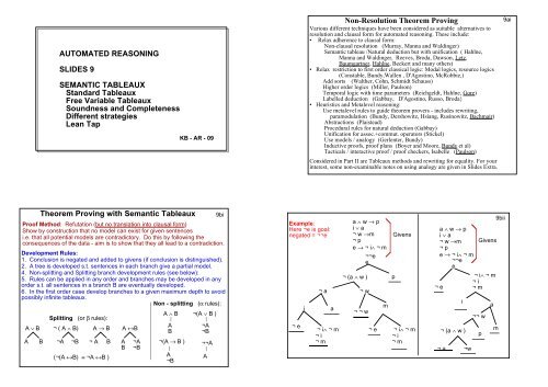
Theorem Proving with Semantic Tableaux
KB - AR - 09
Proof Method: Refutation (but no translation into clausal form)
Show by construction that no model can exist for given sentences
i.e. that all potential models are contradictory. Do this by following the
consequences of the data - aim is to show that they all lead to a contradiction.
Development Rules:
1. Conclusion is negated and added to givens (if conclusion is distinguished).
2. A tree is developed s.t. sentences in each branch give a partial model.
4. Non-splitting and Splitting branch development rules (see below):
5. Rules can be applied in any order and branches may be developed in any
order s.t. all sentences in a branch B are eventually developed.
6. In the first order case develop branches to a given maximum depth to avoid
possibly infinite tableaux.
Non - splitting (α rules):
A ∨ B
A B
Splitting (or β rules):
¬ ( A ∧ B)
¬A ¬B
A → B
¬ A B
(¬(A ↔B) ≡ ¬A ↔B )
A ↔B
A
B ¬A
¬B
A ∧ B
A
B
¬(A → B )
A
¬B
¬(A ∨ B )
¬A
¬B
¬¬A
A
9bi
Non-Resolution Theorem Proving
Various different techniques have been considered as suitable alternatives to
resolution and clausal form for automated reasoning. These include:
• Relax adherence to clausal form:
Non-clausal resolution (Murray, Manna and Waldinger)
Semantic tableau /Natural deduction but with unification ( Hahlne,
Manna and Waldinger, Reeves, Broda, Dawson, Letz,
Baumgartner, Hahlne, Beckert and many others)
• Relax restriction to first order classical logic: Modal logics, resource logics
(Constable, Bundy,Wallen , D'Agostino, McRobbie,)
Add sorts (Walther, Cohn, Schmidt Schauss)
Higher order logics (Miller, Paulson)
Temporal logic with time parameters (Reichgeldt, Hahlne, Gore)
Labelled deduction (Gabbay, D'Agostino, Russo, Broda}
• Heuristics and Metalevel reasoning:
Use metalevel rules to guide theorem provers - includes rewriting,
paramodulation (Bundy, Dershowitz, Hsiang, Rusinowitz, Bachmair)
Abstractions (Plaistead)
Procedural rules for natural deduction (Gabbay)
Unification for assoc.+commut. operators (Stickel)
Use models / analogy (Gerlenter, Bundy)
Inductive proofs, proof plans (Boyer and Moore, Bundy et al)
Tacticals / interactive proof / proof checkers, Isabelle (Paulson)
Considered in Part II are Tableaux methods and rewriting for equality. For your
interest, some non-examinable notes on using analogy are given in Slides Extra.
Example:
Here ¬e is goal:
negated = ¬¬e
¬ e
¬¬e
e
¬ (a ∧ w ) p
¬ a ¬ w
i a
¬ i∧ ¬ m
¬ i
¬ m
a ∧ w → p
i ∨ a
¬ w →m
¬ p
e → ¬ i∧ ¬ m
¬ ¬ w
m
Givens
¬ e ¬ i∧ ¬ m
¬ i
¬ m
a ∧ w → p
i ∨ a
¬ w →m
¬ p
¬ e
e → ¬ i∧ ¬ m
¬¬e
e
i
¬ (a ∧ w )
¬ a ¬w
Givens
¬ i∧ ¬ m
¬ i
¬ m
¬¬ w
p
a
m
9bii
9ai

What if the Givens do not imply the conclusion?
¬ e
a ∧ w → p
i ∨ a
¬ w →m
e → ¬ i∧ ¬ m
¬¬e
e
i
¬ (a ∧ w )
¬ i∧ ¬ m
¬ i
¬ m
¬¬ w
p
¬ a ¬w w
Givens
The invariant property SATISFY:
a
m
Example: Givens do not |= ¬e
There is a model of Givens and e
The branch ending in w does not close.
All data has been processed in the branch.
(It is called saturated.)
9biii
Since the assumption that a model of Givens
exists is not contradicted the branch is
consistent.
A model can be read from the literals in the
branch. Each atom that occurs positively will
be true in the model and each atom that
occurs negatively will be false. Other atoms
(that don't occur in the open branch) can be
true or false but are usually made false.
Here: a, e, p, w =True and i, m=False.
Note that no atom can occur both positively
and negatively in an open branch. Why?
• Each tableau extension rule maintains satisfiability:
if the sentences in a branch are satisfiable and a rule is applied, the new
sentences in at least one descendant branch are satisfiable.
e.g. If M is a model of a branch including i ∨ a, then M must assign true to at
least one of i or a. Hence at least one extended branch is satisfied by M.
• A branch that contains both X and ¬ X is unsatisfiable and can be closed
by the closure rule.
Quantifier rules (∀∀)) (γ rules) for Standard version (not often used now
except in proofs about tableau properties):
∀x P[x] ¬∃x P[x]
| |
P[t1] ¬ P[t1]
where t1 is a ground term from the
language.
e.g. ∀x P(x,f(x) )
⇒ P(s,f(s) )
In the standard version, each ∀ sentence in B should eventually be used for
every name that "occurs" in a sentence in B (unless the branch is closed). This
includes all names constructed from constants and functors in the branch
9bv
Semantic Tableaux
9biv
Semantic tableaux were introduced in 1954 by Beth. The standard method was automated in 1985,
when the free variable method was also automated. The Model Elimination approach was
introduced by both Kowalski and Loveland in 1970, but as a resolution refinement, not as a
tableau method. This was later related and extended to tableau methods in 1990 onwards. The
TABLEAUX Workshops (now part of IJCAR) are devoted to tableaux and related theorem
proving methods.
The initial branch of a semantic tableau contains the given sentences that are to be refuted.
Reasoning progresses by making assertions about the satisfiability of sub-formulas based on the
satisfiability of the larger formulas of which they are a part. The α-rules (slide 9bi) can be read as
"if α is in a branch and there is a model of the sentences in the branch, then there is a model of the
sentences in the branch extended by α1 and α2" and the β-rules as "if β is in a branch and there is a
model of the sentences in the branch, then there is a model of either the sentences in the branch
extended by β1, or the sentences in the branch extended by β2", where α1, α2/β1, β2 are the two
sub-formulae of the rules. If X and ¬X are in the branch then the sentences in the branch are clearly
inconsistent and the branch is closed. If all branches in a tableau are closed (it is also said to be
closed), then there are no possible consistent derivations of sub-formulas from the initially given
sentences, and these sentences are unsatisfiable.
Two examples of closed propositional tableaux are on slide 9bii, illustrating that there can be
differently sized tableaux for the same set of initial sentences. For propositional sentences the
development of a tableau will always terminate as there is no need to develop a sentence in a
branch more than once – to do so would duplicate one or more sub-formulas or atoms in that
branch, which adds no information to the branch. However, every sentence in a branch must be
developed in it. A fully developed (or completed) branch is called open if it is not closed, and
similarly the tableau . A fully developed open branch will yield a model of the initial data.
(1) div(x,x), (2) less(1,n), (3) div(u,w) ∧ div(w,z) → div(u,z) 9bvi
(4) ¬(div(g(x),x) ∧ less(1,g(x)) ∧ less(g(x),x) ) → pr(x)
(5) less(1,x)∧less(x,n)→div(f(x),x)∧pr(f(x)) Show ∃y (pr(y)∧div(y,n))
¬less(1,g(n)
¬∃y (pr(y)∧div(y,n)) (**) (Negated conclusion)
¬(pr(n) ∧div(n,n)) (guess n is a good value for y in (**) )
(4)
¬¬(div(g(n)n) ∧ less(1,g(n)) ∧ less(g(n),n))
div(g(n)n), less(1,g(n)), less(g(n),n)
¬(less(1,g(n)
∧ less(g(n),n))
¬less(g(n),n)
(5)
div(f(g(n)), g(n))
pr(f(g(n))
(**) ¬ (pr(f(g(n)) ∧div(f(g(n)),n))
¬pr(f(g(n))
(**) Guess f(g(n))
is a good value for y
¬ div(f(g(n)),n)
(Use (3) next)
¬pr(n)
pr(n)
¬div(n,n)
(1)
div(n,n)
A closed tableau using
the Standard γ rules:
1, n are constants;
all variables in data are
universally quantified.

Soundness and Completeness Statements for Tableaux:
9bvii
The soundness theorem for tableaux states that “if a set of sentences S is consistent,
then the tableau developed from S will not fully close”. Equivalently, "if the tableau
developed from sentences S closes, then S is inconsistent".
The completenss theorem for tableaux states that “if a set of sentences S is
unsatisfiable, then it is possible to find a fully closed tableau derived from them”.
The soundness theorem is a consequence of the property (SATISFY), which
guarantees that the development rules maintain consistency in at least one descendant
branch. Informally, therefore, if the original sentences are satisfiable, not all branches
can close. An outline proof of this property is on slide 9di.
First Order Tableaux (Standard Version)
There are two kinds of quantifier rules for tableaux; the standard rules for universaltype
quantifiers (either ∀ or ¬∃ ) are similar to the usual ∀−elimination rule for
natural deduction. That is, occurrences of the bound variable in the scope of the
quantifier may be replaced by any term in the language, including terms involving
other universally bound variables at the same outer level but in the scope of the
quantifier being eliminated. e.g.∀x∀y.P(x,y) could become ∀y.P(f(a),y) or even ∀y.
P(y,y). The problem with this form of the rule is that the substitutions have to be
guessed. (See example on 9bvi.) These rules are not often used in theorem provers
(although they may be used in proofs about tableau provers). Instead, free variable
rules are used instead. (Continued on 9cii.)
9ci
Free Variable Tableaux
In clausal reasoning resolution replaced guessing substitutions. Free variable
tableaux improve on standard tableaux by delaying γ rule substitutions.
Free variable γ rules
∀x P[x] ¬∃x P[x]
| |
P[x1] ¬ P[x1]
where x1 is a new free
variable in the tableau
Free variable δ rules
∃xP[x] ¬∀xP[x]
| |
P[a] ¬P[a]
e.g. ∀x P(x,f(x) ) ⇒ P(x1,f(x1) ) (x1 is new to tableau)
∃xP(x,a) ⇒ P(d,a)
∀y,w ∃xP(x,y,w) ⇒ ∃xP(x, y1,w1) ⇒ P(f(y1,w1), y1,w1)
where a is a term new to the
tableau dependent on the
free variables occurring
in ∀xP[x] or ∃xP[x]. (If no free
variables "a" is a constant.)
In a free variable tableau the CHOICE of substitution in a γ-rule application is
delayed until closure.
The closure rule causes free variables in the matching literals to be bound by
unification to achieve complementarity.
Wherever a free variable (x1 say) occurs in the tableau, it must be bound to
the same term (if it is bound at all).
Standard version
Quantifier rules (∃) (δ rules):
∃xP[x] ¬∀xP[x]
| |
P[a] ¬P[a]
where a is a new
constant symbol not
occurring in the
tableau (*) (also
called a parameter).
e.g. ∀y ∃xP(x,y,y)
⇒ ∃xP(x,b,b)
(b occurs in the tableau)
⇒ P(c,b,b)
(c is new to the branch)
(*) – in fact, the parameter only needs to be new to the branch).
It is often easier to Skolemise sentences before-hand (so existential-type
quantifiers in the data are eliminated (eg in 9bvi (4) g is a Skolem term).
Each ∃ sentence in a branch B is developed once in each branch below B
Often, ∀ expansion is combined
with some splitting rule and
possibly closure too.
The rules for A ∧/∨ B are
extended to deal with more than
one operator of the same kind.
Free Variable First Order Tableaux
¬ P(a)
∀x[P(x) ∨ Q(x)]
P(a) Q(a)
∀ + "∨" splitting +
closure +
choosing 'a' to
substitute for the
bound variable x.
9bviii
When free-variable rules are used for dealing with ∀ sentences, the substituted term is a
new variable, which acts like a place-holder until a suitable term can be decided. A global
binding environment for a tableau is maintained, which records eventual bindings to free
variables. This is analogous to the procedure in Prolog execution (which can, in fact, be
viewed as a particular free-variable tableaux development for Horn clauses).
Use of the free variable ∀ rule applied to ∀x∀y.P(x,y) yields P(x1, y1), where x1 and y1
are (fresh) free variables, and again there is the freedom for x1 to be bound to the same
term as y1. The occurs check is used when unifying at closure to prevent, for example, x1
subsequently being bound to f(x1), as this would lead to infinite terms.
Existential-type quantifiers are treated to a Skolemisation process - either at run-time
(similar to a natural deduction ∃-elimination rule), or before run-time (similar to the
Skolemisation step when converting to clausal form). Whereas for the standard rules the
process at run-time always results in a new constant being introduced, for the freevariable
rules it may result in a new (Skolem) function term whose arguments are the free
variables in the sentence in the scope of the ∃.
9cii

Show (1) - (5) |= ∃w. P(w)
(2) ∀y[Qxy → Rxg(y) ] → Px
(3) Sx → ¬Tg(x)f(y)
(4) (Txy → Rxy) → Kxy
(5) Qf(z)y ∧ Kzx → Rxg(y)
(1) Sa
(6) ∀w ¬Pw
(negated conclusion)
Variables in data
are universally
quantified.
a is a constant.
Work from L to R.
Free variable rules
Unify as you go
Px2
x2==w1
Rx3g(y3)
x3==w1
y3==h(w1)
Sa
9ciii
¬Pw1⇒¬Pf(z3) ⇒¬Pf(g(x4) ) ⇒ ¬Pf(g(a) )
Kx1y1
¬∀y[Qx2y → Rx2g(y)]
⇓
¬∀y[Qw1y → Rw1g(y)]
∃y[Qw1y ∧ ¬Rw1g(y)]
Qw1h(w1)
¬Rw1g(h(w1))
¬Qf(z3)y3
⇓
¬Qf(z3)h(w1)
w1==f(z3)
¬(Tx1y1 → Rx1y1)
⇓
¬(Tz3f(z3) → Rz3f(z3))
¬Kz3x3
⇓
¬Kz3w1
⇓
¬Kz3f(z3)
x1==z3
y1==f(z3)
Tz3f(z3)
¬Rz3f(z3)
¬Sx4
x4==a
¬Tg(x4)f(y4)
z3==g(x4)
y4==z3
Gives: {w1==f(g(a))==x2==x3==y1, x4==a, y3==h( f(g(a))), x1==g(a)==z3==y4}
Constructing Free Variable Tableaux
9cv
When constructing a free variable tableau, you may do it in one of two ways, which could be called
"unify as you go", or "unify at the end". The tableau on Slide 9ciii (as are all tableaux in Slides 9 -
11) is constructed using unify-as-you-go. In this kind of construction, whenever a closure is made
that requires a binding to be made to one or more free variables, the substitution is applied to all
occurrences in the tableau of those newly bound variables. This guarantees consistency of the
bindings as the tableau is constructed. Only one binding may be made to any free variable. The
propagation is shown on the slides by an arrow (⇒ or ⇓). In the example the tableau is developed
from left to right, although any order could have been followed. The unify-as-you-go approach is
useful for most applications, especially those using data structures, when it may be necessary for a
piece of data to be used many times. When applied to clauses, it has given rise to many different
refinements. See Slides 10 and 11.
In this kind of construction it can be shown that it is unnecessary to put two unconstrained
unbound variants of a universal sentence in a branch. However, as soon as such a variant is (even
partially) bound, then there is scope for a second variant. eg given ∀x[P(f(x)) ∨ Q(x)]; let P(f(x1))
be in a branch, then there is no need to use the sentence again as it would result in P(f(x2)), with
both x1 and x2 unbound. If later P(f(x1)) happened to be used in closure, binding x1 to a (say), then
sibling branches beneath P(f(x1))⇒P(f(a)) could use a second instance P(f(x2)), perhaps where the
binding of x2 is constrained to be different from a. This is analogous in not requiring development
of a ground sentence in a branch more than once.
The alternative method of unify-at-the-end is shown and discussed in Appendix 2. In this
construction, it is noted when a branch can close and what the corresponding binding is, but no
propagation takes place. When every branch has such a potential closure the possible substitutions
are combined (ie unified). If they do not unify then alternative closures in one or more branches are
sought. The approach is useful if it is known that one (or only a few) occurrences of a piece of data
will be needed. See Slide 9cvi for an example.
Developing Free Variable Tableaux
Method 1. unify-as-you-go (used in Slides 9 -11)
Unifiers are computed on closure and the resulting bindings are propagated
throughout the tableau (as on 9ciii).
The unifiers are always compatible at any stage of completion of the tableau.
Method 2. unify-at-the-end (See Appendix 2 and 9cvi).
Potential closures are marked, recording possible bindings to free variables.
When a potentially fully closed tableau has been found, a solution for all free
variables that satisfies one of the bindings at every closure is found.
The unify at the end approach is useful if it is known that one (or only a few)
occurrences of a piece of data will be needed. (See Appendix2.)
9civ
The unify-as-you-go approach is useful for most applications, especially those
using data structures, when it may be necessary for a piece of data to be used
many times. When it is applied to clauses, it has given rise to many different
refinements. See Slides 10 and 11.
(1) div(x,x), (2) less(1,n), (3) div(u,w) ∧ div(w,z) → div(u,z)
(4) ¬(div(g(x),x) ∧ less(1,g(x)) ∧ less(g(x),x) ) → pr(x)
(5) less(1,x)∧less(x,n)→div(f(x),x)∧pr(f(x)) Show ∃∃y (pr(y)∧div(y,n))
¬∃y (pr(y)∧div(y,n))
¬(pr(y1) ∧div(y1,n))
div(g(x1),x1) ∧ less(1,g(x1)) ∧ less(g(x1),x1)
¬ less(1,x2)
x2==g(x1)
¬ less(x2,n)
x2==g(x1)
x1==n
(or x2==1 is
possible)
div(f(x2), x2)
pr(f(x2))
¬ (pr(y2)) ∧div(y2,n))
div(u1,z1)
¬ div(u1,w1)
u1==f(x2)
w1==x2
¬div(w1,z1)
z1==x1
w1=g(x1)
¬ pr(y2)
y2==f(x2)
pr(x1)
¬ pr(y1) ¬ div(y1,n)
y1==x1
Gives: { x2==w1==g(n), x1==y1==x3==z1==n, u1==y2==f(g(n))}
Free variable rules
Unify at the end
div(x3,x3)
¬ div(y2,n)
y2==u1,
z1==n
y1==n
x3==n
9cvi

Benefits of the Tableau Approach
• Uses the original structure of knowledge - no need to convert to clausal
form and so no exponential expansion in presence of ↔ sentences;
• Extends to non-classical logics very easily - most non-classical automated
techniques use tableaux as they can mimic the semantics closely;
• Lends itself to linear reasoning - at each extension step made to a leaf L
use a sentence that closes one branch using L.
eg Logic Programming can be seen as tableau development;
• Can incorporate equality - we will see later how tableau incorporate
equality quite naturally.
9cvii
• Free variable tableaux may terminate without closure for satisfiable
sentences, even when standard tableaux would be infinite (but still unclosed);
• Free variable tableau for clausal data are like extensions to Prolog; there are
many refinements, often derived from resolution refinements.
In Slides 10 we'll look at Model Elimination, the basis for many of them.
Proof of Soundness of Tableau:
The tableau soundness proof relies on the SATISFY property on Slide 9biv. The cases
for boolean operators are all simple and similar to the case given on Slide 9di.
For the standard ∀ case, the argument on 9di is justified as follows. As in resolution, it
is simplest to assume the domain is non-empty (else there are complications). Therefore,
assume the domain of M is non-empty. The assignment for t will either already be made
in M, or, if t is new and no assignment for t is yet made in M, then t can be any domain
element. Either way M will remain a model since, in M, P[x] is true for every x in the
domain.
In case x is captured by another universal quantifier, as in ∀x,u. P(x,u) becoming
∀u.P(u,u), then since ∀u. P(x,u) is true in M for every domain element substituted for x,
it is the case that for each domain element substituted for x, P(x,x) is true in M, which is
what ∀u P(u,u) is true means.
For the standard ∃ case, one can either include in the signature additional parameters to
be used as needed (and which are similar to Skolem constants), or introduce new names
as the need arises. In both cases it is assumed that M does not have an assignment for the
name t introduced by the rule. Since ∃x.P[x] is true, P[a] must be true for some element a
in the domain of M. The assignment for the new name t can be the witness a.
The cases for the free variable rules are considered on 9dvii.
9dii
Standard Tableaux:
The Tableau Method is Sound
A closed tableau for S implies that S is unsatisfiable
• First show that each tableau extension rule maintains SATISFY:
if the sentences in a branch are satisfiable and a rule is applied,
then the new sentences in at least one descendant branch are satisfiable.
• eg: the rule for →: If A → B is in a branch X and there is a model for the
sentences in X, then this model at least makes A false or B true. Hence the same
model will ensure satisfiability in one of the two extension branches.
• eg: the rule for ∀: Suppose ∀x P[x] occurs in a branch B and M is a model for
sentences in B. Then if P[t] is added and t is aready interpreted in M then M is
still a model; otherwise, M can be extended by interpreting t as some domain
element and still remain a model. (If data is Skolemised at the start then Sig(S) is
known and the first case always applies.)
• Other cases are similar (see 9dii).
• (SATISFY) implies that satisfiable initial sentences can never lead to a fully
closed tableau, as there is always a branch with a model which must be open.
(Formally use an induction argument on depth of the tableau.)
• Therefore a fully closed tableau indicates unsatisfiability of the initial sentences.
To formalise the proof showing a fully closed tableau implies that a set of 9diii
sentences S is unsatisfiable we use induction on the depth of a tableau to show (**)
If S is a satisfiable set of sentences then,
forall n≥≥0, if a tableau of depth n is developed from S
then that tableau has at least one satisfiable and open branch.
The depth of a tableau is the maximum number of non-closure rule applications in any
branch.
Assume that S is satisfiable.
Base Case: (n = 0); Since S is satisfiable there is a model for S. In particular there
cannot be a sentence and its negation so the initial branch is open, and satisfiable.
Induction Step (n>0). Let there be a tableau of depth n developed from S called T.
Assume as induction hypothesis (IH) that for a satisfiable set of sentences S,
forall 0≤k

Using Standard Rules:
The tableau method is Complete
For unsatisfiable S a closed tableau for S exists.
• Apply rules (possibly by contemplating rule applications for an "infinite"
number of times) to obtain a maximally developed (saturated) tableau, in
which all possible applications of the α, β, δ rules are made in all branches
and all instances of ∀ sentences are added to each appropriate branch.
eg if p ∧ q is in a branch B then both p and q are also in B
9div
• If such a maximal tableau doesn't close, then at least one branch B is open
and a model of the sentences in B can be found, based on the individual
literals occurring in B. (See slides 9dv and 9dvi.)
• A H-interpretation is constructed using as domain the terms built from
symbols occurring in sentences in B, such that atoms in B are assigned true
and all other atoms are assigned false.
• Hence if the initial sentences are unsatisfiable they must lead to a closed
tableau.
The case for Free variable rules is on Slide 9dvii.
Constructing a Model from an open branch in a Saturated Tableau
• Suppose a standard tableau has been fully developed from initial
sentences S, as described on Slide 9div, and that there is an open branch B.
• Let T be the set of sentences in B and M be a first order H-interpretation of
T with domain terms built from symbols in T and constructed as follows:
Each atom in T is true in M; all other atoms are false in M.
• We show M is a model of T.
• Suppose not: then some sentence in T is false in M.
• Let X be the smallest sized sentence in T s.t. M makes X false.
• Whatever type of sentence X is, its being false leads to a contradiction:
• X cannot be an atom, by construction.
• eg: case X is ¬ Y (Y atom) : If ¬Y is false in M, then Y is true. But then Y
occurs in T and closure would have occurred.
• eg: case X is A ∨ B : If A ∨ B is false in M then both A and B are false in M
and smaller than A ∨ B; but at least one of A or B is in T, contradicting that X
is the smallest false sentence in T.
• eg: case X is ∀xP[x] : If ∀xP[x] is false in M then P[t] is false for some
domain element t. But by construction P[t] occurs in T and is smaller than
∀xP[x] (assume size is depth of parse tree of X).
• Other cases are similar.
9dvi
Example of a Saturated Tableau
Given: b(c) ∃y.on(c,y) ¬b(x)∨¬g(x) ¬on(x,z)∨g(x)∨ ¬g(z)
(Variables x,z are universally quantified)
∃y.on(c,y)
b(c)
on(c,d)
¬b(c) ¬g(c)
¬on(c,d)
g(c)
Extensions by any other
instances (4 possibilities in all)
duplicate at least one literal in
the remaining open branch. Such
extensions are unnecessary.
Exercise: Check this is true.
Soundness:
¬g(d)
• Domain of H-model in the open
branch = {c,d}
• The atoms are on(c,d), b(c), so
these are True.
• All other atoms are false:
on(c,c), on(d,d), on(d,c), b(d), g(c),
g(d).
9dv
Check:
• Clearly b(c) and ∃y.on(c,d) are true.
• For each x, g(x) is false so
¬b(x)∨¬g(x) is true.
• For z = c, ¬on(x,z)∨g(x)∨ ¬g(z) is
true as g(c) is false.
• Similarly for z=d.
Soundness and Completeness of free variable tableau
When a free variable tableau closes, there may be free variables in it not yet
bound. These can be bound (consistently) to any ground term yielding a
ground tableau, which will still close. Then use Soundness of a standard
tableau.
Completeness (outline):
A closed standard tableau may be lifted to a tableau using free variables:
Each use of the standard ∀-rule is made into a use of the γ -rule, with a fresh
set of variables, and each closure then becomes one or more equations to be
solved by unification.
Since the tableau is closed, a unifier satisfying the set of equations derived in
this way exists and hence a most general unifier (mgu) exists also.
This mgu can be obtained by the unification algorithm in one attempt ("unify at
the end") or in a distributed attempt, corresponding to the different branch
closures ("unify as you go"). 9dvii

LeanTap: A Free Variable Tableau Theorem Prover 9ei
%prove(currentFormula,todo,branchLits,freevars,maxvars)
%Conjunction case (alpha rule)
prove((A,B),UE,Ls,FV,V) :- !, prove(A,[B|UE],Ls,FV,V).
%Disjunction case - split (beta rule)
prove((A;B),UE,Ls,FV,V) :- !, prove(A,UE,Ls,FV,V),
prove(B,UE,Ls,FV,V).
%Universal case - keep data all(X,Fm)
prove(all(X,Fm),UE,Ls,FV,V) :- !,
\+ length(FV,V),copy_term((X,Fm,FV),(X1,Fm1,FV)),
append(UE,[all(X,Fm)],UE1),
prove(Fm1,UE1,Ls,[X1|FV],V).
%Closure case
prove(Lit,_,[L|Ls],_,_) :-
(Lit = -Neg; -Lit = Neg) ->
(unify_with_occurs_check(Neg,L); prove(Lit,[],Ls,_,_)).
%Literal not matching case
prove(Lit,[N|UE],Ls,FV,V) :-prove(N,UE,[Lit|Ls],FV,V).
Formulas are in Skolemised negated normal form (negations next to atoms).
nnf(-(-(p=>q)=>(q=>p)), ((p,-q),(q,-p)))
nnf(-(((p=>q)=>p)=>p), (((p,-q);p),-p))
nnf(ex(Y,all(X,(f(Y)=>f(X)))), all(X,(-f(s);f(X))))
(The code generates all(X,(f(Y)=>f(X))) as Skolem term s)
Example queries to run:
F= (-h(a), all(X,(f(X);h(X))),all(Z,(-g(Z);-f(b))),
all(Y,(-f(Y);-h(b))),all(X,(g(X);-f(X)))),
prove(F,[],[],[],4)
nnf(-(-e)&(a & w =>p)&(i v a)& -p&(e =>-i & -m)&(-w =>m), F),
prove(F,[],[],0)
1. Add write instructions so that information about the structure of the tableau is printed
out, including closure.
2. Explain details of universal and closure cases of prove and existential case of nnf.
3. Run other examples covered in slides and exercises.
What improvements could be made?
a) add a loop check. (Note that (for example) h(X) and h(Y) do not form a loop - so must
be careful to match terms identically.
b) add a higher level predicate prove1 that calls prove recursively, each time increasing
the freevars limit by 1.
c) limit the depth of each branch instead of the number of freevars.
9eiii
:- op(400,fy,-),op(500,xfy,&),op(600,xfy,v),
op(650,xfy,=>), op(700,xfy,).
nnf(Fml,NNF) :- nnf(Fml,[],NNF).
nnf(Fm,FV,NNF) :-
(Fm = -(-A) -> Fm1 = A;
Fm = -all(X,F) -> Fm1 = ex(X,-F);
Fm = -ex(X,F) -> Fm1 = all(X,-F);
Fm = -(A v B) -> Fm1 = -A & -B;
Fm = -(A & B) -> Fm1 = -A v -B;
Fm = (A => B) -> Fm1 = -A v B;
Fm = -(A => B) -> Fm1 = A & -B;
Fm = (A B) -> Fm1 = (A & B) v (-A & -B);
Fm = -(A B) -> Fm1 = (A & -B) v (-A & B)),!,
nnf(Fm1,FV,NNF).
nnf(all(X,F),FV,all(X,NNF)) :- !, nnf(F,[X|FV],NNF).
nnf(ex(X,Fm),FV,NNF) :- !,
copy_term((X,Fm,FV),(Fm,Fm1,FV)), nnf(Fm1,FV,NNF).
nnf(A & B,FV,(NNF1,NNF2)) :- !,
nnf(A,FV,NNF1), nnf(B,FV,NNF2).
nnf(A v B,FV,(NNF1;NNF2)) :- !,
nnf(A,FV,NNF1),nnf(B,FV,NNF2).
nnf(Lit,_,Lit). 9eii
LeanTap Prover
The LeanTap theorem prover was developed by Bernard Beckert, Joachim Possega
and Reiner Hahlne. It was the first ``Lean'' theorem prover, meaning a ``very small
Prolog program'' that exploits Prolog unification in clever ways to implement a
theorem prover for first order logic. A different, but equally good, prover is given on
Slides 10. It is called LeanCop. There was a whole culture built around Lean provers,
with people trying to outdo each other with their clever constructions. It is always
impressive to see how compact a theorem prover in Prolog can be.
For simplicity, LeanTap uses formulas in Skolemised Negation Normal Form
(NNF). This means that before trying to develop a tableau existential type quantifiers
are replaced by Skolem functions and negations are pushed inwards so they are next
to atoms; however, no distribution of ∧ over ∨, or ∨ over ∧, is applied. This sentence
structure allows to simplify the top level of LeanTap, so only conjunctions and
disjunctions, universal quantifers and literals need be considered. (LeanCop uses
clausal form, which is a sub-case of NNF – ie distribution of ∨ over ∧ is performed.
Closure is checked for literals only. The Skolemisation step in `nnf' uses the name of
the formula being Skolemised as the new Skolem constant.
There are several websites covering LeanTap - just type it into Google and see!
9ev

Summary of Slides 9
1. Semantic Tableau methods provide an alternative to resolution for theorem
proving. They are also based on refutation and for a given set of sentences S
attempt to demonstrate that S can have no models.
2. In the ``standard'' tableau method, rules for dealing with universal (∀)
sentences require substitution of ground terms for the bound variable. In the
``free variable'' tableau method fresh variables are substituted, which can be
bound on branch closure using unification.
3. In the ``unify-as-you-go'' development strategy the bindings of free variables
are immediately propagated to all occurrences of the variables in the tableau. In
the ``unify-at-the-end'' development strategy potential bindings for free variables
are recorded and on (potential) closure of all branches in the tableau they are
combined. In effect, the difference between the two strategies is whether to
combine unifiers as they are generated, or to wait until all have been generated.
4.The tableau method is sound and complete. The free variable soundness and
completeness properties are derived from those of the standard tableau method.
5. The soundness property of tableau depends on the SATISFY property, which
states that, for a consistent branch, the tableau rules maintain consistency in at
least one descendant branch.
9fi
6. The completeness property depends on the notion of saturation, the 9fii
development of a tableau to include all possible applications of each rule in
every branch.
7. There are several implementations of the tableau method. The LeanTap
approach uses Prolog and results in a very compact program. It exploits
Prolog's use of variables to implement the unfication and propagation of free
variables.
8. The tableau method has several benefits, including: it uses the original
structure of the data, can be extended to many logics such as modal/temporal
logic, can easily incorporate equality, and linear and many other refinements
can be defined for the tableau method.
9. If a tableau terminates finitely without closing every branch, then a model
can be found for any remaining open branches (a possibly different one for
each open branch). The slides showed how to construct the model for
standard tableaux. It is also possible to do so for free variable tableaux.
(Exercise: Show how to do this for clausal data. It relies on a termination
condition that prevents more than one occurrence of any literal in a branch, in
which the free variables are still unconstrained. e.g. if the literal P(x,y) occurs
in a clause and P(x1,y1), derived from this literal is in a branch, then there is
no need for P(x2,y2) unless x1 or y1 have been constrained.)