Full document: PDF - Profs.info.uaic.ro - Universitatea Alexandru ...
Full document: PDF - Profs.info.uaic.ro - Universitatea Alexandru ...
Full document: PDF - Profs.info.uaic.ro - Universitatea Alexandru ...

Create successful ePaper yourself
Turn your PDF publications into a flip-book with our unique Google optimized e-Paper software.
T<br />
E<br />
C<br />
H<br />
N<br />
I<br />
C<br />
A<br />
L<br />
R<br />
E<br />
P<br />
O<br />
R<br />
T<br />
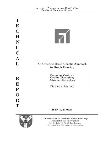
University “<strong>Alexandru</strong> Ioan Cuza” of Ia¸si<br />
Faculty of Computer Science<br />
An Ordering-Based Genetic App<strong>ro</strong>ach<br />
to Graph Coloring<br />
Cornelius C<strong>ro</strong>itoru<br />
Ovidiu Gheorghie¸s<br />
Adriana Gheorghie¸s<br />
TR 05-03, July 2005<br />
ISSN 1224-9327<br />
<strong>Universitatea</strong> “<strong>Alexandru</strong> Ioan Cuza” Ia¸si<br />
Facultatea de Informatică<br />
Str. Berthelot 16, 700483 -Ia¸si, Romania<br />
Tel. +40-232-201090, email: bibl@<st<strong>ro</strong>ng>info</st<strong>ro</strong>ng>iasi.<strong>ro</strong>
An Ordering-Based Genetic App<strong>ro</strong>ach to Graph<br />
Coloring<br />
Cornelius C<strong>ro</strong>itoru, Ovidiu Gheorghie¸s, and Adriana Gheorghie¸s<br />
University “Al. I. Cuza” Ia¸si, Romania<br />
Faculty of Computer Science<br />
{c<strong>ro</strong>itoru,ogh,adrianaa}@<st<strong>ro</strong>ng>info</st<strong>ro</strong>ng>iasi.<strong>ro</strong><br />
Abstract. We int<strong>ro</strong>duce a new evolutionary formulation of the graph<br />
coloring p<strong>ro</strong>blem, based on the interplay between orderings and colorings<br />
of vertices. The new formulation aims at breaking the symmetry in<br />
the solution space and p<strong>ro</strong>vides opportunities for combining evolutionary<br />
and other search techniques. Our formulation is very simple compared<br />
to previous app<strong>ro</strong>aches which use the relationship between a graph’s<br />
ch<strong>ro</strong>matic number and its acyclic orientations. We have experimented<br />
on graphs f<strong>ro</strong>m the DIMACS Computational Challenge. The results p<strong>ro</strong>vide<br />
evidence that the ordering app<strong>ro</strong>ach can be used to obtain accurate<br />
colorings. We also give a general p<strong>ro</strong>perty which accounts for the computational<br />
difficulty of all app<strong>ro</strong>aches that attempt to iteratively reduce<br />
the number of colors in a coloring.<br />
1 Int<strong>ro</strong>duction<br />
If G = (V,E) is a graph and k a positive integer, a k-coloring of (the vertices<br />
of) G is any assignment c : V → {1,..,k} with the p<strong>ro</strong>perty that for each<br />
i ∈ {1,...,k} the set c −1 (i) = {v|v ∈ V,c(v) = i} is a stable set in G, that is a<br />
set of mutually non-neighbor vertices. The set c −1 (i) is called the color class i of<br />
the coloring c and the list (S1,...,Sk) of all color classes completely determines<br />
the coloring c.<br />
It is well-known that it is NP-complete to decide whether, for a given graph<br />
G and an integer k there exists a k-coloring of G [10], [15]. The least possible<br />
number k of colors for which a graph G has a k-coloring is called the ch<strong>ro</strong>matic<br />
number of G and is denoted by χ(G).<br />
The graph coloring p<strong>ro</strong>blem is the p<strong>ro</strong>blem of finding, for a given graph G, an<br />
optimal coloring, that is a coloring with χ(G) colors. Since this p<strong>ro</strong>blem is not<br />
app<strong>ro</strong>ximable within |G| 1/14−ǫ for any ǫ > 0 [4], the graph coloring p<strong>ro</strong>blem is<br />
one of the favorites to try new meta-heuristics for (e.g. simulated annealing [14],<br />
tabu search [13]). Other app<strong>ro</strong>aches include DSatur [5] and greedy strategies [6]<br />
which have been outperformed by hybrid techniques based on maximal stable<br />
sets [9].<br />
We p<strong>ro</strong>vide a new evolutionary formulation of the graph coloring p<strong>ro</strong>blem<br />
which is based on the interplay between orderings and colorings of the vertices.<br />
This formulation gives the possibility of combining evolutionary and other search
2 Cornelius C<strong>ro</strong>itoru, Ovidiu Gheorghie¸s, and Adriana Gheorghie¸s<br />
techniques. We note that our formulation is very simple compared with that<br />
given in [3] which uses the well-known relationship that exists between a graph’s<br />
ch<strong>ro</strong>matic number and its acyclic orientations [8].<br />
We also give a general p<strong>ro</strong>perty that shows how a k − 1 coloring can be obtained<br />
form an already constructed k coloring. This p<strong>ro</strong>perty is used to devise a<br />
graph coloring algorithm. The p<strong>ro</strong>perty can also be used to explain the computational<br />
difficulty of all app<strong>ro</strong>aches that attempt to iteratively reduce the number<br />
of colors in a coloring, thus leaving open the quest for yet more powerful techniques.<br />
However, the “no free lunch” theorem ([19], [20], [7]) states that there<br />
cannot be a single algorithm that prevails over others for all p<strong>ro</strong>blem instances.<br />
2 Orderings and Colorings<br />
Let G = (V,E) be a graph with the vertices set V = {1,2,...,n}. The set of all<br />
n! permutations on the set V is denoted by Sn and each permutation v ∈ Sn,<br />
v = v1v2...vn, is interpreted as an ordering of vertices of G: v1 is the first vertex<br />
in the ordering v, v2 is the second one and so on.<br />
For vi ...vj ∈ Sn and i,j ∈ {1,...,n}, i < j we denote by I[v,i,j] the interval<br />
determined by the two indices i and j in v, that is, I[v,i, j] = {vi+1,...,vj−1}.<br />
We also denote by G[v,i, j] the subgraph induced in G by I[v,i, j].<br />
Definition 1. Let e ∈ E be an edge of G and v ∈ Sn an ordering. We call e a<br />
bad edge with respect to v if e = vivj, i < j and G[v,i, j] − e is a null subgraph<br />
of G.<br />
Note that by this definition any edge connecting two consecutive vertices in<br />
v, e = vivi+1, is a bad edge with respect to v.<br />
For each ordering v ∈ Sn we denote by b(v) the number of all bad edges in<br />
G with respect to v.<br />
The following theorem and its p<strong>ro</strong>of show that determining an optimal coloring<br />
in a graph is equivalent to finding an ordering of its vertices with a minimum<br />
number of bad edges.<br />
Theorem 1.<br />
χ(G) = 1 + min b(v)<br />
v∈Sn<br />
P<strong>ro</strong>of. 1. Let v 0 ∈ Sn be an ordering with minimum number of bad edges.<br />
Starting with v0 1 construct a maximal stable set of consecutive vertices in v0 :<br />
{v0 1,...,v 0 i }. Clearly, i ≥ 1 and either i + 1 > n or v0 i+1 is adjacent with at<br />
least one vertex f<strong>ro</strong>m {v0 1,...,v 0 i }. Call this stable set S1 and repeat the above<br />
construction, starting with v0 i+1 and obtaining S2,S3,..., until all vertices of<br />
v0 have been considered. We obtain a k-coloring (S1,S2,...,Sk) of G with the<br />
p<strong>ro</strong>perty that for each t ∈ 2,...,k, if v0 j is the first vertex (with respect to the
An Ordering-Based Genetic App<strong>ro</strong>ach to Graph Coloring 3<br />
ordering v0 ) of St, then there is a last vertex v0 i in St−1 such that v0 i v0 j ∈ E.<br />
Clearly, by the choice of v0 i , the edge v0 i v0 j is a bad edge with respect to v0 . Thus,<br />
the number k of colors in the coloring associated with v0 satisfies the inequality<br />
k − 1 ≤ b(v0 ). Since k ≥ χ(G), we have<br />
χ(G) ≤ k ≤ 1 + b(v 0 ) (1)<br />
2. Let (S1,S2,...,Sk) be an optimal (k = χ(G)) coloring of G. Each stable set<br />
Si, 1 ≤ i ≤ k−1 can<br />
<br />
be extended<br />
<br />
to become a maximal stable set in the subgraph<br />
induced in G by Si Si+1 ... Sk. The number of stable sets obtained remains<br />
k since k = χ(G). The obtained k-coloring (S1,S2,...,Sk) has the p<strong>ro</strong>perty that<br />
each vertex u ∈ Si has at least one neighbor in Si−1, 2 ≤ i ≤ k. Using this<br />
p<strong>ro</strong>perty we construct an associated ordering v0 ∈ Sn in the following way:<br />
(a) the last vertices in the ordering v 0 are the vertices of Sk in an arbitrary<br />
order; if Sk = {s1,...,sp} then v 0 n = s1, v 0 n−1 = s2,...,v 0 n−p+1 = sp;<br />
(b) the vertex before v 0 n−p+1 (i.e. v 0 n−p) is a vertex u ∈ Sk−1 which is a neighbor<br />
of v 0 n−p+1; there is such a vertex by the above p<strong>ro</strong>perty of the coloring.<br />
Put vn−p = u and the remaining vertices of Sk−1 are added to v 0 in an<br />
arbitrary order (i.e. Sk−1 − {u} = {u1,...,ut}, put v 0 n−p−1 = u1, v 0 n−p−2 =<br />
u2,...,v 0 n−p−t = ut);<br />
(c) repeat (b) for Sk−2,Sk−3,... until all vertices of S1 (and therefore of G) are<br />
added to v 0 .<br />
The ordering v0 constructed above has only k − 1 bad edges, namely those<br />
obtained in the step (b) of the algorithm, connecting consecutive vertices in v0 which have also consecutive colors. Therefore we have b(v0 )+1 = k = χ(G) and<br />
since b(v0 ) ≥ minv∈Sn b(v) we obtain<br />
χ(G) = b(v 0 ) + 1 ≥ 1 + min b(v) (2)<br />
v∈Sn<br />
By (1) and (2) the theorem holds. ⊓⊔<br />
Let us note that by (1) and (2) above the coloring and the ordering constructed<br />
in the p<strong>ro</strong>of are optimal. In other words, the two constructions described<br />
in the p<strong>ro</strong>of show how to efficiently obtain an optimal coloring f<strong>ro</strong>m an ordering<br />
with minimum number of bad edges and conversely.<br />
3 Description of the Genetic Algorithm<br />
This section describes a genetic algorithm which employs ordering based app<strong>ro</strong>ach<br />
to graph coloring.<br />
Genetic algorithms [16] are p<strong>ro</strong>babilistic techniques which mimic the natural<br />
evolutionary p<strong>ro</strong>cess. A genetic algorithm maintains a population of candidate<br />
solutions. This is one important feature that differentiates them f<strong>ro</strong>m conventional<br />
heuristics like hill climbing, simulated annealing, tabu search etc. Genetic
4 Cornelius C<strong>ro</strong>itoru, Ovidiu Gheorghie¸s, and Adriana Gheorghie¸s<br />
algorithms have thus the potential to better explore the search space; moreover,<br />
they p<strong>ro</strong>vide tools for avoiding “premature convergence”.<br />
Each candidate solution in the population is encoded into a structure called<br />
ch<strong>ro</strong>mosome. To each ch<strong>ro</strong>mosome, a value (called fitness value) is assigned. The<br />
fitness value represents the quality of the candidate solution encoded by the<br />
ch<strong>ro</strong>mosome. Assigning fitness values to ch<strong>ro</strong>mosomes is called evaluation.<br />
A selection p<strong>ro</strong>cedure simulates the “survival of the fittest” paradigm f<strong>ro</strong>m<br />
nature. Better-fitted ch<strong>ro</strong>mosomes have higher chances of surviving to the next<br />
generation. The number of ch<strong>ro</strong>mosomes per generation is constant.<br />
As in natural life, offspring ch<strong>ro</strong>mosomes are obtained f<strong>ro</strong>m parent ch<strong>ro</strong>mosomes.<br />
One possibility is for two parents to exchange encoded <st<strong>ro</strong>ng>info</st<strong>ro</strong>ng>rmation and<br />
thus creating two new offspring; this is called c<strong>ro</strong>ssover. Another possibility is to<br />
alter the encoded <st<strong>ro</strong>ng>info</st<strong>ro</strong>ng>rmation in a ch<strong>ro</strong>mosome obtaining a slightly different new<br />
ch<strong>ro</strong>mosome; this is called mutation. Some other ch<strong>ro</strong>mosomes simply survive<br />
unaltered, while others die off. Mutation and c<strong>ro</strong>ssover are referred to as genetic<br />
operators.<br />
3.1 Representation<br />
A ch<strong>ro</strong>mosome represents an ordering of the vertices of the graph. We encode<br />
the ordering by means of a permutation.<br />
If the graph has n vertices, the ch<strong>ro</strong>mosome will be a vector<br />
ch<strong>ro</strong>m = (v1,v2,...,vn), where vi ∈ {1,2,...,n}, vi = vj,i = j (3)<br />
The candidate solution represented by the ch<strong>ro</strong>mosome is obtained in a<br />
straightforward manner: the position of vertex vi in the ordering is i.<br />
3.2 Evaluation<br />
The purpose of evaluation is to point out how good the candidate solution encoded<br />
by a ch<strong>ro</strong>mosome is. In order to p<strong>ro</strong>vide such a measurement, a coloring<br />
is constructed f<strong>ro</strong>m each ordering (ch<strong>ro</strong>mosome). The number of colors of the<br />
coloring (or, alternatively, the number of bad edges) is taken as a measure of an<br />
individual’s quality. This is consistent with the minimization of the number of<br />
colors.<br />
Typically, a heuristic for graph coloring consists of two parts: in the first<br />
part, a suitable ordering of the vertices is fixed and in the second part, the<br />
actual coloring algorithm is applied using the fixed order of vertices. A very<br />
basic coloring p<strong>ro</strong>cedure is the sequential algorithm (sometimes called greedy<br />
algorithm), which p<strong>ro</strong>ceeds as follows. Assume the vertices of the graph are given<br />
in the order v1,v2,...,vn; they will be p<strong>ro</strong>cessed in this order. Assign color 1 to<br />
v1. For each of the remaining vertices vi, assign to vi the minimum color number<br />
available, that is, the smallest color number that, so far, has not been assigned<br />
to any vertex adjacent to vi. Though the local action of the sequential algorithm<br />
appears to be quite reasonable, globally it may fail miserably for unfavorable
An Ordering-Based Genetic App<strong>ro</strong>ach to Graph Coloring 5<br />
vertex orderings. It is not difficult to construct a sequence G3,...,Gm,... of graphs<br />
such that each Gm is 2-colorable, the size of Gm is linear in m, and yet the<br />
number of colors used by the sequential algorithm on input Gm is at least m for<br />
at least one vertex ordering.<br />
Similar results can be obtained for other graph coloring heuristics, most of<br />
which apply the sequential coloring algorithm to various vertex orderings that<br />
are obtained by seemingly reasonable p<strong>ro</strong>cedures.<br />
Furthermore, these computational results conducted us to a novel app<strong>ro</strong>ach<br />
to the above sequential p<strong>ro</strong>cedure (we call it LexBF). Clearly, the sequential<br />
coloring can be equivalently implemented by finding successive lexicographic-first<br />
maximal stable sets with respect to a previously fixed ordering v1,v2,...,vn, until<br />
all vertices are considered. If the order of the remaining vertices is changed after<br />
each construction of a color class it seems that this adaptive coloring algorithm<br />
p<strong>ro</strong>ceeds better. A good candidate for a dynamic changing of the ordering can<br />
be deduced f<strong>ro</strong>m the following interesting observation.<br />
P<strong>ro</strong>position 1. Let G = (V,E) be a graph and w1,w2,...,wn a vertex ordering<br />
generated by a breadth first traversal of G. If S is the lexicographic-first (with<br />
respect to the BFS ordering w1,w2,...,wn) maximal stable set of G, then the<br />
bipartite graph obtained f<strong>ro</strong>m G by deleting all edges with both extremities in<br />
V − S, has the same connected components as the graph G.<br />
Indeed, we can suppose that G is connected and it is not difficult to show<br />
that any vertex v of G can be reached f<strong>ro</strong>m the vertex w1 on a path that uses<br />
edges with only one extremity in V −S (by induction on the distance in G f<strong>ro</strong>m<br />
v to w1). The maximal stable set S has, by the above p<strong>ro</strong>position, the p<strong>ro</strong>perty<br />
that it is incident to many edges (at least n−1, if G is connected) in a somewhat<br />
uniform way. We note that there are nondeterministic choices to be made whenever<br />
there are more neighbors not yet visited at any point in the BF traversal<br />
of G. These ties will be solved by using an initial ordering v1,v2,...,vn. Our new<br />
graph coloring heuristic can be described as:<br />
Use a particular ordering v1,v2,...,vn to direct all the BF traversals<br />
While G is not empty do<br />
Apply a BF traversal to G and find the first<br />
(in the lexicographic BF ordering obtained) maximal stable set S;<br />
Let S be the new color class;<br />
G:=G-S<br />
Experimental results show that the LexBF heuristic performs better than the<br />
sequential algorithm (table 1). For this reason we have used LexBF as fitness<br />
function for the genetic algorithm.
6 Cornelius C<strong>ro</strong>itoru, Ovidiu Gheorghie¸s, and Adriana Gheorghie¸s<br />
3.3 Genetic Operators<br />
The <strong>ro</strong>le of the genetic operators ([12], [17]) is to explore the search space and<br />
to exploit the <st<strong>ro</strong>ng>info</st<strong>ro</strong>ng>rmation acquired during the evolution p<strong>ro</strong>cess. Each operator<br />
has a rate, which results in the number of ch<strong>ro</strong>mosomes to which that operator<br />
is applied. These rates are parameters of the genetic algorithm; they are tuned<br />
in order to balance exploration and exploitation [2].<br />
Guiding the search of the genetic algorithm towards p<strong>ro</strong>mising regions in<br />
the search space requires additional knowledge about the p<strong>ro</strong>blem to be incorporated.<br />
Valuable <st<strong>ro</strong>ng>info</st<strong>ro</strong>ng>rmation is p<strong>ro</strong>vided by the fitness function because color<br />
classes are constructed in a deterministic way. Early choices influence subsequent<br />
options. This means that preserving the relative order of some vertices may preserve<br />
the structure of a particular color class. Also, changing the relative order<br />
of vertices may induce changes in the color classes.<br />
We define one c<strong>ro</strong>ssover operator and three mutation operators. They are<br />
designed to either preserve a relative ordering of some vertices (c<strong>ro</strong>ssover), or<br />
modify it (mutations).<br />
C<strong>ro</strong>ssover The c<strong>ro</strong>ssover is designed to p<strong>ro</strong>pagate and exchange <st<strong>ro</strong>ng>info</st<strong>ro</strong>ng>rmation<br />
regarding color classes th<strong>ro</strong>ughout evolution. Since color classes are supposedly<br />
built f<strong>ro</strong>m successive nodes in parent ch<strong>ro</strong>mosomes, there are blocks of nodes<br />
which are inherited by offspring. There is no a priori reason for such blocks<br />
to have the same size, which leads to the idea of using two possibly different<br />
cutpoints, one for each parent.<br />
Let parent 1 = (v 1 1,v 1 2,...,v 1 n) and parent 2 = (v 2 1,v 2 2,...,v 2 n) be two parent<br />
ch<strong>ro</strong>mosomes. We consider two randomly generated cutpoints c 1 ,c 2 ∈ {1,2,...,n−<br />
1} for parent 1 and parent 2 respectively. One offspring is obtained by keeping unaltered<br />
the genetic <st<strong>ro</strong>ng>info</st<strong>ro</strong>ng>rmation f<strong>ro</strong>m parent 1 before c 1 ; the vertices after c 1 f<strong>ro</strong>m<br />
the first parent are rearranged using the ordering defined by the second parent.<br />
The second offspring is constructed in a similar way (figure 1).<br />
Random Swap Mutation Any mutation operator is aimed at sampling the<br />
search space in a neighborhood of a ch<strong>ro</strong>mosome. For random swap mutation<br />
this is achieved by changing the order of some (few) vertices.<br />
Let parent = (v1,v2,...,vn) be a parent ch<strong>ro</strong>mosome. The offspring differs<br />
f<strong>ro</strong>m the parent by a randomly generated number l of interchanges between vertices.<br />
The interval for the values of l is empirically adjusted before the genetic<br />
algorithm is run. Small values for l may lead to a too focused exploration, while<br />
large values may alter dramatically the genetic heritage. The interval is scaled to<br />
the number of vertices in the graph. This way, the dependence between the performance<br />
of the genetic algorithm and the instance of the p<strong>ro</strong>blem is diminished.<br />
An example is illustrated in figure 2.<br />
Block Move Mutation This type of mutation performs translations of blocks<br />
of consecutive vertices in the ordering. Let parent = (v1,v2,...,vi,...,vj,...,vn)
An Ordering-Based Genetic App<strong>ro</strong>ach to Graph Coloring 7<br />
parent 3 1 6 2 5 4<br />
1 : parent 5 1 2 3 4 6<br />
2 :<br />
offspring 1 :<br />
offspring 2 :<br />
3 1 6 5 2 4<br />
5 1 3 6 2 4<br />
Fig. 1. Example of c<strong>ro</strong>ssover for a graph with 6 vertices. The parent ch<strong>ro</strong>mosomes are<br />
parent 1 and parent 2 . If we consider the cutpoints c 1 = 3 and c 2 = 2, the offspring<br />
obtained are offspring 1 and offspring 2<br />
↓ ↓<br />
parent: 3 1 6 2 5 4<br />
offspring:<br />
⇓<br />
3 1 4 2 5 6<br />
Fig. 2. Example of random swap for a graph with 6 vertices when l = 1. The ar<strong>ro</strong>ws<br />
indicate vertices that will interchange their position in the ordering.
8 Cornelius C<strong>ro</strong>itoru, Ovidiu Gheorghie¸s, and Adriana Gheorghie¸s<br />
be a parent ch<strong>ro</strong>mosome, i the position where the bloc starts, k the size of the<br />
bloc and j ∈ {1,2,...,i − 2,i − 1,i + k, i + k + 1,...n} a new position in the<br />
ordering. The bloc defined by i and k contains the vertices vi,vi+1,...,vi+k−1.<br />
Values for i and j are randomly generated, while k is a parameter of the GA for<br />
which lower and upper bounds are specified.<br />
– If j < i, j represents the new start position for the bloc, and the vertices<br />
vj,vj+1,...,vi−1 are shifted k positions to the right (figure 3 a).<br />
– If j ≥ i + k, j represents the new end position for the bloc, and the vertices<br />
vi+k,vi+k+1,...,vj are shifted k positions to the left(figure 3 b).<br />
parent<br />
offspring<br />
j i i+k<br />
⇓<br />
parent<br />
offspring<br />
(a) (b)<br />
i i+k<br />
Fig. 3. Illustration of block move mutation.<br />
Neighbors Swap Mutation This kind of mutation randomly selects a vertex<br />
vi and rearranges the neighbors of vi. To this end, pairs of neighbors of vi, if<br />
exist, are randomly chosen. Each pair of selected neighbors interchange their<br />
position in the ordering. Vertices that are not neighbors of vi are not affected<br />
by this operator (their position remain unchanged).<br />
3.4 Selection<br />
The selection we use is rank-based. The ch<strong>ro</strong>mosomes are ordered according to<br />
their fitness values. Ch<strong>ro</strong>mosomes having the same fitness value are g<strong>ro</strong>uped into<br />
one rank (there are as many ranks as there are different fitness values). We build<br />
a p<strong>ro</strong>bability field which indicates what are the chances for a particular rank to<br />
be selected. Once a rank is selected, a ch<strong>ro</strong>mosome f<strong>ro</strong>m that rank is randomly<br />
picked.<br />
4 Discussion of experimental results<br />
We have used graphs f<strong>ro</strong>m the DIMACS Computational Challenge suite [1]. The<br />
benchmark p<strong>ro</strong>gram had the following output: (sys) 0 (user) 56 (Real) 56.<br />
Table 1 summarizes the experimental results we obtained. For each coloring<br />
method the number of colors obtained and the computational time is recorded.<br />
⇓<br />
j
An Ordering-Based Genetic App<strong>ro</strong>ach to Graph Coloring 9<br />
The time is measured in seconds. A ze<strong>ro</strong> indicates a value less than a millisecond.<br />
Due to their nature, sequential algorithm, LexBF heuristic and GA may give<br />
different results in multiple runs. In table 1 we have recorded the best coloring<br />
obtained and its associated time.<br />
The ICA is described in section 5. The time recorded is the number of seconds<br />
between the start of the algorithm and the moment when the last reduction of<br />
the number of colors is achieved.<br />
In order to compare the sequential algorithm and the LexBF heuristic for a<br />
given graph, we have generated a set of orderings. F<strong>ro</strong>m each ordering, a coloring<br />
was constructed accordingly. The LexBF heuristic outperformed the sequential<br />
algorithm on most graphs, while the computational times were similar. Also,<br />
LexBF p<strong>ro</strong>ved to be less sensitive to variations in initial orderings.<br />
Table 1 p<strong>ro</strong>vides the best results obtained by the LexBF and sequential<br />
heuristics over 200 randomly generated orderings. We have also tested the heuristics<br />
on sets of orderings up to 100000. Apart f<strong>ro</strong>m increasing the computational<br />
time, only few minor imp<strong>ro</strong>vements in the colorings were obtained. This suggests<br />
that the number of favorable orderings is very small and that random search has<br />
little chance of leading towards an optimal solution [7].<br />
The genetic algorithm was build on top of theeven genetic algorithms library<br />
[11]. The GA was run using various parameter settings. The purpose was to study<br />
the influence of each genetic operator on the evolution. The c<strong>ro</strong>ssover, the block<br />
moves and neighbors swap p<strong>ro</strong>ved to have a favorable effect on the quality of<br />
the solution, and also on the convergence speed. Random swap, however, had a<br />
destructive effect: whenever it was used it lead to poorer results.<br />
The results for GA presented in table 1 were obtained using a population of<br />
100 individuals. For genetic operators, the following rates were used: c<strong>ro</strong>ssover<br />
0.5, block move 0.1 and neighbors swap 0.2. If for 30 generations no better<br />
coloring is found, the genetic algorithm stops.<br />
The GA is able to find a better coloring than the LexBF and sequential<br />
heuristics, at the expense of a higher computational cost.
10 Cornelius C<strong>ro</strong>itoru, Ovidiu Gheorghie¸s, and Adriana Gheorghie¸s<br />
Table 1. Experimental results<br />
Seq= Sequential heuristic<br />
LexBF= LexBF heuristic<br />
ICA= Intriguing coloring algorithm, described in section 5<br />
GA= Genetic algorithm<br />
graph n m density LB colors run time (seconds)<br />
Seq LexBF GA ICA Seq LexBF GA ICA<br />
DSJC125.1.col 125 736 9 % 5 7 7 7 5 0.040 0.080 1.782 6.41<br />
DSJC125.5.col 125 3891 50 % 12 23 23 22 18 0.090 0.110 3.586 17.19<br />
DSJC125.9.col 125 6961 90 % 30 52 52 49 44 0.160 0.171 6.91 22.12<br />
DSJC250.1.col 250 3218 10 % 8 12 11 11 9 0.241 0.320 8.131 0.95<br />
DSJC250.5.col 250 15668 50 % 13 40 40 38 32 0.531 0.571 16.604 120.11<br />
DSJC250.9.col 250 27897 90 % 35 93 92 88 77 1.101 1.222 52.085 183.6<br />
DSJC500.1.col 500 12458 10 % 6 18 18 18 14 1.052 1.352 39.286 14.75<br />
DSJC500.5.col 500 62624 50 % 16 70 70 68 59 4.937 5.218 173.049 129.4<br />
DSJC500.9.col 500 224874 90 % 42 171 169 167 153 12.488 12.959 766.732 222.26<br />
DSJR500.1.col 500 3555 3 % 12 13 12 12 12 0.781 2.013 47.619 0.88<br />
DSJR500.1c.col 500 121275 97 % 63 101 101 94 89 6.630 6.990 361.28 86.36<br />
DSJR500.5.col 500 58862 47 % 26 140 135 132 130 9.353 7.351 364.144 273.4<br />
DSJC1000.1.col 1000 49629 10 % 6 30 30 29 25 8.682 10.175 514.250 31.39<br />
DSJC1000.5.col 1000 249826 50 % 17 123 123 120 111 44.353 48.550 2174.21 283.38<br />
DSJC1000.9.col 1000 449449 90 % 54 310 312 306 290 103.990 105.972 4394.71 203.59<br />
latin square 10.col 900 307350 76 % 144 145 138 121 31.455 32.617 1840.05 272.21<br />
le450 15a.col 450 8168 8 % 15 20 20 19 16 0.931 1.091 25.767 7.99<br />
le450 15b.col 450 8169 8 % 15 20 19 19 15 0.911 0.951 26.057 251.02<br />
le450 15c.col 450 16680 17 % 15 28 28 28 23 1.142 1.262 37.815 16.61<br />
le450 15d.col 450 16750 17 % 15 29 28 27 22 1.202 1.402 39.386 295.36<br />
le450 25a.col 450 8260 8 % 25 26 26 26 25 1.101 1.032 28.16 0.67<br />
le450 25b.col 450 8263 8 % 25 26 26 25 25 0.941 0.941 32.207 0.63<br />
le450 25c.col 450 17343 17 % 25 34 34 33 28 1.292 1.272 46.687 16.87<br />
le450 25d.col 450 17425 17 % 25 34 34 32 28 1.292 1.392 60.928 14.59<br />
le450 5a.col 450 5714 6 % 5 12 12 11 6 0.751 1.282 26.277 9.74<br />
le450 5b.col 450 5734 6 % 5 12 11 11 6 0.641 0.901 24.806 10.87<br />
le450 5c.col 450 9803 10 % 5 14 12 10 5 0.772 0.971 36.112 1.61<br />
le450 5d.col 450 9757 10 % 5 15 13 12 5 0.771 0.992 54.268 3.36<br />
school1 nsh.col 352 14612 24 % 14 35 29 23 14 0.861 0.981 50.633 10.13
An Ordering-Based Genetic App<strong>ro</strong>ach to Graph Coloring 11<br />
graph n m density LB colors run time (seconds)<br />
Seq LexBF GA ICA Seq LexBF GA ICA<br />
queen8 12.col 96 1368 30 % 12 13 14 13 12 0.050 0.070 1.863 0.56<br />
queen8 8.col 64 728 36 % 9 11 11 11 9 0.030 0.030 0.721 0.66<br />
queen9 9.col 81 2112 65 % 10 12 13 12 10 0.040 0.050 1.132 3.1<br />
queen10 10.col 100 2940 59 % 14 14 13 11 0.060 0.070 2.384 209.27<br />
queen11 11.col 121 3960 55 % 11 15 15 15 12 0.090 0.100 2.664 273.33<br />
queen12 12.col 144 5192 50 % 16 17 16 14 0.130 0.151 5.899 3.41<br />
queen13 13.col 169 6656 47 % 13 18 19 18 15 0.190 0.210 5.528 3.19<br />
queen14 14.col 196 8372 44 % 19 19 19 16 0.261 0.270 8.312 7.43<br />
queen15 15.col 225 10360 41 % 21 21 20 17 0.390 0.411 16.734 39.37<br />
queen16 16.col 256 12640 39 % 22 23 22 18 0.480 0.491 15.802 73.75<br />
myciel5.col 47 236 22 % 6 6 6 6 6 0.010 0.010 0.261 0<br />
myciel6.col 95 755 17 % 7 7 7 7 7 0.030 0.040 1.011 0.01<br />
myciel7.col 191 2360 13 % 8 8 8 8 8 0.130 0.171 4.356 0.06<br />
mugg100 25.col 100 166 3 % 4 4 4 4 4 0.02 0.11 1.102 0.01<br />
ash331GPIA.col 662 4185 2 % 6 7 6 4 1.908 6.064 139.931 1.94<br />
will199GPIA.col 701 6772 3 % 9 8 7 7 3.574 8.825 149.215 2.17<br />
1-Insertions 4.col 67 232 10 % 4 5 5 5 5 0.020 0.020 0.541 0<br />
1-Insertions 5.col 202 1227 6 % 4 6 6 6 6 0.150 0.260 5.237 0.06<br />
1-Insertions 6.col 607 6337 3 % 7 7 7 7 1.392 2.884 57.632 1.4<br />
2-Insertions 4.col 149 541 5 % 4 5 5 5 5 0.060 0.130 2.924 0.03<br />
2-Insertions 5.col 597 3936 2 % 4 6 6 6 6 1.172 2.804 57.873 1.33<br />
3-Insertions 4.col 281 1046 3 % 3 5 5 5 5 0.201 0.510 11.717 0.15<br />
3-Insertions 5.col 1406 9695 1 % 7 6 6 6 6.439 16.804 381.268 17.03<br />
4-Insertions 3.col 79 156 5 % 3 4 4 4 7 0.010 0.040 0.741 0.02<br />
4-Insertions 4.col 475 1795 2 % 3 5 5 5 8 0.551 1.472 34.890 2.04<br />
1-<st<strong>ro</strong>ng>Full</st<strong>ro</strong>ng>Ins 3.col 30 100 23 % 4 4 4 4 4 0.000 0.010 0.160 0<br />
1-<st<strong>ro</strong>ng>Full</st<strong>ro</strong>ng>Ins 4.col 93 593 14 % 5 5 5 5 5 0.030 0.060 1.181 0.01<br />
1-<st<strong>ro</strong>ng>Full</st<strong>ro</strong>ng>Ins 5.col 282 3247 8 % 6 6 6 6 6 0.311 0.590 12.908 0.16<br />
2-<st<strong>ro</strong>ng>Full</st<strong>ro</strong>ng>Ins 3.col 52 201 15 % 5 5 5 5 5 0.010 0.010 0.361 0<br />
2-<st<strong>ro</strong>ng>Full</st<strong>ro</strong>ng>Ins 4.col 212 1621 7 % 5 6 6 6 6 0.160 0.341 6.299 0.07<br />
2-<st<strong>ro</strong>ng>Full</st<strong>ro</strong>ng>Ins 5.col 852 12201 3 % 6 8 7 7 7 3.054 7.130 153.331 3.87<br />
3-<st<strong>ro</strong>ng>Full</st<strong>ro</strong>ng>Ins 3.col 80 346 11 % 5 6 6 6 6 0.020 0.050 0.842 0.01<br />
3-<st<strong>ro</strong>ng>Full</st<strong>ro</strong>ng>Ins 4.col 405 3524 4 % 6 7 7 7 7 0.911 1.212 25.566 0.43<br />
3-<st<strong>ro</strong>ng>Full</st<strong>ro</strong>ng>Ins 5.col 2030 33751 2 % 6 9 8 8 8 20.460 39.026 866.185 50.87<br />
4-<st<strong>ro</strong>ng>Full</st<strong>ro</strong>ng>Ins 3.col 114 541 8 % 7 7 7 7 7 0.040 0.080 1.602 0.02<br />
4-<st<strong>ro</strong>ng>Full</st<strong>ro</strong>ng>Ins 4.col 690 6650 3 % 7 8 8 8 8 1.783 3.455 70.411 2.04<br />
4-<st<strong>ro</strong>ng>Full</st<strong>ro</strong>ng>Ins 5.col 4146 77305 1 % 10 9 9 9 77.502 169.574 4573.420 463<br />
5-<st<strong>ro</strong>ng>Full</st<strong>ro</strong>ng>Ins 3.col 154 792 7 % 8 8 8 8 8 0.080 0.150 2.854 0.03<br />
5-<st<strong>ro</strong>ng>Full</st<strong>ro</strong>ng>Ins 4.col 1085 11395 2 % 9 9 9 9 4.556 8.843 188.922 7.87
12 Cornelius C<strong>ro</strong>itoru, Ovidiu Gheorghie¸s, and Adriana Gheorghie¸s<br />
5 Why reducing the number of colors is difficult<br />
What the genetic algorithm actually tries to do is to construct a k − 1-coloring<br />
f<strong>ro</strong>m a k-coloring it has already constructed. This app<strong>ro</strong>ach to coloring is shared<br />
by a wider range of heuristics. We show that while this app<strong>ro</strong>ach has a theoretical<br />
justification, it suffers f<strong>ro</strong>m p<strong>ro</strong>vable computational difficulties.<br />
Perhaps the most natural app<strong>ro</strong>ach to reduce the number of colors in a<br />
coloring is to pick a color class and then redistribute its nodes into the other<br />
color classes. Obviously, if for some node in the picked color class there is another<br />
color class containing no neighbors of that node, then the node can be moved<br />
into the neighbor-free color class. If the p<strong>ro</strong>perty holds further for all nodes in<br />
the chosen color class, the number of colors can be reduced by one. However, this<br />
is seldom the case when non-trivial coloring p<strong>ro</strong>blems are tackled. More often<br />
than not, some node will have neighbors in all other color classes, preventing the<br />
node to be assigned to another color. In this situation, most heuristics would<br />
just quit.<br />
The first question is: “can more be done”? Since the neighbors of a node<br />
prevent it f<strong>ro</strong>m having its color reassigned, shouldn’t we try to reassign the colors<br />
of the neighbors to make <strong>ro</strong>om for that node? The second question is: “would<br />
this work at all”? Is there any guarantee that this app<strong>ro</strong>ach would eventually<br />
lead us to a coloring with less colors (if any)?<br />
We show that the answer is “yes” to both questions. Based on that, a graph<br />
coloring algorithm can be devised.<br />
For a k-coloring c we define restrictions by disallowing certain nodes to have<br />
a specific color. We will show how these restrictions can be used to guide the<br />
p<strong>ro</strong>cess of reducing the number of color classes.<br />
Definition 2. A denial list for a k-coloring is a function D : {1,2,...,k} →<br />
P(V). We say that a k-coloring c respects the denial list D if c −1 (i) ∩ D(i) = ∅,<br />
for all i ∈ {1,2,...,k}.<br />
Let be I ⊆ V an arbitrary set of “intriguing” nodes. The intriguing nodes<br />
corresponds to the nodes in the above discussion that hinders the removal of one<br />
color class. We will focus on these kind of nodes with the goal to recolor them<br />
with less distinct colors.<br />
Definition 3. A k 〈l,I,D〉 -coloring is a k-coloring c that respects D so that the<br />
intriguing nodes are colored with l distinct colors: |c(I)| = l.<br />
Theorem 2. Let G = (V,E) be a graph and c a k 〈k,I,D〉 -coloring. G admits<br />
a k 〈k−1,I,D〉 -coloring if and only if there is a color class i ∈ c(V ) such that, if<br />
v1,v2,...,vt is an arbitrary ordering of DSi = I ∩ c −1 (i)<br />
∃ c1 a k 〈k−1,N(v1),D′ 〉 -coloring for G ′ , so that mayAdd(v1,c1,D ′ )<br />
∃ c2 a k 〈k−1,N(v2),D′ 〉 -coloring for G ′ ∪ {v1}, so that mayAdd(v2,c2,D ′ )<br />
∃ ct a k 〈k−1,N(vt),D′ 〉 -coloring for G ′ ∪ {v1...vt−1}, so that mayAdd(vt,ct,D ′ )<br />
...
where<br />
An Ordering-Based Genetic App<strong>ro</strong>ach to Graph Coloring 13<br />
– DSi is called the dwindling source because these nodes are removed f<strong>ro</strong>m the<br />
graph and then reinserted (so that they obey additional constraints) until<br />
none remains<br />
– G ′ = G − DSi<br />
– D ′ is the same as D but also denies intriguing nodes into color i: D ′ (i) =<br />
D(i) ∪ I<br />
– mayAdd(v,c,D) holds by definition if there is a color class j in the k-coloring<br />
c which contains no neighbors of v and, moreover, v is not denied by D into<br />
j: ∃j ∈ {1,2,...,k} − c(N(v)) such that v ∈ D(j).<br />
P<strong>ro</strong>of. =⇒ Suppose G admits a k 〈k−1,I,D〉 -coloring, c ′ . This means that in c ′ all<br />
the intriguing nodes v ∈ I are colored with at most k − 1 distinct colors. Since<br />
in c the intriguing nodes were colored with k colors, it means that at least one<br />
of these colors is I-free in c ′ . Let i be one of these I-free colors in c ′ .<br />
Let us consider an arbitrary node v1 ∈ DSi, as colored by c ′ .<br />
Obviously, c ′ (N(v1)) ≤ k −1, since none of v1’s neighbors has the same color<br />
as v1. This means that coloring c ′ restricted to G −DSi (which is denoted by c1)<br />
is a k 〈k−1,N(v1),D′ 〉 -coloring, where D ′ (i) = D(i) ∪ I (since no nodes in I have<br />
color i).<br />
Let j be the color of v1 in c ′ , j = c ′ (v1). Since c1 is a restriction of c ′ and<br />
furthermore respect D, it means that in coloring c1 there is one color class j that<br />
contains no neighbors of v (otherwise it couldn’t have been colored in c ′ ). Node<br />
v1 is not colored with color i (v1 is intriguing) and furthermore is allowed by D ′<br />
into color class j. This means, by definition, that mayAdd(v1,c1,D ′ ) holds.<br />
A similar argument works for the remaining nodes in DSi.<br />
⇐= It suffice to see that if ct exists, we can construct c a k 〈k−1,I,D〉 -coloring<br />
for G. Coloring c will be the same as ct on G−v: c(v) = ct(v) for all v ∈ G−{vt}.<br />
Since ct respects D ′ , it means that there are no intriguing nodes in I colored<br />
with color i: I ∩ c −1 (i) = ∅. Moreover, some color class contains no neighbors of<br />
ct, since ct is a k 〈k−1,N(vt),D′ 〉 -coloring. Since mayAdd(vt,ct,D ′ ) holds, it means<br />
that there is a color j so that vt is allowed by D ′ into j. However, this color<br />
cannot be i, since vt is an intriguing node. Therefore, we can set c(vt) = j and<br />
obtain a k 〈k−1,I,D〉 -coloring with color class i containing no intriguing nodes. ⊓⊔<br />
Remark 1. If we consider I = V (all nodes are intriguing) and empty denial list,<br />
the theorem gives a characterization for the existence of a k − 1 coloring for<br />
a graph G once a k coloring has been constructed. The characterization has a<br />
recursive nature, the subp<strong>ro</strong>blems consisting a coloring p<strong>ro</strong>blem for a subgraph<br />
of G.<br />
Note that the theorem states the existence of a color class with the specified<br />
p<strong>ro</strong>perty, but it does not indicate which one is it. This means that a practical<br />
implementation has to either guess a start color class or exhaustively try all of<br />
them. The p<strong>ro</strong>blem replicates itself recursively on a subgraph.
14 Cornelius C<strong>ro</strong>itoru, Ovidiu Gheorghie¸s, and Adriana Gheorghie¸s<br />
It is interesting to make a comparison between the app<strong>ro</strong>ach based on orderings<br />
and the app<strong>ro</strong>ach based on “intriguing” nodes. Finding a suitable ordering<br />
will require in the worst case enumerating over all possible orderings of the nodes.<br />
On the other hand, constructing a k − 1 coloring f<strong>ro</strong>m a k coloring will require<br />
the exploration of a decision tree for which each node has a number of children<br />
<strong>ro</strong>ughly equal to the number of colors. The two app<strong>ro</strong>aches can be seen as complementary.<br />
Experiments have shown that the ordering based genetic algorithm<br />
constructs reasonable colorings; once such a coloring with relatively fewer colors<br />
is constructed, one may find more advantageous to imp<strong>ro</strong>ve it iteratively by<br />
exploring (the first levels of) the decision tree.<br />
5.1 Notes on algorithm engineering<br />
Theorem 2 can be used in a straightforward manner to devise a recursive graph<br />
coloring algorithm which we call ICA (intriguing coloring algorithm). There are<br />
some challenges that must be addressed.<br />
An important p<strong>ro</strong>blem is that, quite early in the coloring p<strong>ro</strong>cess a very deep<br />
level in the decision tree may be reached. If the top choices are bad (would not<br />
lead to a solution, if it exists at all), then a lot of computational power is wasted<br />
making useless tries. To address this issue we have explored the decision tree up<br />
to a certain level and if no solution was found, we would increase the maximal<br />
depth, until some time limit is reached. Compared to the variant that does not<br />
restrict the depth, this app<strong>ro</strong>ach works well, as table 1 shows.<br />
We have also attempted to run the ICA starting f<strong>ro</strong>m a coloring obtained by<br />
means of another heuristic, to see if this would make any difference with regard<br />
to the number of colors which can be reached. The answer was generally no, but<br />
we have found that this app<strong>ro</strong>ach may speed up by little margins the coloring<br />
p<strong>ro</strong>cess. Also, ICA is capable in most situations to imp<strong>ro</strong>ve the colorings offered<br />
by other heuristics employed here (sequential, LexBF, GA).<br />
It has been previously noted [18] that for DSJC125.5 no heuristic manages<br />
to go below 18 colors. ICA may give an explanation as why this happens. We<br />
have explored exhaustively the decision tree for 18-colorings of DSJC125.5 up<br />
to 7 levels deep and found that it was not possible to reduce the number of<br />
colors. (We were indeed able to create a 17-coloring for this graph but using a<br />
modified version of ICA and exploiting a very lucky seed.) This accounts for the<br />
complexity of the p<strong>ro</strong>blem at hand, since for only 7 levels app<strong>ro</strong>ximately 18 7<br />
choices must be explored. The presence of this type of intricate constraints may<br />
well be used to explain why most heuristics stop at 18.<br />
6 Conclusions<br />
We have presented a novel app<strong>ro</strong>ach to the graph coloring p<strong>ro</strong>blem, suitable for<br />
evolutionary implementations. We implemented a genetic algorithm based on<br />
this app<strong>ro</strong>ach. Our experiments p<strong>ro</strong>ve that a heuristic-hybridized GA performs<br />
better than stand-alone heuristics.
An Ordering-Based Genetic App<strong>ro</strong>ach to Graph Coloring 15<br />
We have also evinced a pattern for all algorithms that attempt to iteratively<br />
reduce the number of color classes of an existing coloring. We have shown why<br />
this type of app<strong>ro</strong>ach to graph coloring faces inherent difficulties.<br />
References<br />
1. DIMACS benchmark graphs. http://mat.gsia.cmu.edu/COLORING02/index.html.<br />
2. Thomas Bäck, David Fogel, and Zbigniew Michalewicz, editors. Handbook of Evolutionary<br />
Computation. IOP Publishing Ltd., 1997.<br />
3. Valmir C. Barbosa, Carlos A. G. Assis, and Josina O. do Nascimento. Two novel<br />
evolutionary formulations of the graph coloring p<strong>ro</strong>blem. Available elect<strong>ro</strong>nically.<br />
4. Mihir Bellare and Madhu Sudan. Imp<strong>ro</strong>ved non-app<strong>ro</strong>ximability results. volume<br />
STOC, pages 184–193, 1994.<br />
5. D. Brélaz. New methods to color vertices of a graph. Communications of the ACM,<br />
22:251–265, 1979.<br />
6. J. Culberson and F. Luo. Exploring the k-colorable landscape with iterated greedy.<br />
Cliques, Coloring and Satisfiability: Second DIMACS Implementation Challenge,<br />
RI:AMS, pages 245–284, 1996.<br />
7. Joseph C. Culberson. On the futility of blind search. Technical Report 96–18,<br />
Edmonton, Alberta, Canada, 1996.<br />
8. R.W. Deming. Acyclic orientations of a graph and ch<strong>ro</strong>matic and independence<br />
numbers. Journal of Combinatorial Theory B, (26):101–110, 1979.<br />
9. P. Galinier and J.K. Hao. Hybrid evolutionary algorithms for graph coloring.<br />
Journal of Combinatorics 3(4), pages 379–397, 1999.<br />
10. M.R. Garey and D. S. Johnson. Computers and Intractability: A Guide to the<br />
Theory of NP-Completeness. W.H. Freeman, New York, 1979.<br />
11. Ovidiu Gheorghie¸s. even, A C++ genetic algorithms library.<br />
http://students.<st<strong>ro</strong>ng>info</st<strong>ro</strong>ng>iasi.<strong>ro</strong>/~cevol, 2000.<br />
12. D.E. Goldberg. Genetic Algorithms in Search, Optimization, and Machine Learning.<br />
Addison-Wesley, Reading, Massachusetts, 1989.<br />
13. A. Hertz and D. de Werra. Using tabu search techniques for graph coloring. Computing<br />
39(4), pages 345–351, 1987.<br />
14. D.S. Johnson, C.R. Aragon, L.A. McGeoch, and C. Schevon. Optimization by simulated<br />
annealing: an experimental evaluation; part II, graph coloring and member<br />
partitioning. Operations Research 39, pages 378–406, 1991.<br />
15. R.M. Karp. Reducibility among combinatorial p<strong>ro</strong>blems. In R.E. Miller and J.W.<br />
Thatcher, editors, Complexity of Computer Computations, pages 85–103. Plenum<br />
Press, New York, 1972.<br />
16. Z. Michalewicz. Genetic Algorithms + Data Structures = Evolution P<strong>ro</strong>grams.<br />
Springer Verlag, 3 edition, 1996.<br />
17. H. Muhlenbein. How genetic algorithms really work. Part I: Mutation and hillclimbing.<br />
In R Manner and B Manderick, editors, Parallel P<strong>ro</strong>blem Solving f<strong>ro</strong>m<br />
Nature, 1, Amsterdam, 1992. Elsevier-North-Holland.<br />
18. Michael Trick. CP2002, Summary of Symposium.<br />
http://mat.gsia.cmu.edu/COLOR02/summary.ppt, 2002.<br />
19. David H. Wolpert and William G. Macready. No free lunch theorems for search.<br />
Technical Report SFI-TR-95-02-010, Santa Fe, NM, 1995.<br />
20. David H. Wolpert and William G. Macready. No free lunch theorems for optimization.<br />
IEEE Transactions on Evolutionary Computation, 1(1):67–82, April 1997.