A General Space Vector PWM Algorithm for Multilevel Inverters ...

IEEE TRANSACTIONS ON POWER ELECTRONICS, VOL. 22, NO. 2, MARCH 2007 517 

A General Space Vector PWM Algorithm for 

Multilevel Inverters, Including Operation 

in Overmodulation Range 

Amit Kumar Gupta, Student Member, IEEE, and Ashwin M. Khambadkone, Senior Member, IEEE 

Abstract—This paper proposes a simple space vector pulsewidth 

modulation algorithm for a multilevel inverter for operation in the 

overmodulation range. The proposed scheme easily determines the 

location of the reference vector and calculates on-times. It uses a 

simple mapping to generate gating signals for the inverter. A fivelevel 

cascaded inverter is used to explain the scheme. The scheme 

can be easily extended to a -level inverter. It is applicable to neutral 

point clamped topology as well. Experimental results are provided 

for five-level and seven-level cascaded inverters. 

Index Terms—Cascaded H-bridge inverter, modulation index, 

multilevel inverter, overmodulation, space vector pulsewidth modulation 

(SVPWM). 

I. INTRODUCTION 

MULTILEVEL inverters [1], [2] include an array of power 

semiconductors and capacitor voltage sources, which 

generate output voltages with stepped waveforms. It leads 

to waveforms of superior quality at relatively low switching 

frequencies as compared to two-level inverters. Multilevel 

inverters are very useful for medium voltage high power industrial 

drive applications [3]. 

Pulse width modulation (PWM) is widely used for voltage 

source inverters, since it can produce output power with variable 

voltage and variable frequency. In the linear range of modulation, 

the maximum obtainable voltage is 90.7% of the sixstep 

value. This voltage can be increased further by properly 

utilizing the dc link capacity through overmodulation. Space 

vector PWM (SVPWM) is widely used for two-level inverter 

especially for the operation in overmodulation [4]–[6] region. 

SVPWM is also an attractive candidate for a multilevel inverter 

as: i) it directly uses the control variable given by the 

control system, and identifies each switching vector as a point 

in complex space [7]; ii) it is useful in improving dc link 

voltage utilization, reducing commutation losses and THD [7]; 

and iii) it is suitable for digital signal processing (DSP) implementation 

and optimization of switching patterns as well [8]. 

The implementation of SVPWM for a multilevel inverters is 

considered complex [9]. This complexity is expected to increase 

further in the overmodulation region due to the nonlinearity of 

this region. In [10], we proposed a scheme to deal with the complexities 

of SVPWM in the linear range of modulation. In this 

Manuscript received June 24, 2005; revised January 25, 2006. Recommended 

by Associate Editor J. Rodriguez. 

The authors are with the Department of Electrical and Computer Engineering, 

National University of Singapore, Singapore 117570. 

Digital Object Identifier 10.1109/TPEL.2006.889937 

0885-8993/$25.00 © 2007 IEEE 

paper, we propose a scheme for a multilevel inverter to operate 

it in overmodulation and right into six-step. Let us first briefly 

review some of the recent work in this area. 

The schemes in [8] and [11] are proposed for linear modulation 

mode. Celanovic [8] proposed a SVPWM based scheme 

based on the 3-D Euclidean vector system. This scheme mainly 

focuses on calculation of on-times in the linear mode. Seo [11] 

proposed a scheme for a three-level inverter based on two-level 

SVPWM. The three-level space vector diagram is divided into 

six two-level space vector diagrams. This division is simple and 

obvious for a three-level space vector diagram, but cannot be directly 

applied to a -level inverter. Therefore, as level 3 

increases, complexity and computation both increase. 

In the recent literature [12]–[14], overmodulation for multilevel 

inverters has been reported. McGrath [12] explains the 

behavior of the key multilevel carrier based PWM methods for 

diode clamped, cascaded, and flying capacitors topologies in the 

overmodulation region. Mondal [13] performs SVPWM based 

overmodulation on a three-level NPC inverter. The on-time calculation 

equations differ for every triangular section at any modulation 

index. Due to increased computational complexity, it is 

cumbersome to extend this scheme to a -level inverter 3 . 

Saeedifard [14] uses classification algorithm in overmodulation 

range for SVPWM of a three-level NPC inverter. It is not clear, 

how it can be extended to a -level inverter . In overmodulation 

range, [13], [14] modify the trajectory of reference 

vector by using lookup tables. 

This paper presents a significantly different approach from all 

aforementioned references and provides a general solution. It is 

based on stator coordinate system, and hence can be easily implemented 

with existing outer control loops for speed or torque. 

The salient features of the proposed scheme are as follows. 

Simple on-time calculation due to the use of a two-level 

geometry based on-time equations. The on-time calculation 

equations for linear and overmodulation mode do not 

change with the position of reference vector like the traditional 

approach in [13] and [15]. 

Normally to model the nonlinearity of the overmodulation 

region, the solution to nonlinear equations or lookup tables 

are required. They are not used in the method used for implementing 

overmodulation in this paper, leading to simplicity 

of implementation. 

There are 1 triangles in a sector of the space vector 

diagram of a three-phase -level inverter. The triangle 

where the reference vector is located, is identified as an 

integer using a simple algebraic expression. We call

518 IEEE TRANSACTIONS ON POWER ELECTRONICS, VOL. 22, NO. 2, MARCH 2007 

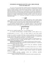
Fig. 1. Five-level cascaded H-Bridge inverter topology. 

a triangle number, it implies the th triangle among 

the 1 triangles in a sector. The triangle leads to 

the simplicity and flexibility of optimizing the switching 

sequences. 

The major feature of the proposed scheme that it can be 

used for any -level 3 inverter without significant 

increase in computations. 

The proposed scheme is explained with the help of a fivelevel 

cascaded H-bridge inverter (also called cascaded inverter) 

topology shown in Fig. 1. The scheme is then extended to a 

-level inverter. The scheme is equally applicable to neutral 

point clamped (NPC) topology [16]. 

The paper is organized in eight sections. Section II introduces 

various modulation modes. Section III introduces the basic idea 

of calculating on-times in the proposed scheme. Section IV explains 

the proposed algorithm for a five-level inverter. Section V 

explains the implementation for a five-level inverter. Section VI 

shows the experimental results for a five-level cascaded inverter. 

Section VII explains the extension of the proposed scheme to a 

-level inverter. Section VIII concludes the paper. 

II. MODULATION INDEX AND MODES OF MODULATION 

In this paper, we define modulation index as 

[4], where is the peak value of fundamental 

voltage generated by the modulator and is the 

peak value of fundamental voltage at six-step operation. For a 

-level cascaded topology 2 1 , 

where is the dc link voltage on each H-bridge as shown 

in Fig. 1. For a NPC topology [16] 2 , 

which is same as two-level inverter [4]. Based on the value 

of the modulation index 0 1 , there are 

three modes of operation [4], namely sinusoidal mode or 

linear mode 0 0.907 , overmodulation mode 

I 0.907 and overmodulation mode II 

1 . The value of 

of overmodulation I and II. 

marks the boundary 

The scheme proposed by Holtz [4] is to modify the magnitude 

and phase of the reference voltage, to achieve the voltage 

control in overmodulation range. In [4], a value of 0.952 is used 

for . Methods such as [5] and [13] also use 

0.952. Tripathi [6] obtains a higher value of as 0.9535 

Fig. 2. Space vector diagram for first sector of a two-level inverter. 

through angular velocity balance of the flux displacement 

vector. In this paper, the value of is taken to be 0.9535 

and a strategy similar to [6] is used. The two-level based 

overmodulation schemes such as [5], [17] can also be easily 

extended to a multilevel inverter using the implementation 

proposed in this paper. 

III. PROPOSED IDEA OF ON-TIME CALCULATION 

FOR A MULTILEVEL INVERTER 

The basic idea of space vector modulation is to compensate 

the required volt-seconds using discrete switching states and 

their on-times. 

In a two-level inverter, on-time calculation [10] is based on 

the location of the reference vector within a sector , 1 

6, where “ ” signifies that can take any integer value from 1 

to 6. 

For the geometry of a sector shown in Fig. 2, the on-times are 

calculated as 

(1) 

(2) 

(3) 

In (2), 2 is the height of a sector , which is 

an equilateral triangle of unity side. In (1)–(3), 1 2 

where is the switching frequency. 

Fig. 3(a) shows the space vector diagram of first sector of 

a five-level inverter. Each sector can be split into 16 triangles 

, where 0 15. In this figure, is the reference

GUPTA AND KHAMBADKONE: GENERAL SPACE VECTOR PWM ALGORITHM 519 

Fig. 3. Space vector diagram—virtual two-level from five-level. 

vector of magnitude at an angle of with axis. We define 

a small vector , which describes the same point in shifted 

system , see Fig. 3(b). It makes angle with the 

axis. 

The volt-seconds required to approximate the small vector 

in the shifted system should be equal to those required 

for actual vector in the original system . Hence, 

we can obtain the on-times for any reference vector by finding 

the on-times of respective small vector . 

First, we identify the triangle where the required reference is 

located and then obtain the coordinates of the small 

vector. The on-time calculations can be performed by using 

the geometry shown in Fig. 3(b), which would result in the 

same on-time equations as those for a classical two-level SVM 

(1)–(3). Since the triangles within any sector of a -level inverter 

are analogous to a sector of a two level inverter, this idea can be 

extended to any level. For example; if is taken as zero vector 

then triangle can be assumed similar to sector 1 of a 

two-level inverter, as per Fig. 2 and Fig. 3(b). Thus, multilevel 

on-time calculation problem is converted to a simple two-level 

on-time calculation problem. This method is described in detail 

in [10] for a three-level inverter. 

In the proposed method, since triangle is considered as the 

basic unit, any suitable vertex can be chosen as virtual zero 

vector. For example, for triangle in Fig. 3(a), any of the three 

vertices , or can be chosen as a virtual zero vector and 

optimal switching sequence [18] can be formed. The order in 

which on-times , , and are used, depends on the order of 

arranging the switching states. 

IV. OPERATION OF FIVE-LEVEL INVERTER IN 

LINEAR AND OVERMODULATION MODE 

The space vector diagram of a three-phase voltage source inverter 

is a hexagon, consisting of six sectors. Here, the operation 

is explained for the first sector, the same is applicable for other 

sectors too. 

Fig. 4. Space vector diagram of the first sector of a five-level inverter showing 

sinusoidal mode, 0 `0.907. 

For a given position of the reference vector, the sector of operation 

1 6 and its angle 0 60 within 

the sector is determined by using (4) and (5), respectively 

(4) 

(5) 

In (4) and (5), 0 360 is the angle of the reference 

vector with respect to axis, is standard math function “integer” 

and is standard math function “remainder.” 

A. Sinusoidal Modulation Mode 0 0.907 

In this mode, the reference vector , moves on a circular 

trajectory as shown in Fig. 4. The tip P of the reference vector 

can be located in any of the 16 triangles; . Per 

Section III, a triangle in Fig. 4 can be treated as a sector of a 

two-level inverter. The objective here is to identify the triangle 

in which the point is located, subsequently using the small 

vector analogy in the virtual two-level geometry, the on-times 

for this triangle can be calculated using two-level on-times 

(1)–(3). 

For simplicity, it can be assumed that the sector 

in Fig. 4 consists of two types of triangles: type 1 and type 2. A 

type 1 triangle has its base side at the bottom, e.g., triangle , 

, 

. A type 2 triangle has its base side at the top, e.g., triangle 

. 

The search for the triangle that has point P can be narrowed 

down by using two integers and , which are dependent on 

the coordinate of point P as 

In (6), signifies part of the sector between the lines 

and , e.g., in Fig. 4 

2, it signifies the part of the sector between line segments 

and . In (6), signifies part of the sector between 

the lines and 1 , e.g., in Fig. 4 1, it 

signifies the part of the sector between line segments and 

. These two regions are inclined at 120 . Geometrically, 

the values of and , signify the intersection of these two 

regions. This intersection is either a triangle or rhombus. For 

(6)


the reference vector in Fig. 4(a), 2 and 1, i.e., the 

intersection is rhombus where the tip P of reference 

vector is situated. 

This rhombus is made of two triangles and . Let 

be the coordinates of the point P with respect to the 

point , obtained as 

The slope of is and the slope of diagonal 

is . The triangle where point P is located can be determined 

by comparing the slope of with . Slope comparison 

is done by evaluating the inequality , leading to 

following two results on small vector 

. 

and triangle number 

1) : The point P is within the triangle and 

the small vector is represented by 

. The triangle number is obtained as 

2) : The point P is within the triangle and the 

small vector is represented by 0.5 

. The triangle number is obtained as 

These two results can be generalized to triangles of type 1 and 

type 2 respectively. For example; when the point P is in triangle 

, inequality will be true because triangle is 

a triangle of type 1. The small vector is represented 

by . In (8) and (9), “ ” symbolizes a triangle and 

“ ” the triangle number. Hence, 

th triangle in the sector. 

is an integer and signifies 

Having determined the small vector ( , ) for the reference 

vector, the on-times are now calculated using (1)–(3). 

The triangle in a sector is identified as an integer using a 

simple algebraic expression (8) or (9). It is a byproduct of the 

small vector determination process, so no other computation is 

required. It greatly simplifies the PWM process as switching 

states can be easily mapped with respect to the triangle number 

. The triangle number is formulated to provide a simple 

way of arranging the triangles, leading to ease of identification 

and extension to any level. 

The flowchart in Fig. 7(b) shows the determination of 

on-times and triangle number 

reference vector. 

for the circular trajectory of 

B. Overmodulation Mode I 0.907 0.9535 

This region is marked by nonlinearity. In Fig. 5, the thick 

dotted circle shows the desired trajectory of the reference 

vector . Traditionally, depending on the , the trajectory is 

modified and tip P of the actual vector moves on trajectory 

shown in thick solid lines. i.e. first it moves along 

the circular track , then along the linear track on 

the side of the sector and finally along the 

circular track . This modification in trajectory is intended 

(7) 

(8) 

(9) 


overmodulation mode I, 0.907 ` 0.9535. 

to compensate for the loss in volt-secs. The linear movement 

along is called hexagonal track in this paper. 

We follow an approach similar to [6], to compensate for 

the loss in volt-secs by directly modifying the on-times of the 

switching vectors on circular track rather than modifying the 

reference vector. 

Let be the angle where the reference vector crosses the 

hexagon track, shown by the dotted arrow in Fig. 5. For 

3 the vector moves on hexagonal track and for 

remaining part of the sector on circular track. Using cartesian 

geometry, angle is obtained as 

(10) 

For a given , is a fixed number, so it need not be calculated 

in every switching period. 

1) Hexagonal Portion 3 : For hexagonal 

track, using cartesian geometry, the coordinates of the tip P of 

vector are given in terms of angle and level of inverter , 

as 

(11) 

Knowing the coordinates of from (11), the 

on-times and triangle number can be obtained similar to linear 

mode, as explained below. 

We defined two integers and for (6) to find the triangle 

in which point P lies. Using the same definition of and , 

to find the triangle on which point P lies, these two integers are 

now given as 

(12) 

The tip of the vector resides on one of the four triangles 

, , and . These triangles are of type 1. Using this 

fact, the small vector can be directly obtained from 

, without performing slope comparison. It is given as 

(13)


Knowing , (1) is used to determine the on-time . 

Similar to two-level, on-time is zero for hexagonal track, 

therefore . Triangle number is calculated using 

(8). 

Flowchart in Fig. 7(c) shows the on-times and triangle 

number calculation. Number of computations required for 

hexagonal track in Fig. 7(c) are less than that for circular track 

in Fig. 7(b). 

2) Circular Portion (0 and 3 

3): Here, on-times are obtained using (1)–(3) as described 

before for the linear mode. However, on-times are modified to 

compensate for the loss of volt-secs during the linear trajectory 

as described below. 

In the overmodulation mode I, at a modulation index , the 

loss in volt-seconds over a sector is proportional to 0.907 

[6]. Maximum possible value of is 0.9535. Therefore, maximum 

possible loss in volt-seconds over a sector is proportional 

to (0.9535-0.907). Let us define a compensation factor as the 

ratio of actual loss in volt-secs and maximum loss in volt-secs. 

It is given as 

(14) 

Compensation factor is used for modification of on-times 

for the volt-secs compensation. The varies between 0 and 1, 

for between 0.907 and 0.9535. For a given , is a fixed 

number, and hence need not be calculated in every modulation 

cycle. Further details on can be referred in [6]. 

In Fig. 5, for the circular portion, the point P can be within 

any of the triangles . Type 1 triangles , , , 

and have their two vertices on the side of sector. 

Type 2 triangles , and have their one vertex on 

the side of sector. Let the on-times of the three vertices 

be , , and obtained from (1)–(3) through linear mode of 

modulation. For the two types of triangles, these on-times are 

modified differently as explained below. 

Modifications for Type 1 triangle: Let the on-times of the 

two vertices which are on the side of hexagon be and , 

then the modified on-times are given as 

(15) 

The modifications of on-times in (15) effectively reduce 

the on-times of the inner vector using and increase the 

on-times of the outer vectors. It is explained in [6] that such 

scheme is suitable for fast close loop operation. Similarly, 

the on-times for the type 2 triangle are modified. 

Modifications for Type 2 triangle: Let the on-times of the 

two vertices that are not on the side of hexagon be and 

, then the modified on-times are obtained as 

(16) 


Overmodulation Mode II, 0.9535 `1. 

The modifications of on-times in (16) effectively reduce 

the on-times of the inner vectors and increase the on-times 

of the outer vector using . 

In (15) or (16), there is no compensation at 0.907 as 

0. At 0.9535, the compensation is maximum as 

1 and 0, which corresponds to complete movement along 

the hexagonal track. 

For a given , (14) and (15) or (16) are only modifications 

required to modify the on-times. No other lookup table or solution 

to complicated equations is required. Therefore, complexity 

of implementing overmodulation reduces. It also shows the low 

cost of implementing overmodulation on a microcontroller. 

Above 0.9535, the circular part of the trajectory vanishes and 

the on-time obtained from (15) or (16) is negative which is 

meaningless. Above 0.9535, another mode is used called overmodulation 

II. 

C. Overmodulation Mode II 0.9535 1 

Switching in overmodulation II is characterized by a hold 

angle , shown by the dotted arrow in Fig. 6. For 

3 , the tip P of the vector moves on hexagonal track. 

In Fig. 3, let vectors at vertices and be addressed as 

large vectors. There are a total of six large vectors for the complete 

space vector diagram. For 0 and 3 

3, the vector is held at one of the large vectors. 

Normally, is a nonlinear function of modulation index and 

obtained by a lookup table. In this paper, the hold angle is 

obtained using a strategy similar to [6] where is calculated 

by obtaining the same average normalized angular velocity over 

a sector as the angular velocity of the reference vector. For the 

drives application if is maintained, the angular velocity is 

proportional to modulation index . Hence, at a given , the 

time to traverse an angle is equal to where is a constant. 

Similarly, time: i) to cover the linear portion is equal to 

3 2 0.9535; ii) to hold the vector at the large vectors 

of a sector is 2 1.0; and iii) to cover whole sector is 

3 . A time balance equation can be written as 

(17)


Fig. 7. Flowchart: (a) main routine: overall modulation process, (b) task 1: 

subroutine to calculate the on-times and triangle number for the circular track, 

and (c) task 2: subroutine to calculate the on-times and triangle number for the 

hexagonal track 

Simplification of (17) leads to the following expression for 

holding angle as: 

(18) 

In (18), for a given only two arithmetic operations, i.e., 

one division and one subtraction are required to obtain the hold 

angle . It shows the simplicity of implementing overmodulation 

II. 

Fig. 8. Simplified block diagram of the proposed algorithm. 

For 3 , the on-time calculation is same as 

that during the hexagonal trajectory in overmodulation mode I. 

For 0 and 3 3, the vector is held at 

one of the six large vectors. At 1.0, hexagonal track vanishes 

and vector is only held at the six large vectors sequentially. 

This is six-step operation similar to two-level inverter. 

Therefore, a multilevel inverter when operated at 1.0, 

looses its multilevel characteristics. 

V. IMPLEMENTATION FOR A FIVE-LEVEL INVERTER 

The implementation for a five-level inverter can be understood 

with the help of following block diagram. It has two basic 

units namely a processing unit and a mapping unit. 

A. Processing Unit 

Processing unit is basically a microcontroller. The base 

scheme for processing unit is explained in previous section, and 

summarized in flowchart in Fig. 7. It determines parameters 

such as sector, triangle, and calculates on-times. These details 

are subsequently used by mapping unit to generate gating 

signals. 

B. Mapping Unit 

The job of mapping unit is to generate gating signals for the 

inverter. It uses memory to store sequences of switching states. 

A switching sequence is a set of switching states to be applied 

in a switching period. The structure of a switching sequence depends 

on the trajectory of the vector. There are three possible 

trajectories: i) circular track: for linear modulation mode and 

some part of overmodulation I; ii) hexagonal track: for some 

part in overmodulation I and overmodulation II; and iii) hold 

mode: in overmodulation II. Due to the difference in structures 

of switching sequence among the trajectories, three separate 

memory units M–CR, M–HX, and M–HL are used in mapping 

unit, where CR, HX, and HL stand for circular, hexagonal, and 

hold, respectively. The flowchart in Fig. 7(a) introduces an integer 

parameter , called as track index. It is used for realtime 

implementation. It helps in identifying the memory unit with respect 

to track using three values as: i) 0 for circular track; 

ii) 1 for the hexagonal track; and iii) 2 for the hold 

mode. The is independent of the level of inverter. 

There exist 125 5 switching states for fivelevel 

inverter, where , , 2 1 0 1 2 . In Fig. 3, we 

show the switching states for first sector in the space vector diagram. 

A phase-leg state describe the “ON” 

or “OFF” conditions of the switches in the respective phase. In 

Fig. 1, , , and ,


Fig. 9. Switching state at a memory location—ON/OFF signals for the power 

switches. 

where . Hence, essentially four signals are required 

to control the eight switches of a phase-leg. Equivalently, 

each requires 4 b to store the state of the respective 

phase-leg. To this end, 12 b of memory in Fig. 9 stores 

a switching state at a memory location in M–CR, M–HX, and 

M–HX units. Due to the difference in the switching sequences 

in these units, the order in which switching states are organized 

in memory units differ from one another. 

1) Memory Unit for Circular Track (M–CR): On circular 

track tip P of the reference vector is positioned within a triangle 

. There are redundant switching states at the vertices 

of the triangles. Due to redundant states, there could be 

several switching sequences for a triangle. For example, for the 

range 0.5236 0.7854, at a switching period, the tip of 

the reference vector can be situated in triangle . For this triangle, 

following four sequences can be formed with minimum 

switching losses. 

Sequence 1: 

. 

Sequence 2: 

. 

Sequence 3: 

. 

Sequence 4: 

. 

The subscript on a switching state is stage of the sequence. 

Stages 0 3 and 3 0 are the set and reset part of the sequence. 

Similarity to a two-level SVPWM can be seen here. Subscript 

“0” and “3” represent the same vertex, and correspond to virtual 

zero vector of the two-level space vector diagram. 

Generally, a continuous PWM sequence have four stages as 

shown above, and a discontinuous PWM sequences have three 

stages [19]. The counter in processing unit generates stage 

number using the on-times , and . Here, 0 3 

for continuous SVM and 0 2 for discontinuous SVM. 

Among the various switching sequences for a triangle, only 

one can be applied at a switching period. Following examples 

explain the selection of a switching sequence using triangle . 

Example 1: Common Mode Voltage Reduction—In [20], 

a common mode voltage reduction scheme is given. The 

five-level ( -level) space vector diagram is converted to 

equivalent three-level ( -1-level) space vector diagram by 

retaining the switching states which generate zero common 

mode voltage. Due to the absence of redundancies, only 

one switching sequence exists for every triangle. 

Example 2: Intertriangle Switching Losses Minimization—There 

are two possible transitions of the reference 

vector for triangle . The transition depends on : 

Fig. 10. Memory address for circular track. 

i) for the range 0.5236 0.6614, the transition is 

, and Sequence 1 (or 2) is selected and ii) for the 

range 0.6614 0.7854, the transition is , 

and Sequence 3 (or 4) is selected. Here, “ ” signifies 

transition between triangles. 

Example 3: DC-link Balancing in NPC topology—DClink 

balancing is a key issue [21], [22] for NPC topology. 

To have a better control authority over dc-link balance, a 

sequence is selected whose virtual zero vector has highest 

duty ratio among the three duty ratios, i.e., , , and 

for triangle . Therefore, in triangle , Sequence 

1 (or 2) is selected if is maximum, Sequence 3 is selected 

if is maximum and Sequence 4 is selected if 

is maximum. This technique is well known for three-level 

inverter. 

These examples show that the selection of a switching sequence 

is dependent on the modulation scheme. For a given 

scheme, a set of relevant switching sequences can be identified 

for every triangle and stored in memory unit in contiguous locations. 

This is an off-line process. 

To this end, an 11-b address is given in Fig. 10. This address 

identifies a memory location in M-CR unit. It is divided into 

four parts: i) “Sector”: 3b , as for sector number 

, 1 6; ii) “Triangle”: 4b , as for triangle 

number , 15; iii) “Sequence”:2b , considering 

a retention of maximum four sequences per triangle; 

and iv) “Stage”: 2b , considering three or four 

stages per sequence with respect to continuous or discontinuous 

SVM, respectively. 

For a given modulation scheme, at any switching period, the 

processing unit calculates these parameters. Using these parameters, 

a memory location (switching state) is identified. Since 

the contents of a memory location represent “ON” or “OFF” 

condition for the switches of the inverter, they can be directly 

applied for generating gating signals. The proposed mapping 

concept can be used to implement a variety of schemes as explained 

above. It shows the generality of the proposed mapping 

concept. 

2) Memory Unit for Hexagonal Track (M–HX): On hexagonal 

track in Figs. 5 and 6, the tip P of the vector moves along 

on a side of one of the triangles , , , and 

. There is one switching state at a vertex on hexagonal 

track. The switching states at the nearest two vectors are utilized 

to form a switching sequence. For example; for triangle , 

the switching sequence is 

. Conclusively, a switching sequence 

on hexagonal track has only two stages. The counter in 

processing unit generates stage number using on-times 

and . 

To this end, an 8-b address is given in Fig. 11. This address 

identifies a memory location in M–HX unit. It is divided into 

three parts: i) “Sector”: 3b ; ii) “Triangle”: 4b 

; and iii) “Stage”: 1b , as only two stages


Fig. 11. Memory address for hexagonal track. 

Fig. 12. Memory address for hold mode. 

Fig. 13. Voltage † , current s , and FFT of voltage † at a0.90. 

exist. Due to the absence of redundant switching states, only 

one switching sequence exists for a triangle on hexagonal track. 

3) Memory Unit for Hold Mode (M-HL): In hold mode, the 

vector is held at a large vector. The switching state at this 

vertex, e.g., (2, 2, 2) is applied for full switching period. Unlike 

other two tracks, the switching sequence contains only one 

stage in hold mode. To this end, a 3-b address is given in Fig. 11, 

to identify a memory location in M–HL unit. The “Triangle,” 

“Sequence,” and “Stage” are not required here. 

This implementation is advantageous as compared to implementation 

of carrier based schemes for a multilevel inverter. In 

carrier based schemes, a separate controller might be required 

for every H-bridge [20] as every phase-leg is controlled separately. 

In such implementation, the synchronization of the controllers 

might lead to implementation complexity. On the other 

hand, using the proposed scheme a single controller unit generates 

the gating signals for all the switches of the inverter. 

The proposed scheme is applicable to both NPC and cascaded 

inverter. For a given level, the two topologies have same space 

vector diagram and equal number of power switches, so the cost 

of peripherals does not change. The processing unit is same for 

both the topologies. For a given level, there are equal number of 

controllable switches in these topologies but their arrangement 

is different. Hence, for a given switching state, the gating signals 

or the set of bits at a memory location in Fig. 9 differ for the 



two topologies. Hence, the mapping unit should be redesigned 

while changing from one topology to the other. We show the 

implementation of the proposed scheme for a three-level NPC 

inverter in [23]. 

VI. EXPERIMENTAL RESULTS FOR FIVE-LEVEL 

CASCADED INVERTER 

The algorithm is implemented using a dSPACE DS1104 card, 

due to its availability. Owing to the simplicity of the algorithm


Fig. 16. Line voltage for seven-level inverter at (a) a 0.89, (b) a 0.93, and (c) a 0.97. 

it can be easily implemented on a fixed point DSP as well. The 

algorithm is tested on a laboratory prototype of a five-level cascaded 

inverter. The test was performed on a 0.75-kW induction 

motor at 100 V, fundamental frequency 50 Hz 

and sampling frequency 5 kHz. Here, is voltage 

applied on each H-bridge module per Fig. 1. 

Figs. 13–15(a) show the line voltage and current at 

a modulation index of 0.90, 0.94, and 0.98 corresponding to 

linear mode, overmodulation mode I and overmodulation mode 

II, respectively. 

Figs. 13–15(b) show the linear RMS FFT of line voltage 

at a modulation index of 0.90, 0.94, and 0.98 corresponding to 

the linear mode, overmodulation mode I and overmodulation 

mode II, respectively. In Figs. 13–15(b), the top right quarter 

is complete FFT. This FFT is 10 vertically magnified to study 

various harmonics which occupies the remaining three quarters. 

Weighted total harmonic distortion WTHD [19] is given to study 

the harmonic losses. The is RMS value of fundamental 

component of the line voltage. For a cascaded inverter, theoretical 

RMS value of is given as . 

The error between experimental and theoretical value is less 

than 1% for the three cases. The error between simulation and 

theoretical value is less than 0.4% for at any . 

VII. EXTENSION OF THE PROPOSED SCHEME 

TO A -LEVEL INVERTER 

The block diagram in Fig. 8 describes the proposed scheme 

and its implementation for a five-level inverter. Some changes 

can be expected when it is applied to a -level inverter. We 

discuss below, the processing unit with respect to computational 

load, and mapping unit with respect to memory requirement. 

A. Processing Unit 

The processing unit calculates on-times and basic parameters 

to apply a switching state. The base scheme in Fig. 8 is essentially 

the flowchart in Fig. 7. This flowchart is given for a -level 

inverter. The main routine in Fig. 7(a) and sub-routine 

in Fig. 7(c) use as a linear constant, showing that number of 

computations are same for any value of . Whereas in 

Fig. 7(b) is independent of . Therefore, the number of computations 

for the base scheme in processing unit remain same for 

any value of . Conclusively, the same processing unit can be 

used for any level without any change. 

B. Mapping Unit 

Conceptually, the mapping unit for -level is the same as 

shown in Fig. 8. However, there are the following two structural 

changes in the number of bits at a memory location in Fig. 9 and 

its address in Figs. 10 and 11. 

1) In Fig. 9, for -level, bits are required to store a 

switching state at a memory location. 

2) The bits required for “Triangle” in Figs. 10 and 11 change, 

as there are 1 triangles per sector. For example, 7 b 

are required for “Triangle” part for an 11-level inverter as 

there are 100 triangles per sector. Except for “Triangle,” 

other parts in Figs. 10 and 11 remain unaffected by the 

change in . 

Commercially available EPROM chips of 1-, 4-, 16-, 32-, and 

64-kB sizes fulfill the memory requirement of mapping unit, 

to implement the proposed scheme for three-level, five-level, 

seven-level, nine-level, and 11-level inverter, respectively. This 

estimation is based on the memory structure shown in Figs. 9–12 

where the bits at memory location are directly used for generating 

gating signals. This estimation may change with the modulation 

scheme. The memory requirement increases with ,as 

switching states . The size of the memory is reduced to half 

if a two-step cascaded memory is used. 

Fig. 16(a)–(c) show the line voltage for a seven-level 

cascaded inverter at a modulation index of 0.89, 0.93, and 0.97. 

For this implementation, the same processing unit is used as 

for five-level without any change. The mapping unit is modified 

per the requirements of a seven-level inverter. The test was performed 

at 100 V, fundamental frequency 50 Hz, 

and sampling frequency 5 kHz. 

VIII. CONCLUSION 

This paper proposes a SVPWM based scheme to perform 

overmodulation for a multilevel inverter, and its implementation. 

The position of the vector is identified using an integer parameter, 

called a triangle number. The switching sequences are 

mapped with respect to the triangle number. The on-times calculation 

is based on on-time calculation for two-level SVPWM. 

The on-time calculation equations do not change with the triangle. 

A simple method of calculating on-times in the overmodulation 

range is used, hence, a solution to complex equations 

and lookup tables are not required. This leads to ease of implementation. 

There are no significant changes in computation with 

the increase in level. The proposed implementation is general in 

nature and can be applied to a variety of modulation schemes. 

The implementation is shown for a five-level and seven-level


cascaded inverter. The experimental results are provided. The 

proposed method can be easily implemented using a commercially 

available motion control DSP or micro-controller, which 

normally supports only two-level modulation. 

REFERENCES 

[1] J. Rodriguez, J.-S. Lai, and F. Z. Peng, “Multilevel inverters: a survey 

of topologies, controls, and applications,” IEEE Trans. Ind. Electron., 

vol. 49, no. 4, pp. 724–738, Aug. 2002. 

[2] P. Hammond, “A new approach to enhance power quality for medium 

voltage ac drives,” IEEE Trans. Ind. Appl., vol. 33, no. 1, pp. 202–208, 

Jan./Feb. 1997. 

[3] L. M. Tolbert, F. Z. Peng, and T. G. Habetler, “Multilevel converters 

for large electric drives,” IEEE Trans. Ind. Appl., vol. 35, no. 1, pp. 

36–44, Jan./Feb. 1999. 

[4] J. Holtz, W. Lotzkat, and A. M. Khambadkone, “On continuous control 

of pwm inverters in overmodulation range including six-step,” IEEE 

Trans. Power Electron., vol. 8, no. 4, pp. 546–553, Oct. 1993. 

[5] D.-C. Lee and G.-M. Lee, “A novel overmodulation technique for 

space-vector pwm inverters,” IEEE Trans. Power Electron., vol. 13, 

no. 6, pp. 1144–1151, Nov. 1998. 

[6] A. Tripathi, A. M. Khambadkone, and S. K. Panda, “Direct method of 

overmodulation with integrated closed loop stator flux vector control,” 

IEEE Trans. Power Electron., vol. 20, no. 5, pp. 1161–1168, Sep. 2005. 

[7] A. M. Massoud, S. J. Finney, and B. W. Williams, “Control techniques 

for multilevel voltage source inverters,” in Proc. Power Electron. Spec., 

Jun. 2003, vol. 1, pp. 171–176. 

[8] N. Celanovic and D. Boroyevich, “A fast space vector modulation algorithm 

for multilevel three phase converters,” IEEE Trans. Ind. Appl., 

vol. 37, no. 2, pp. 637–641, Mar./Apr. 2001. 

[9] R. S. Kanchan, M. R. Baiju, K. K. Mohapatra, P. P. Ouseph, and K. 

Gopakumar, “Space vector pwm signal generation for multilevel inverters 

using only the sampled amplitudes of reference phase voltages,” 

Proc. Inst. Elect. Eng., vol. 152, no. 2, pp. 297–309, Mar. 2005. 

[10] A. K. Gupta, A. M. Khambadkone, and K. M. Tan, “A two-level 

inverter based svpwm algorithm for a multilevel inverter,” in Proc. 

Annu. Conf. IEEE Ind. Electron. Soc. (IECON), Nov. 2004, vol. 2, pp. 

1823–1828. 

[11] J. H. Seo, C. H. Choi, and D. S. Hyun, “A new simplified space-vector 

pwm method for three-level inverters,” IEEE Trans. Power Electron., 

vol. 16, no. 4, pp. 545–550, Jul. 2001. 

[12] B. P. McGrath and D. G. Holmes, “Sinusoidal pwm of multilevel inverters 

in the overmodulation region,” in Proc. IEEE 33rd Annu. Power 

Electron. Spec. Conf. (PESC), Jun. 2002, vol. 2, pp. 485–490. 

[13] S. K. Mondal, B. K. Bose, V. Oleschuk, and J. O. P. Pinto, “Space 

vector pulse width modulation of three-level inverter extending operation 

into overmodulation region,” IEEE Trans. Power Electron., vol. 

18, no. 2, pp. 604–611, Mar. 2003. 

[14] M. Saeedifard, A. R. Bakhshai, G. Joos, and P. Jain, “Extending the 

operating range of the neuro-computing vector classification space 

vector modulation algorithm of three-level inverters into overmodulation 

region,” in Proc. IEEE 38th Ind. Appl. Conf., Oct. 2003, vol. 1, 

pp. 672–677. 

[15] S. K. Mondal, J. O. P. Pinto, and B. K. Bose, “A neural-network-based 

space-vector pwm controller for a three-level voltage-fed inverter induction 

motor drive,” IEEE Trans. Power Electron., vol. 38, no. 3, pp. 

660–669, May/Jun. 2002. 

[16] A. Nabae, I. Takahashi, and H. Akagi, “A new neutral-point clamped 

pwm inverter,” IEEE Trans. Ind. Appl., vol. IA-17, no. 5, pp. 518–523, 

Sep./Oct. 1981. 

[17] S. Bolognani and M. Zigliotto, “Novel digital continuous control of 

svm inverters in the overmodulation range,” IEEE Trans. Ind. Appl., 

vol. 33, no. 2, pp. 525–530, Mar./Apr. 1997. 

[18] B. P. McGrath, D. G. Holmes, and T. A. Lipo, “Optimized space vector 

switching sequences for multilevel inverters,” IEEE Trans. Power Electron., 

vol. 18, no. 6, pp. 1293–1301, Nov. 2003. 

[19] D. G. Holmes and T. A. Lipo, Pulse Width Modulation for Power Converters. 

New York: Wiley, 2003. 

[20] P. C. Loh, D. G. Holmes, Y. Fukuta, and T. A. Lipo, “Reduced 

common-mode modulation strategies for cascaded multilevel inverters,” 

IEEE Trans. Ind. Appl., vol. 39, no. 5, pp. 1386–1395, 

Sep./Oct. 2003. 

[21] T. Ishida, K. Matsuse, K. Sugita, L. Huang, and K. Sasagawa, “Dc 

voltage control strategy for a five-level converter,” IEEE Trans. Power 

Electron., vol. 15, no. 3, pp. 508–515, May 2000. 

[22] N. Celanovic and D. Boroyevich, “A comprehensive study of neutral 

point voltage balancing problem in three level neutral point clamped 

voltage source pwm inverters,” IEEE Trans. Power Electron., vol. 15, 

no. 2, pp. 242–249, Mar. 2000. 

[23] A. K. Gupta and A. M. Khambadkone, “A general space vector pwm 

algorithm for a multilevel inverter including operation in overmodulation 

range, with a detailed modulation analysis for a three-level npc 

inverter,” in Proc. PESC, Jun. 2005, pp. 2527–2533. 

Amit Kumar Gupta (S’04) was born in India, 

in 1978. He received the B.E. degree in electrical 

engineering from the Indian Institute of Technology, 

Roorkee, in 2000 and is currently pursuing the Ph.D. 

degree at the National University of Singapore, 

Singapore. 

From 2000 to 2003, he worked for Bechtel India 

Pvt., Ltd., New Delhi and Samsung Heavy Industries, 

Ltd., Korea. His research interests include PWM for 

multilevel converters, power electronics, and motion 

control. 

Ashwin M. Khambadkone (SM’04) received 

the Dr.-Ing. degree from Wuppertal University, 

Wuppertal, Germany, in 1995 and the Graduate 

Certificate in education from the University of 

Queensland, Brisbane, Australia. 

At Wuppertal, he was involved in research and industrial 

projects in the areas of PWM methods, fieldoriented 

control, parameter identification, and sensorless 

vector control. From 1995 to 1997, he was a 

Lecturer at the University of Queensland. He was also 

at the Indian Institute of Science, Bangalore, India in 

1998. Since 1998, he has been an Assistant Professor at the National University 

of Singapore. His research activities are in the control of ac drives, design and 

control of power electronic converters, and fuel cell based systems. 

Dr. Khambadkone received the Outstanding Paper Award in 1991 and the 

Best Paper Award in 2002 both which appeared in the IEEE TRANSACTIONS ON 

INDUSTRIAL ELECTRONICS.

A General Space Vector PWM Algorithm for Multilevel Inverters ...

Create successful ePaper yourself

Delete template?

Save as template?