CHAPTER 2
CHAPTER 2
CHAPTER 2

Create successful ePaper yourself
Turn your PDF publications into a flip-book with our unique Google optimized e-Paper software.
<strong>CHAPTER</strong> 2<br />
SINGLE PHASE PULSE WIDTH MODULATED INVERTERS<br />
2.1 Introduction<br />
The dc-ac converter, also known as the inverter, converts dc power to ac power<br />
at desired output voltage and frequency. The dc power input to the inverter is<br />
obtained from an existing power supply network or from a rotating alternator through<br />
a rectifier or a battery, fuel cell, photovoltaic array or magneto hydrodynamic<br />
generator. The filter capacitor across the input terminals of the inverter provides a<br />
constant dc link voltage. The inverter therefore is an adjustable-frequency voltage<br />
source. The configuration of ac to dc converter and dc to ac inverter is called a dc-<br />
link converter.<br />
Inverters can be broadly classified into two types, voltage source and current<br />
source inverters. A voltage–fed inverter (VFI) or more generally a voltage–source<br />
inverter (VSI) is one in which the dc source has small or negligible impedance. The<br />
voltage at the input terminals is constant. A current–source inverter (CSI) is fed with<br />
adjustable current from the dc source of high impedance that is from a constant dc<br />
source.<br />
A voltage source inverter employing thyristors as switches, some type of forced<br />
commutation is required, while the VSIs made up of using GTOs, power transistors,<br />
power MOSFETs or IGBTs, self commutation with base or gate drive signals for their<br />
controlled turn-on and turn-off.<br />
16
A standard single-phase voltage or current source inverter can be in the half-<br />
bridge or full-bridge configuration. The single-phase units can be joined to have<br />
three-phase or multiphase topologies. Some industrial applications of inverters are for<br />
adjustable-speed ac drives, induction heating, standby aircraft power supplies, UPS<br />
(uninterruptible power supplies) for computers, HVDC transmission lines, etc.<br />
In this chapter single-phase inverters and their operating principles are<br />
analyzed in detail. The concept of Pulse Width Modulation (PWM) for inverters is<br />
described with analyses extended to different kinds of PWM strategies. Finally the<br />
simulation results for a single-phase inverter using the PWM strategies described are<br />
presented.<br />
2.2 Voltage Control in Single - Phase Inverters<br />
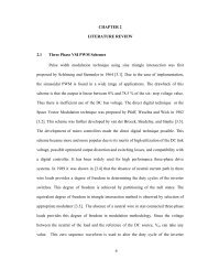
The schematic of inverter system is as shown in Figure 2.1, in which the<br />
battery or rectifier provides the dc supply to the inverter. The inverter is used to<br />
control the fundamental voltage magnitude and the frequency of the ac output<br />
voltage. AC loads may require constant or adjustable voltage at their input terminals,<br />
when such loads are fed by inverters, it is essential that the output voltage of the<br />
inverters is so controlled as to fulfill the requirement of the loads. For example if the<br />
inverter supplies power to a magnetic circuit, such as a induction motor, the voltage<br />
to frequency ratio at the inverter output terminals must be kept constant. This avoids<br />
saturation in the magnetic circuit of the device fed by the inverter.<br />
17
Battery<br />
or<br />
Rectifier<br />
Vd<br />
Cd<br />
Figure 2.1: Schematic for Inverter System<br />
Inverter<br />
AC<br />
Voltage<br />
The various methods for the control of output voltage of inverters can be classified as:<br />
(a) External control of ac output voltage<br />
(b) External control of dc input voltage<br />
(c ) Internal control of the inverter.<br />
The first two methods require the use of peripheral components whereas the third<br />
method requires no external components. Mostly the internal control of the inverters<br />
is dealt, and so the third method of control is discussed in great detail in the following<br />
section.<br />
2.2.1 Pulse Width Modulation Control<br />
The fundamental magnitude of the output voltage from an inverter can be<br />
controlled to be constant by exercising control within the inverter itself that is no<br />
external control circuitry is required. The most efficient method of doing this is by<br />
Pulse Width Modulation (PWM) control used within the inverter. In this scheme the<br />
inverter is fed by a fixed input voltage and a controlled ac voltage is obtained by<br />
18
adjusting the on and the off periods of the inverter components. The advantages of the<br />
PWM control scheme are [10]:<br />
a) The output voltage control can be obtained without addition of any external<br />
components.<br />
b) PWM minimizes the lower order harmonics, while the higher order<br />
harmonics can be eliminated using a filter.<br />
The disadvantage possessed by this scheme is that the switching devices used in the<br />
inverter are expensive as they must possess low turn on and turn off times,<br />
nevertheless PWM operated are very popular in all industrial equipments. PWM<br />
techniques are characterized by constant amplitude pulses with different duty cycles<br />
for each period. The width of these pulses are modulated to obtain inverter output<br />
voltage control and to reduce its harmonic content. There are different PWM<br />
techniques which essentially differ in the harmonic content of their respective output<br />
voltages, thus the choice of a particular PWM technique depends on the permissible<br />
harmonic content in the inverter output voltage.<br />
2.2.2 Sinusoidal-Pulse Width Modulation (SPWM)<br />
The sinusoidal PWM (SPWM) method also known as the triangulation, sub<br />
harmonic, or suboscillation method, is very popular in industrial applications and is<br />
extensively reviewed in the literature [1-2]. The SPWM is explained with reference to<br />
Figure 2.2, which is the half-bridge circuit topology for a single-phase inverter.<br />
19
Vd<br />
Vd<br />
2<br />
Vd<br />
2<br />
+<br />
C<br />
+<br />
C<br />
S 11<br />
Figure 2.2: Schematic diagram for Half-Bridge PWM inverter.<br />
S 12<br />
For realizing SPWM, a high-frequency triangular carrier wave v is<br />
compared with a sinusoidal reference v of the desired frequency. The intersection of<br />
vc r<br />
and waves determines the switching instants and commutation of the modulated<br />
v<br />
pulse. The PWM scheme is illustrated in Figure 2.3 a, in which v is the peak value of<br />
triangular carrier wave and v that of the reference, or modulating signal. The figure<br />
shows the triangle and modulation signal with some arbitrary frequency and<br />
magnitude. In the inverter of Figure 2.2 the switches S and S are controlled based<br />
on the comparison of control signal and the triangular wave which are mixed in a<br />
comparator. When sinusoidal wave has magnitude higher than the triangular wave the<br />
comparator output is high, otherwise it is low.<br />
r c v 11<br />
v > S is on ,<br />
and<br />
vr vc 12<br />
r<br />
< S is on ,<br />
r<br />
11<br />
12<br />
Vo<br />
Vd<br />
V out =<br />
(2.1)<br />
2<br />
Vd<br />
V out = −<br />
(2.2)<br />
2<br />
20<br />
c<br />
c
Figure 2.3: SPWM illustration (a) Sine-Triangle Comparison (b) Switching Pulses<br />
after comparison.<br />
21<br />
(a)<br />
(b)
The comparator output is processesed in a trigger pulse generator in such a<br />
manner that the output voltage wave of the inverter has a pulse width in agreement<br />
with the comparator output pulse width. The magnitude ratio of<br />
vr is called the<br />
modulation index ( m ) and it controls the harmonic content of the output voltage<br />
i<br />
waveform. The magnitude of fundamental component of output voltage is<br />
proportional to . The amplitude v of the triangular wave is generally kept<br />
mi c<br />
constant. The frequency–modulation ratio m is defined as<br />
f<br />
f<br />
t<br />
m f = (2.3)<br />
f m<br />
To satisfy the Kirchoff’s Voltage law (KVL) constraint, the switches on the same leg<br />
are not turned on at the same time, which gives the condition<br />
+ S = 1 (2.4)<br />
S11 12<br />
for each leg of the inverter. This enables the output voltage to fluctuate between<br />
Vd and<br />
2<br />
Vd<br />
− as shown in Figure 2.4 for a dc voltage of 200 V.<br />
2<br />
22<br />
v<br />
c
Figure 2.4: Output voltage of the Half-Bridge inverter.<br />
2.3 Single-Phase Inverters<br />
A single-phase inverter in the full bridge topology is as shown in Figure<br />
2.5, which consists of four switching devices, two of them on each leg. The full-<br />
bridge inverter can produce an output power twice that of the half-bridge inverter<br />
with the same input voltage. Three different PWM switching schemes are discussed<br />
in this section, which improve the characteristics of the inverter. The objective is to<br />
add a zero sequence voltage to the modulation signals in such a way to ensure the<br />
clamping of the devices to either the positive or negative dc rail; in the process of<br />
which the voltage gain is improved, leading to an increased load fundamental voltage,<br />
reduction in total current distortion and increased load power factor. In Figure 2.5, the<br />
top devices are assigned to be S11 and S21 while the bottom devices as S12 and S22, the<br />
voltage equations for this converter are as given in the following equations.<br />
23
Vd<br />
Vd<br />
2<br />
o<br />
Vd<br />
2<br />
+<br />
C<br />
+<br />
C<br />
S 11<br />
a<br />
S 12<br />
S 21<br />
S 22<br />
Figure 2.5: Schematic of a Single Phase Full-Bridge Inverter.<br />
V<br />
2<br />
V<br />
2<br />
d ( S11<br />
− S12)<br />
= Van<br />
+ Vno<br />
= Vao<br />
(2.5)<br />
d ( S21<br />
− S22)<br />
= Vbn<br />
+ Vno<br />
= Vbo<br />
(2.6)<br />
V = V −V<br />
(2.7)<br />
ab<br />
an<br />
bn<br />
b<br />
Vab<br />
The voltages and V are the output voltages from phases A and B to an<br />
arbitrary point n, V is the neutral voltage between point n and the mid-point of the<br />
no<br />
DC source. The switching function of the devices can be approximated by the Fourier<br />
series to be equal to<br />
Van bn<br />
1<br />
( 1+<br />
M )<br />
2<br />
where M is the modulation signal which when<br />
compared with the triangular waveform yields the switching pulses [19]. Thus from<br />
Equations 2.4, 2.5, and 2.6, the expressions for the modulation signals are obtained as<br />
M<br />
M<br />
2(<br />
V<br />
+ V<br />
)<br />
an no<br />
11 = (2.8)<br />
Vd<br />
21<br />
2(<br />
Vbn<br />
+ Vno<br />
)<br />
= .<br />
(2.9)<br />
V<br />
d<br />
24<br />
+<br />
-
Equations 2.8 and 2.9 give the general expression for the modulation signals for<br />
single-phase dc-ac converters. The various types of modulation schemes presented in<br />
the literature can be obtained from these equations using appropriate definition for<br />
Van bn no<br />
, V and V . Making use of this concept different modulation schemes have been<br />
proposed some of which are explained in detail in the following sections.<br />
2.3.1 SPWM With Bipolar Switching<br />
In this scheme the diagonally opposite transistors S11, S22 and S21 and S12 are<br />
turned on or turned off at the same time. The output of leg A is equal and opposite to<br />
the output of leg B. The output voltage is determined by comparing the control signal,<br />
and the triangular signal, V as shown in Figure 2.6(a) to get the switching pulses<br />
Vr c<br />
for the devices , and the switching pattern is as follows.<br />
V >V , S11<br />
is on =><br />
r<br />
r<br />
c<br />
V <br />
hence<br />
c<br />
Vbo ao<br />
Vd<br />
ao<br />
2<br />
=<br />
V and S22 is on =><br />
Vd<br />
2<br />
ao − = V and S21 is on =><br />
Vd<br />
bo<br />
2<br />
− = V ; (2.10)<br />
Vd<br />
bo<br />
2<br />
= V ; (2.11)<br />
( t)<br />
= −V<br />
( t)<br />
(2.12)<br />
25
Figure 2.6:Bipolar PWM (a) Sine-triangle comparison (b) Switching pulses for<br />
S11/S22 (c) Switching pulses for S12/S21<br />
Figure 2.7: Bipolar PWM scheme (a) Modulation signal for leg ‘a’ (b) output line-line<br />
voltage (c) load current<br />
26<br />
(a)<br />
(b)<br />
(c)<br />
(a)<br />
(b)<br />
(c)
The line-to-line voltage is given as in Equation 2.13.<br />
V ( ) = V ( t)<br />
−V<br />
( t)<br />
= 2V<br />
( t)<br />
(2.13)<br />
ab t ao bo ao<br />
The peak of the fundamental-frequency component in the output voltage is given as<br />
[10]<br />
V = mV<br />
( m ≤ 1.<br />
0 ) (2.14)<br />
ab<br />
and<br />
V<br />
d<br />
i<br />
d<br />
i<br />
4<br />
< Vab<br />
< Vd<br />
( m i ≥1.<br />
0 ). (2.15)<br />
π<br />
Since the voltage switches between two levels − Vd<br />
and V d , the scheme is called the<br />
Bipolar PWM. The relationship between fundamental input and output voltage in the<br />
overmodulating region is given as [10].<br />
V = MV<br />
(2.16)<br />
o<br />
where<br />
d<br />
2mi −1<br />
2<br />
M = (sin α + α 1−<br />
α ) , m i<br />
π<br />
α = 1/<br />
m .<br />
i<br />
> 1<br />
For a full-bridge inverter with bipolar PWM scheme the output voltage is between<br />
Vd<br />
V d<br />
− and . Figure 2.7 shows the modulation signal, output voltage, and the load<br />
2 2<br />
current for bipolar modulation scheme on a single-phase inverter with an RL load of<br />
10 Ω and 0.125H.<br />
27
For the bipolar PWM switching scheme there is only one modulation signal and the<br />
switches are turned ‘on’ or turned ‘off’ according to the pattern given in Equations<br />
2.10 and 2.11. The input dc voltage was 200 V and the modulation index (mi) was<br />
taken to be 0.8. The switching frequency for the carrier, which is the triangle, is 10<br />
kHz.<br />
2.3.2 SPWM With Unipolar Switching<br />
In this scheme, the devices in one leg are turned on or off based on the<br />
comparison of the modulation signal V with a high frequency triangular wave. The<br />
devices in the other leg are turned on or off by the comparison of the modulation<br />
signal −V<br />
with the same high frequency triangular wave. Figure 2.8 and 2.9 show<br />
the unipolar scheme for a single –phase full bridge inverter, with the modulation<br />
signals for both legs and the associated comparison to yield switching pulses for both<br />
the legs.<br />
r<br />
r<br />
In Figure 2.8 the simulation results show the sine triangle comparison, the<br />
switching pulses for S11 and S21 are shown. The switching for the other two devices is<br />
obtained as S12 = 1 – S11 and S22 = 1- S21. Figure 2.9 shows the phase voltages , line-<br />
to-line voltages obtained from a unipolar PWM scheme , also shown is the load<br />
current. The simulation was carried out for an RL load of R = 10Ω and L = 0.125H.<br />
The dc voltage is 200 V and the switching frequency is 10kHz. The modulation signal<br />
has a magnitude of 0.8, i.e mi = 0.8.<br />
28
Figure 2.8: Unipolar PWM voltage switching scheme (a) Sine triangle comparison<br />
(b) switching pulses for S11 (c) switching pulses for S21.<br />
Figure 2.9: Unipolar PWM voltage switching scheme (a) phase voltage ‘a’ (b) phase<br />
voltage ‘b’ (c) line to line voltage Vab (d) load current<br />
29<br />
(a)<br />
(b)<br />
(c)<br />
(a)<br />
(b)<br />
(c)<br />
(d)
given as<br />
r<br />
The logic behind the switching of the devices in the leg connected to ‘a’ is<br />
V > V : is on and V =<br />
r<br />
c S11 an<br />
V V : is on and V =<br />
r c S11 bn<br />
-V
Table 2.1. Switching state of the unipolar PWM and the corresponding voltage levels.<br />
S 11 S 12 S 21 S 22 V An V Bn Vo = VAn<br />
−VBn<br />
ON - - ON V d 0 V d<br />
- ON ON - 0 V d -V d<br />
ON - ON - V d V d<br />
0<br />
- ON - ON 0 0 0<br />
The fundamental component of the output voltage is given as<br />
V = m V<br />
( m ≤1.<br />
0)<br />
(2.21)<br />
V<br />
o<br />
d<br />
i<br />
d<br />
i<br />
4<br />
< Vo<br />
< Vd<br />
( m i > 1.<br />
0 ). (2.22)<br />
π<br />
2.3.3 SPWM With Modified Bipolar Switching Scheme (MBPWM)[14]<br />
In the inverter employing the bipolar switching scheme, switches are<br />
operated in such a way that during the positive half of the modulation signal one of<br />
the top devices in one of the switching leg is kept on and the two other switching<br />
devices in the other leg are PWM operated, and during the negative half of the<br />
modulation signal one of the bottom switching device is kept on continuously while<br />
the other two switching devices in the other leg are PWM operated. The output<br />
voltage is determined by comparing the control signal Vr<br />
and the triangular wave.<br />
31
The switching pattern along with the sine-triangle comparison is as shown in Figure<br />
2.10. The switching pattern for positive values of modulating signal V is as given<br />
m<br />
V r > V c , S21<br />
is on (2.23)<br />
and V r
Figure 2.11: Modified bipolar PWM scheme (a) line-to-line voltage (b) load current<br />
The switching pattern for negative values of the modulating signal V is given as<br />
m<br />
V r < V c , S21<br />
is on (2.24)<br />
and V r > V c , S22<br />
is on .<br />
The output voltage is given as V ( ) = V ( t)<br />
−V<br />
( t)<br />
, as shown in Figure 2.11. The<br />
o t An Bn<br />
load current is also shown in the same plot. The RL load has an R = 10 Ω and L =<br />
0.125H. The modulation signal for the sine-triangle comparison is 0.8. The switching<br />
pattern for the Modified Bipolar Switching Scheme is as given in Table 2.2.<br />
33<br />
(a)<br />
(b)
Table 2.2. Switching state of the modified bipolar PWM and the corresponding<br />
voltage.<br />
V = V −V<br />
S 11 S 12 S 21 S 22 V An V Bn o An Bn<br />
ON - - ON V d 0 V d<br />
- ON ON - 0 V d -V d<br />
ON - ON - V d V d<br />
0<br />
- ON - ON 0 0 0<br />
From Table 2.2 it can be observed that when the two top or the two bottom devices<br />
are turned on the output voltage is zero.<br />
In the modified bipolar switching scheme the output voltage level changes<br />
between either 0 to -V or from 0 to +V . Since the sign of the modulation signal<br />
d d<br />
decides the switching pattern the analysis of this switching scheme is complex. The<br />
relationship between input and output voltage is given as [14],<br />
V o = mVd<br />
(2.25)<br />
where )<br />
4<br />
m = 0.<br />
5(<br />
mi<br />
+ ( m i < 1.<br />
0 ) . (2.26)<br />
π<br />
Thus from the above equation it can be observed that the fundamental component of<br />
the voltage as obtained from the MBPWM is the maximum when compared to the<br />
other switching schemes even in the linear modulation region; that is when the<br />
modulation index is less than unity.<br />
34
2.3.4 Generalized Carrier-based PWM<br />
given as<br />
In the inverter shown in Figure 2.5, the output voltage and the input current are<br />
V S − S ) = V = V + V<br />
0. 5 d ( 11 12 ao an no<br />
(2.27)<br />
V S − S ) = V = V + V<br />
0. 5 d ( 21 22 bo bn no<br />
(2.28)<br />
I d a ( 11 21<br />
ab<br />
= I S − S )<br />
(2.29)<br />
V = V −V<br />
. (2.30)<br />
an<br />
bn<br />
The voltages V and V are the output voltages from phases ‘a’ and ‘b’ to a arbitrary<br />
an<br />
point while V is the neutral voltage between the point ‘n’ and the mid-point of the<br />
no<br />
DC source. The generalized carrier-based PWM scheme is obtained by defining the<br />
quantity V using the concept of q-d Space Vector representation. A special q-d<br />
no<br />
reference frame transformation to transform the two phase voltages to orthogonal q-d<br />
voltage components is defined as<br />
bn<br />
V q = 0. 5(<br />
Van<br />
+ Vbn)<br />
(2.31)<br />
Vd = 0. 5(<br />
Van<br />
−Vbn)<br />
(2.32)<br />
where and V are the q-axis and the d-axis voltages in an orthogonal coordinate<br />
system. The q-d voltages for each of the possible switching instant are shown in<br />
Table 2.3.<br />
Vq d<br />
35
Table 2.3. Switching state of the generalized carrier based PWM scheme.<br />
S 11 S 21 V ao V bo<br />
V q<br />
V d<br />
- - − 0.<br />
5Vd<br />
− 0.<br />
5Vd<br />
− 0 . 5Vd<br />
−Vno<br />
0<br />
- ON − 0.<br />
5Vd<br />
0 . 5Vd<br />
− Vno<br />
− 0.<br />
5Vd<br />
ON - 0 . 5Vd<br />
− 0.<br />
5Vd<br />
− Vno<br />
0 . 5Vd<br />
ON ON 0 . 5Vd<br />
0 . 5Vd<br />
0 . 5Vd<br />
−Vno<br />
0<br />
Figure 2.12 also shows the space vector representation of the output phase<br />
voltages. To synthesize a given reference output voltage V or equivalently V , the<br />
four vectors shown in the figure are averaged over one switching period for the<br />
inverter<br />
*<br />
qd<br />
V = t V + t V + t V + t V<br />
a<br />
qda<br />
b<br />
qdb<br />
c<br />
qdc<br />
d<br />
qdd<br />
ab<br />
*<br />
qd<br />
(2.33)<br />
where t , t , t , t are the normalized times for which the averaging vector spent in<br />
each of the four quadrants. The normalized times should satisfy the condition that<br />
+ tb<br />
+ tc<br />
+ td<br />
= 1.<br />
The normalized times tc , t can be expressed as some equivalent<br />
time to<br />
such that<br />
a<br />
b<br />
c<br />
d<br />
ta d<br />
t + t = t<br />
(2.34)<br />
c<br />
d<br />
o<br />
or equivalently tc , td<br />
can be written as tc<br />
= γto<br />
which implies td = ( 1−<br />
γ ) to<br />
, γ ∈[<br />
0 1]<br />
so<br />
Equation 2.33 can be written as<br />
*<br />
qd<br />
V = t V + t V + γt V + ( 1−<br />
γ ) t V<br />
(2.35)<br />
a<br />
qda<br />
b<br />
qdb<br />
o<br />
qdc<br />
o<br />
qdd<br />
36
V<br />
[ − Vno , − d ] = fqdd<br />
2<br />
V<br />
[ d − Vno,<br />
0]<br />
= fqda<br />
2<br />
*<br />
fqd<br />
V<br />
[ − Vno − d , 0]<br />
= fqdb<br />
2<br />
V<br />
[ − Vno , d ] = fqdc<br />
2<br />
Figure 2.12: Space vector representation of the voltages in a single-phase inverter.<br />
The time t is the actual time which the vector spends in the null state that is<br />
o<br />
when either both the top or both the bottom devices are off or on at the same time.<br />
This time is split in to two time periods such that<br />
a = tx<br />
and so t b ( 1−<br />
ξ ) tx<br />
t ξ<br />
t a + tb<br />
+ to<br />
= 1;<br />
let t + t = t then<br />
= , where ξ ∈[<br />
0,<br />
1]<br />
and γ ∈[<br />
0,<br />
1]<br />
. The quantities t , t , t are<br />
the normalized times (with respect to the switching period of the converter). Solving<br />
Equation 2.33 we can get the expression for the zero sequence voltage V in terms of<br />
other known quantities as<br />
V<br />
no<br />
*<br />
q<br />
−V<br />
Vd<br />
( 2ξ<br />
−1)<br />
= 0.<br />
5Vd<br />
( 2γ<br />
−1)<br />
−<br />
(2.34)<br />
V ( 2ξ<br />
−1)<br />
− 2V<br />
d<br />
*<br />
d<br />
Equations 2.8, 2.9, along with 2.34 constitute the generalized discontinuous PWM<br />
scheme for the single-phase inverter. An infinite number of possibilities for the<br />
discontinuous PWM exist depending on the choice of ξ and γ .<br />
37<br />
a<br />
no<br />
b<br />
a<br />
b<br />
x<br />
o
2.4 Bipolar and Modified Bipolar PWM Schemes with Zero Sequence Voltage<br />
In the PWM modulation scheme with bipolar voltage switching, the<br />
diagonally opposite switching devices are switched as switch pairs resulting in an<br />
output voltage switching between -V and V . The zero sequence voltage expression<br />
for the bipolar schemes is given as,<br />
d d<br />
V = 0 . 5V<br />
( 2γ<br />
−1)<br />
as the q-axis voltage is zero<br />
no<br />
(refer Equations 2.31 and 2.32). If γ is so chosen so as to locate the zero sequence<br />
voltage to be centered about the peak of the modulation signal, we can achieve higher<br />
fundamental component of the load voltage and less switching because the effect of<br />
the zero sequence is to increase the modulation signal to more than unity. In which<br />
case the comparison of the triangle and the modulation signal would yield continuous<br />
‘on’ or ‘off’ of the switching device for a long period of time as when compared to<br />
the regular sine triangle comparison.<br />
2.5 Implementation of the Bipolar and the Modified bipolar PWM Schemes for<br />
an RL load<br />
d<br />
The single-phase inverter in the full-bridge topology has been simulated in<br />
Matlab/Simulink for a RL load with R = 10Ω and L = 0.05 H. The modulation signals<br />
(for a modulation index of 0.8) for the switching devices have been obtained from the<br />
TMSLF2407, Texas Instruments DSP. Figure 2.13 shows the simulation result of<br />
bipolar PWM with the zero-sequence voltage while without the zero sequence was<br />
already shown in Figures 2.8 and 2.9. The simulation results for the modified bipolar<br />
PWM scheme with the zero-sequence voltage are as shown in Figures 2.14. In the<br />
38
simulation the dc voltage was assumed to be 200 V and the modulation index to be<br />
0.8.<br />
Figure 2.13: Bipolar PWM scheme (a) modulation signal (b) &(c) switching pulses<br />
S11/S22 and S21/S12 respectively.<br />
39<br />
(a)<br />
(b)<br />
(c)<br />
(d)<br />
(e)
Figure 2.14: Modified bipolar PWM scheme (a) modulation signal (b), (c), (d) & (e)<br />
switching pulses S11, S12, S21 and S22 (f) line-to-line voltage (g) load current.<br />
40<br />
(a)<br />
(b)<br />
(c)<br />
(d)<br />
(e)<br />
(f)<br />
(g)
2.6 Experimental Results<br />
The experimental results for the above schemes tested in<br />
simulation are presented in Figures 2.15, 2.16, 2.17, and 2.18 for both bipolar and the<br />
modified bipolar PWM strategy with and without the zero-sequence voltage. The RL<br />
–load has an R = 10Ω and L = 0.05H. Table 2.4 shows the comparison between the<br />
four modulation schemes.<br />
Table2.4: Comparative experimental results for the various modulation schemes<br />
Modulation Scheme VRMS IRMS Vf If VTHD ITHD IPEAK PF<br />
Bipolar 49.6 1.6965 48 1.694 25 1.87 2.479 0.407<br />
Bipolar with Vno 56.34 1.948 55 1.949 21.8 1.25 2.769 0.407<br />
ModifiedBipolar 62.5 2.158 59.97 2.148 30.79 10.507 3.228 0.397<br />
ModifiedBipolar with Vno 65.59 2.284 63.39 2.281 26.51 8.763 3.395 0.402<br />
41
Figure 2.15: Bipolar switching scheme, starting from top (1) the load voltage (2) the<br />
load current (3) modulation signal with mi = 0.8.<br />
Figure 2.16: Bipolar switching scheme with zero sequence voltage, (1) load<br />
voltage (2) the load current (3) modulation signal.<br />
42
Figure 2.17: Modified bipolar switching scheme,(1) load voltage (2) load<br />
current (3) modulation signal for one leg (4) modulation signal for the other leg with<br />
mi= 0.8<br />
Figure 2.18: Modified bipolar switching scheme with zero sequence voltage (1)<br />
load voltage (2) load current (3) modulation signal for one leg (4) modulation signal<br />
for the other leg with mi = 0.8 and zero sequence added.<br />
43
Thus the discontinuous PWM modulation for the same reference output<br />
voltage gives higher rms voltages and currents, improved power factor, better voltage,<br />
and current total harmonic distortion factor, that is a low value for current and voltage<br />
THD.<br />
It would appear that the modified bipolar discontinuous PWM scheme is the<br />
best modulation method with the highest output voltage among all while the bipolar<br />
discontinuous PWM scheme gives the best performance in terms of current purity. It<br />
is concluded that the discontinuous PWM modulation methodology results in<br />
improved output voltage magnitude and high waveform fidelity in some cases while<br />
in others the current purity is enhanced when compared to the classical modulation<br />
schemes.<br />
One important realization by using the modulation schemes with the zero-<br />
sequence voltages added is that the switching losses are reduced. The switching<br />
devices are PWM operated in which at every switching period instant the devices are<br />
turned ‘on’or ‘off’. The advantage of using PWM method for operating the switching<br />
devices is to reduce the output harmonics, but the cost to buy this advantage is paid<br />
off for the switching losses, but with the zero-sequence added the switching per<br />
device is reduced and hence the switching losses are reduced.<br />
44