the best probability model for the exacta

ASAC 2005 Conference L.M. Gibson (student)
Toronto, Ontario E.S. Rosenbloom
I.H. Asper School of Business
University of Manitoba
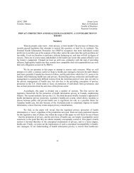
THE BEST PROBABILITY MODEL FOR THE EXACTA
The most heavily wagered bet at the racetrack is the exacta, which looks at the top two
horses to cross the finish line in the exact order. The success of this bet depends on
the probability that the two horses chosen to win and place are correct. It is
commonly assumed in literature that data from the win pool, in association with such
models as Harville (1973) or Henery (1981) provide more accurate subjective
probabilities of the exacta outcome than the data from the exacta pool. Ziemba and
Hausch (1985) and Asch and Quandt (1987) use this assumption to find wagers with
theoretical positive expectation in the exacta pool. In this paper, an SPRT-like test is
used to test this supposition. Results establish that this assumption is false: data from
the exacta pool provides the most accurate estimate of exacta probabilities.
Introduction
All bets at North American racetracks are placed under a pari-mutuel system, developed in the
late 19 th century by Pierre Oller, whereby winners divide the total amount bet, after deducting
track operating expenses, racing purses and taxes, in proportion to individual wagers. Under
this system, players bet against each other, not the racetrack and consequently ‘beat the races’
only when they ‘beat the crowd.’
The exacta wager has replaced the win bet in terms of popularity in recent years, accounting for
approximately 30% of total bets placed at the racetrack (www.churchhilldowns.com). One
suggestion for its popularity is the notion of ‘smart money’: those who have inside information
will avoid straight wagers where odds are continuously displayed on the tote board and instead
place their wagers in the exacta pool where odds are displayed less frequently. In order to
capitalize on these apparent inefficiencies however, an accurate estimate of the win and place
combination yielding the highest probability will help to facilitate positive returns. The
objective thus becomes to determine the method that calculates the most accurate probabilities
for win and place combinations.
Past literature including Ziemba and Hausch (1985) and Asch and Quandt (1987) state that win
pool probabilities are reasonably accurate estimates for win bets and therefore the parallel can
be drawn that win probabilities, alongside models such as Harville (1973) or Henery (1981), can
be applied to the exacta pool (in addition to place, show, quinella and triactor) to capitalize on
inefficiencies.
Before accepting this viewpoint however, it is valuable to question the assumption that win
probabilities can be used to estimate win bets reasonably well. This assumption is largely based
on the observation that horses that have fraction ‘p’ of the win pool, win approximately fraction
‘p’ of the races. To support this assumption would be equivalent to assuming that because it
32

snows 36 days a year in Winnipeg, the probability of snow on any given day is 10% even on a
day in July. This debate aside however, the overall notion that win probabilities are more
accurate than the probabilities generated from the exacta pool is also questionable. This
supposition is explored, and in doing so is the first to empirically test the Harville and Henery
models against the probabilities produced from the exacta pool. Specifically, this paper
compares three methods from which exacta probabilities can be calculated, namely Harville;
Henery; and the exacta pool to determine which model is statistically best.
The Harville Model
The Harville model is the simplest and probably the most commonly used model by academics
and bettors alike. This method calculates the probability for exacta combinations in terms of
win probabilities only. This model assumes that if horse ‘i’ wins the race, the conditional
probability of horse ‘j’ coming in second is given by
Pj|i = Pj / 1-Pi (1)
where Pi and Pj are the probabilities of horse ‘i’ and ‘j’ winning the race. The probability of a
horse winning the race is estimated by using the fraction of the win pool bet on that horse.
Combining this with the win probability for the first place horse, the probability of an i-j exacta
becomes
Pij = PiPj /(1-Pi) (2)
To illustrate the above formula, consider the following data from the 9 th race at Belmont Park on
Sunday September 26 th , 2004:
Wager Winning
Type Number Paid Pool Win Take
Exacta 2-3 $26.00 $270,499.00 14.00%
From the above data, Pij can be calculated:
Horse No. Odds Breakage Pj
2 0.30 0.025 0.649
3 30.75 0.125 0.027
P23 = (.649)(.027) / (1-.649) = 0.049899
The Harville formula is a natural and obvious way of estimating the probability of an exacta.
However, there are problems with this model. There is a long-shot bias associated with this
method: long-shots tend to be over bet while favorites tend to be under bet. In response,
Ziemba and Hausch developed a ‘corrected’ Harville formula. The Harville formula is
consistent with the running times of the horses for a race following independent exponential
distributions. While the independence assumption may be reasonable, empirical distributions
are far from exponential.
33

The Henery Model
Henery (1981) makes the more logical assumption that running times are independent normal
with unit variance (i.e. the time for horse ‘i’ is normally distributed with mean θi and standard
deviation 1. Unfortunately, with this assumption there is no closed form solution to the
probability of the i-j exacta, Pij. However, Pij can be approximated. In doing so, θi must be
estimated by solving the equation
Pi = Φ(z0 + θiμ1,n/((n-1)ϕ(z0))) (3)
for θi where Φ is the cumulative distribution function for the standard normal, ϕ is the density
function of the standard normal, n is the number of betting entries in the race, μi,n is the
expected value of the i-th standard normal order statistic in a sample size of n and z0 = Φ -1 (1/n).
Teichroew (1956) developed tables that approximated μi,n for n up to 20. After all θi are
estimated, Pij can be approximated by
Where
And
Pij = Φ[a + γ{θi μ1,n +θj μ2,n +(θi+ θj)( μ1,n+μ2,n)/(n-2)}] (4)
a = Φ -1 (1/(n(n-1)))
γ = 1/(n(n-1) ϕ(a))
Finally, to satisfy the fact that the sum of the probabilities should add up to one, the Pij’s need to
be normalized.
Consider the following numerical example from the 9 th race at Belmont Park on Sunday
September 26, 2004:
where
Finish Odds Breakage Probability
1 0.30 0.025 0.626
2 30.75 0.125 0.026
3 7.10 0.050 0.102
4 5.60 0.050 0.125
5 13.70 0.050 0.056
6 19.60 0.050 0.040
n 6
Z0 -0.96742
MU1,n -1.2672
MU2,n -0.64175
Phi(Z0) 0.249851
a -1.83391
gamma 0.449042
1 2 3 4 5 6
34

1 0.087 0.151 0.165 0.118 0.103
2 0.024 0.003 0.003 0.002 0.001
3 0.071 0.005 0.014 0.008 0.007
4 0.085 0.007 0.016 0.010 0.008
5 0.044 0.002 0.006 0.008 0.003
6 0.034 0.002 0.005 0.005 0.003
Pij = 0.087
Using data from Hong Kong, Lo and Bacon-Shone (1994) found that the Henery model is more
accurate than the Harville model. However, likely due to the fact that the Henery model is so
complex, it has rarely been implemented.
The Exacta Pool Model
A third possible model is to assume that the probability of the i-j exacta is given by the fraction
of the exacta pool bet on the i-j exacta. In effect, this assumes the exacta pool is an efficient
market. Surprisingly this very simple model has been assumed to be inaccurate. Ziemba and
Hausch provided a number of common sense arguments why this model should be inaccurate
including “wheel” and “box” bets. Many bettors make a “wheel” bet where the wager includes
every combination, with a favorite in the first position of the exacta bet. It can be argued that
with wheel bets, combinations with a favorite in the first position and a long-shot in the second
position are over-bet. Another popular bet is the “box” bet. If a bettor believes the best three
horses in order are A,B and C, then the bettor makes equal bets on all exacta combinations
involving A,B and C. The result is that even though the bettor believes the AB exacta is more
likely than the CB exacta, the bettor makes equal wagers on these combinations and therefore
distorts the exacta pool. While these arguments are logical there has never been an empirical test
of this argument.
To illustrate the calculation for the exacta pool probability, consider the following example.
Wager Winning
Exacta
Type Number Paid Breakage Pool Take
Exacta 2-3 $26.00 $0.10 $270,499.00 17.50%
An SPRT-Like Test
P23 = (1-17.5) / (((26.00 + .10 -2)/2)-1) = 0.063218
The Henery model, Harville model and Exacta pool model represent three multinomial
parameter estimation procedures when only one observation per race is possible but the three
estimation procedures can be repeated many times for different races. An SPRT-like procedure
was developed by Rosenbloom (2000) in order to select the best of k multinomial parameter
estimation procedures.
•
•
• The underlying multi-hypothesis test is as follows:
35

H1: Henery model probabilities are correct
Versus
H2: Harville model probabilities are correct
Versus
H3: The exacta pool probabilities are correct
The SPRT-Like procedure uses the likelihood ratios to calculate the posterior probabilities for
each of these models being correct (assuming one of the models is correct) and terminates when
one of the posterior probabilities is at least 1-α where α is the significance level of the test.
Specifically, let
Lj,t = Likelihood under Hypothesis Hj of obtaining data x1 ,x2, …, xt,
BBj = Prior probability that probability forecasting model j is correct (typically a uniform prior is
assumed), and
Rj,t = Posterior or revised probability that probability forecasting model j is correct after
data x1 ,x2, …, xt.
Rj,t is obtained by Bayes’ formula
R j,
t
B j L j,
t
= K
B L
. (5)
∑
i=
1
which can be rewritten for computational purposes as
R
j,
t
= K
∑
i=
1
i
j
1
i
i,
t
( B / B )( L / L
i,
t
j,
t
. (6)
)
• Since prior to collecting data there was no reason to prefer any of the models, a uniform prior was assumed. That is
R
j,
t
= K
∑
i=
1
( L
i,
t
/ L
The resulting SPRT-like test is as follows:
1
j,
t
. (7)
)
The significance level α was set equal to α = 0.01 and the maximum sample size M was
set equal to 1,000. If the maximum sample size is reached the test is inconclusive.
Data was collected from Belmont Park beginning with the first race on Sunday
September 26 th , 2004 and continued each race thereafter until the experiment
concluded.
After each race, the exacta probability was calculated for each of the three methods
under consideration, namely Harville, Henery and Exacta Pool. The likelihood ratios
and revised probabilities were updated.
Once a revised probability is above 1-α, or 0.99, the associated hypothesis was
accepted.
36

The data from the experiment is contained in the following table (Table 1):
TABLE 1
Belmont Park Data Set
P12-
Revised Prob Revised Prob Revised Prob
n P12-H E P12- He Lh/Le Lh/Lhe Le/Lhe Exacta Henery
Harville
1 0.046 0.029 0.042 1.590 1.091 0.686 0.247 0.360 0.393
2 0.021 0.037 0.041 0.924 0.566 0.612 0.281 0.459 0.260
3 0.030 0.028 0.028 0.972 0.602 0.619 0.279 0.450 0.271
4 0.015 0.015 0.010 0.994 0.926 0.931 0.326 0.350 0.324
5 0.031 0.028 0.027 1.106 1.071 0.969 0.319 0.329 0.352
6 0.012 0.018 0.012 0.764 1.097 1.436 0.407 0.283 0.310
7 0.056 0.048 0.061 0.903 1.011 1.119 0.358 0.319 0.323
8 0.050 0.063 0.088 0.712 0.573 0.804 0.338 0.421 0.241
9 0.034 0.041 0.028 0.587 0.691 1.176 0.410 0.349 0.241
10 0.167 0.146 0.128 0.670 0.899 1.342 0.414 0.309 0.277
11 0.018 0.023 0.018 0.528 0.893 1.690 0.472 0.279 0.249
12 0.055 0.056 0.050 0.522 0.981 1.878 0.487 0.259 0.254
13 0.014 0.016 0.014 0.460 1.000 2.175 0.521 0.240 0.239
14 0.033 0.035 0.020 0.435 1.638 3.763 0.588 0.156 0.256
15 0.062 0.054 0.058 0.499 1.740 3.487 0.560 0.161 0.279
16 0.073 0.061 0.092 0.602 1.390 2.307 0.491 0.213 0.296
17 0.122 0.090 0.106 0.818 1.605 1.963 0.430 0.219 0.351
18 0.037 0.054 0.048 0.561 1.249 2.227 0.497 0.223 0.279
19 0.019 0.015 0.023 0.692 1.008 1.455 0.420 0.289 0.291
20 0.032 0.024 0.030 0.924 1.068 1.156 0.359 0.310 0.331
21 0.145 0.122 0.122 1.096 1.269 1.158 0.338 0.292 0.370
22 0.012 0.019 0.012 0.711 1.313 1.846 0.444 0.240 0.316
23 0.117 0.100 0.055 0.831 2.788 3.357 0.470 0.140 0.390
24 0.109 0.089 0.084 1.013 3.611 3.564 0.436 0.122 0.442
25 0.013 0.018 0.017 0.781 2.866 3.670 0.487 0.133 0.380
26 0.048 0.053 0.044 0.702 3.106 4.426 0.519 0.117 0.364
27 0.002 0.005 0.002 0.259 2.724 10.515 0.738 0.070 0.191
28 0.062 0.065 0.057 0.249 2.978 11.936 0.750 0.063 0.187
29 0.119 0.088 0.096 0.336 3.686 10.971 0.701 0.064 0.235
30 0.092 0.094 0.084 0.328 4.034 12.314 0.710 0.058 0.233
31 0.071 0.075 0.049 0.311 5.839 18.763 0.733 0.039 0.228
32 0.016 0.018 0.017 0.264 5.388 20.404 0.762 0.037 0.201
33 0.025 0.027 0.020 0.246 6.805 27.710 0.780 0.028 0.192
34 0.067 0.086 0.068 0.191 6.721 35.202 0.820 0.023 0.157
35 0.007 0.007 0.007 0.204 7.003 34.324 0.811 0.024 0.165
36 0.013 0.016 0.018 0.163 5.023 30.771 0.836 0.027 0.137
37 0.071 0.059 0.055 0.196 6.445 32.851 0.815 0.025 0.160
38 0.022 0.038 0.025 0.115 5.794 50.541 0.882 0.017 0.101
39 0.029 0.026 0.012 0.130 14.102 108.161 0.877 0.008 0.114
40 0.028 0.028 0.030 0.132 13.250 100.403 0.876 0.009 0.116
41 0.097 0.104 0.048 0.124 26.839 217.066 0.886 0.004 0.110
42 0.028 0.034 0.017 0.101 43.616 432.611 0.907 0.002 0.091
43 0.019 0.022 0.017 0.085 48.237 569.338 0.920 0.002 0.078
44 0.013 0.017 0.026 0.064 23.730 369.627 0.937 0.003 0.060
45 0.106 0.095 0.082 0.071 30.621 429.921 0.931 0.002 0.066
46 0.012 0.017 0.019 0.049 18.830 383.910 0.951 0.002 0.047
47 0.058 0.071 0.047 0.040 23.172 578.441 0.960 0.002 0.038
48 0.047 0.058 0.047 0.032 23.052 717.561 0.968 0.001 0.031
49 0.068 0.082 0.062 0.027 25.208 950.069 0.973 0.001 0.026
50 0.030 0.037 0.044 0.022 17.137 789.968 0.978 0.001 0.021
51 0.038 0.045 0.037 0.019 17.799 959.900 0.981 0.001 0.018
52 0.064 0.073 0.054 0.016 20.931 1292.082 0.983 0.001 0.016
53 0.102 0.120 0.053 0.014 40.310 2936.146 0.986 0.000 0.014
54 0.015 0.016 0.014 0.013 43.518 3384.311 0.987 0.000 0.013
55 0.022 0.015 0.027 0.019 36.172 1901.784 0.981 0.001 0.019
56 0.008 0.011 0.010 0.013 29.022 2152.963 0.986 0.000 0.013
57 0.075 0.105 0.061 0.010 35.557 3709.292 0.990 0.000 0.009
In this table, P12-j reflects the probability estimate under hypothesis Hj while Li/Lj is the ratio of
the likelihoods under hypotheses i and j respectively.
The following assumptions were applied to the data collection process:
Official results as indicated by the stewards would be used in the data set (it is possible for a
horse to cross the finish line first but be disqualified).
37

In the rare situation of dead heats, the race was excluded from the data set.
Results
Exacta probabilities produced by the three forecasting methods (Henery, Harville and Exacta
Pool) were often quite different. After only 57 races, the SPRT-like test found significant
differences between the three methods: H3 = the exacta pool method is correct, was accepted.
We can therefore conclude that the exacta pool method produced exacta probabilities that are
more accurate than those produced by the Henery or Harville methods.
In addition, from the Belmont Park racing data (table 1) we can see that if this was a test
comparing only the exacta pool and the Henery method, the experiment would have terminated
after only 41 races (significance level α = 0.01). Under this scenario, the exacta pool method is
superior to the Henery model. Furthermore, we can compare the Henery and Harville models in
isolation. The likelihood ratio Lhe/Lh reveals that the Harville model is statistically better than
the Henery model (significance level α = 0.05). In summary, Henery produced results that were
largely inferior compared to Harville and the exacta pool, while Harville was slightly more
competitive.
Inferences
Past debate has argued that the exacta pool is inefficient (Asch and Quandt, 1987; Hausch and
Ziemba, 1985). The above results offer a contrasting view to this popular opinion,
demonstrating that exacta probabilities calculated from the exacta pool are more accurate than
those calculated from the win pool. In other words, win pool probabilities cannot be used to
exploit the exacta pool.
Furthermore, Lo and Bacon-Shone (1994) conclude that the Harville model has a systematic
bias in estimating ordering probabilities while the Henery model does not: therefore, the Henery
model is more reliable than the Harville model. This contradicts the above findings generated
in this paper where the Harville model produced exacta probabilities that were statistically
better than those produced by the Henery model.
Accordingly, those looking to leverage their returns in the exacta market through the application
of win pool probabilities do not have a winning strategy. Subsequently, the above results
present a future area worthwhile of investigation: can exacta pool probabilities be used to take
advantage of the win pool? To answer this question, a multinomial SPRT-like test can be
applied.
38

References
1. Asch, P. and Quandt, R. E., “Efficiency and Profitability in Exotic Bets,” Economica,
New Series, Vol. 54, No. 215 (Aug., 1987), 289-298.
2. Dolbear, F. T., “Is Racetrack Betting on Exactas Efficient?” Economica, New Series,
Vol. 60, No. 237 (Feb., 1993), 105-111.
3. Harville, D.A., “Assigning Probabilities to the Outcomes of Multi-Entry Competitions,”
Journal of the American Statistical Association, Vol. 68, No. 342 (Jun., 1973), 312-316.
4. Hausch, D.B., Ziemba, W.T., and Rubinstein M., “Efficiency of the Market for
Racetrack Betting”, Management Science Vol. 27, No. 12 (1981), 1435-1452.
5. Hausch, D.B. and Ziemba, W.T., “Betting at the Racetrack,”1985
6. Henery, R.J., “Permutation Probabilities as Models for Horse Races,: Journal of the
Royal Statistical Society Series B (Methodological), Vol. 43, No.1 (1981), 86-91
7. Lo, V.S.Y. and Bacon-Shone, J., “A Comparison Between Two Models for Predicting
Ordering Probabilities in Multiple-Entry Competitions,” The Statistician, Vo. 43, No.2
(1994), 317-327.
8. Rosenbloom, E.S., “Selecting the Best of k Multinomial Parameter Estimation
Procedures using SPRT,” Sequential Analysis, 19, No. 4 (2000), 177-192.
9. Rosenbloom, E.S., “A Better Probability Model for the Racetrack using Beyer Speed
Numbers,” OMEGA Vol. 31, No. 5 (2003), 339-348.
11. Teichroew D., “Tables of Expected Values of Order Statistics and Products of Order
Statistics for Samples of Size Twenty and Less from the Normal Distribution,” The
Annals of Mathematical Statistics, Vol. 27, No.2 (Jun., 1956), 410-426.
39