Paleomagnetism and Pangea: The road to reconciliation

Review Article
Paleomagnetism and Pangea: The road to reconciliation
Mathew Domeier a, ⁎, Rob Van der Voo a,b , Trond H. Torsvik b,c,d,e
a Department of Earth and Environmental Sciences, University of Michigan, Ann Arbor, MI 48109-1005 USA
b Center for Advanced Study, Norwegian Academy of Science and Letters, Drammensveien 78, N 0271 Oslo, Norway
c Physics of Geological Processes (PGP), University of Oslo, Sem Sælands vei 24, NO-0316 Oslo, Norway
d Geodynamics, Geological Survey of Norway, Trondheim, Norway
e School of Geosciences, University of the Witwatersrand, Wits 2050, South Africa
article info
Article history:
Received 6 August 2011
Received in revised form 20 October 2011
Accepted 31 October 2011
Available online 7 November 2011
Keywords:
Pangea
Paleomagnetism
Paleogeography
Inclination shallowing
Contents
abstract
Tectonophysics 514–517 (2012) 14–43
Outside the realm of paleomagnetic studies, it has been a long held tenet that Pangea amalgamated into and
disseminated from essentially the same paleogeography, the conventional Pangea reconstruction of Alfred
Wegener. There is widespread geologic and geophysical support for this continental configuration during
the Late Triassic–Early Jurassic, but global paleomagnetic data have been repeatedly shown to be incompatible
with this reconstruction for pre-Late Triassic time. This discrepancy, which has endured from the late
1950s to the present day, has developed into a fundamental enigma of late Paleozoic–early Mesozoic paleomagnetism.
The problem stems from a large disparity in the apparent polar wander paths (APWPs) of Laurussia
and Gondwana when the landmasses are restored to the conventional fit. If the APWPs are forced to
coincide while some semblance of this fit is maintained, a substantial crustal overlap (1000+km) results between
Laurussia and Gondwana. To resolve this problem, alternative Pangea reconstructions have been built
to accommodate the paleomagnetic data, but these invariably require large-scale shearing between Laurussia
and Gondwana to reach the conventional configuration, from which it is unanimously agreed that the Atlantic
Ocean opened in the Jurassic. Evidence for a megashear between these landmasses is critically lacking. Another
proposed solution invokes time-dependent non-dipole fields, but challenges the common assumption
that the geomagnetic field has effectively been a geocentric axial dipole through the Phanerozoic. The
remaining alternative is that the problem is a manifestation of artifacts/contamination in the paleomagnetic
data. Here we review the historical development of this problem and conduct an up-to-date re-analysis.
Using the most recent late Paleozoic–early Mesozoic paleomagnetic data, we examine the influence of
data-quality, refined continental fits, and theoretical inclination shallowing corrections, and confirm that
the paleomagnetic data can be reconciled with Pangea, without invoking alternative reconstructions or
non-dipole fields.
© 2011 Elsevier B.V. All rights reserved.
1. Introduction . . . . . . . . . . . . . . . . . . . . . . . . . . . . . . . . . . . . . . . . . . . . . . . . . . . . . . . . . . . . . . . 15
2. Historical development of Pangea and early problems . . . . . . . . . . . . . . . . . . . . . . . . . . . . . . . . . . . . . . . . . . . 15
2.1. The origins of Pangea A . . . . . . . . . . . . . . . . . . . . . . . . . . . . . . . . . . . . . . . . . . . . . . . . . . . . . . 15
2.2. Initial paleomagnetic tests . . . . . . . . . . . . . . . . . . . . . . . . . . . . . . . . . . . . . . . . . . . . . . . . . . . . . 15
2.3. The Tethys Twist . . . . . . . . . . . . . . . . . . . . . . . . . . . . . . . . . . . . . . . . . . . . . . . . . . . . . . . . . 16
3. Quantitative A-type Pangea reconstructions . . . . . . . . . . . . . . . . . . . . . . . . . . . . . . . . . . . . . . . . . . . . . . . . 18
3.1. Pangea A-1 . . . . . . . . . . . . . . . . . . . . . . . . . . . . . . . . . . . . . . . . . . . . . . . . . . . . . . . . . . . . 18
3.2. Pangea A-2 . . . . . . . . . . . . . . . . . . . . . . . . . . . . . . . . . . . . . . . . . . . . . . . . . . . . . . . . . . . . 18
4. Alternatives to A-type reconstructions . . . . . . . . . . . . . . . . . . . . . . . . . . . . . . . . . . . . . . . . . . . . . . . . . . . 19
4.1. Pangea B . . . . . . . . . . . . . . . . . . . . . . . . . . . . . . . . . . . . . . . . . . . . . . . . . . . . . . . . . . . . . 19
4.2. The Intra-Pangean megashear . . . . . . . . . . . . . . . . . . . . . . . . . . . . . . . . . . . . . . . . . . . . . . . . . . . 20
4.3. A revision in timing . . . . . . . . . . . . . . . . . . . . . . . . . . . . . . . . . . . . . . . . . . . . . . . . . . . . . . . . 20
4.4. Pangea C . . . . . . . . . . . . . . . . . . . . . . . . . . . . . . . . . . . . . . . . . . . . . . . . . . . . . . . . . . . . . 21
⁎ Corresponding author. Tel.: +219 616 5729.
E-mail addresses: domeier@umich.edu (M. Domeier), voo@umich.edu (R. Van der Voo), t.h.torsvik@geo.uio.no (T.H. Torsvik).
0040-1951/$ – see front matter © 2011 Elsevier B.V. All rights reserved.
doi:10.1016/j.tecto.2011.10.021
Contents lists available at SciVerse ScienceDirect
Tectonophysics
journal homepage: www.elsevier.com/locate/tecto

5. Non-dipole fields . . . . . . . . . . . . . . . . . . . . . . . . . . . . . . . . . . . . . . . . . . . . . . . . . . . . . . . . . . . . 22
5.1. A long-term zonal octupole? . . . . . . . . . . . . . . . . . . . . . . . . . . . . . . . . . . . . . . . . . . . . . . . . . . . . 22
5.2. Return to the GAD hypothesis . . . . . . . . . . . . . . . . . . . . . . . . . . . . . . . . . . . . . . . . . . . . . . . . . . . 23
6. Bias in the paleomagnetic record . . . . . . . . . . . . . . . . . . . . . . . . . . . . . . . . . . . . . . . . . . . . . . . . . . . . . 23
6.1. Inclination shallowing . . . . . . . . . . . . . . . . . . . . . . . . . . . . . . . . . . . . . . . . . . . . . . . . . . . . . . . 25
6.2. Age bias . . . . . . . . . . . . . . . . . . . . . . . . . . . . . . . . . . . . . . . . . . . . . . . . . . . . . . . . . . . . . 27
6.3. Contaminated magnetizations . . . . . . . . . . . . . . . . . . . . . . . . . . . . . . . . . . . . . . . . . . . . . . . . . . . 28
7. Approaching resolution . . . . . . . . . . . . . . . . . . . . . . . . . . . . . . . . . . . . . . . . . . . . . . . . . . . . . . . . . 29
7.1. Data quality . . . . . . . . . . . . . . . . . . . . . . . . . . . . . . . . . . . . . . . . . . . . . . . . . . . . . . . . . . . 29
7.2. Euler rotations . . . . . . . . . . . . . . . . . . . . . . . . . . . . . . . . . . . . . . . . . . . . . . . . . . . . . . . . . . 32
7.3. Inclination shallowing corrections . . . . . . . . . . . . . . . . . . . . . . . . . . . . . . . . . . . . . . . . . . . . . . . . . 33
8. Reconstructions . . . . . . . . . . . . . . . . . . . . . . . . . . . . . . . . . . . . . . . . . . . . . . . . . . . . . . . . . . . . . 36
9. Conclusions . . . . . . . . . . . . . . . . . . . . . . . . . . . . . . . . . . . . . . . . . . . . . . . . . . . . . . . . . . . . . . . 39
Acknowledgments . . . . . . . . . . . . . . . . . . . . . . . . . . . . . . . . . . . . . . . . . . . . . . . . . . . . . . . . . . . . . . 39
Appendix A. Supplementary data . . . . . . . . . . . . . . . . . . . . . . . . . . . . . . . . . . . . . . . . . . . . . . . . . . . . . . 39 40
References . . . . . . . . . . . . . . . . . . . . . . . . . . . . . . . . . . . . . . . . . . . . . . . . . . . . . . . . . . . . . . . . . . 40
1. Introduction
While a vast array of geological and geophysical data support the
conventional paleogeographic model of Pangea for the Jurassic, it
has been known since the earliest paleomagnetic investigations of
Pangea that the late Paleozoic–early Mesozoic paleomagnetic data
are incompatible with this reconstruction. Paleomagnetic analysis is
the only quantitative method for determining paleolatitude prior to
the Cretaceous, so this prominent model–data discrepancy is a fundamental
problem that undermines the conclusions drawn from innumerous
studies of pre-Mesozoic tectonics. Here we review the
development of this problem, which has endured for more than a
half-century, and present a new analysis that enables us to reconcile
the paleomagnetic data and the conventional paleogeographic
model. We begin with a historical perspective, including the early
recognition of the model–data discrepancy, and an account of some
early paleomagnetic observations from Europe which curiously foretell
the broader course of this work. Our review continues with a
summary of the various solutions that have been proposed to explain
the discrepancy, and their counter-arguments. From there we consider
what roles data-quality, reconstruction parameters, and sedimentary
inclination shallowing play in this problem, and we end with a
discussion on the implications these findings have on Pangea
reconstructions.
2. Historical development of Pangea and early problems
2.1. The origins of Pangea A
The origin of Pangea, as a concept, has been attributed to the 16th
century geographer Abraham Ortelius, who perhaps first noted the
congruency of the peri-Atlantic coasts of America, Europe, and Africa,
in his 1596 Thesaurus Geographicus (Romm, 1994). Two and a half
centuries later, Snider-Pellegrini (1858) drafted the first paleogeographic
map of what would later be recognized as Pangea, and, notably,
remarked on some geologic relics common to the peri-Atlantic
continents. But, it wasn't until the early 20th century that Pangea
was introduced to mainstream science as a defensible paleogeographic
model (Wegener, 1915; 1922), presented as the vanguard
of the then-contentious hypothesis of continental drift; it took another
half-century of impassioned, community-wide debate before Pangea,
and its precondition of tectonic mobility, was broadly adopted
(Hallam, 1973). Remarkably, the geographic framework of Wegener's
Pangea (he called it “Urkontinent”) has endured as the conventional
late Paleozoic–early Mesozoic paleogeographic model, with minor
modification, despite the gross continental distortion in his reconstruction
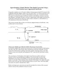
(Fig. 1). This paleogeography, which is also known as
“Pangea A”, results from simple closure of the Atlantic so that Africa
M. Domeier et al. / Tectonophysics 514–517 (2012) 14–43
lies to the south of Europe and is juxtaposed with the eastern seaboard
of North America, and South America lies to the south of North
America. Yet, even before plate tectonics gained general acceptance,
nascent alternatives to this model were being formulated. Alexander
du Toit, best-known as an early promulgator of Wegener's ideas of
continental drift, treated Gondwana and Laurussia as independent,
in contrast to the unified and internally rigid Pangea of Wegener (du
Toit, 1937). Fundamentally, it is this challenge to the model of a single,
largely static landmass that the following arguments adhere; and,
invariably, the alternative reconstructions return to the general
supercontinental boundaries of du Toit (Irving, 2004).
2.2. Initial paleomagnetic tests
Carey (1958) improved upon the schematic reconstruction of
Wegener (1922) through a semi-quantitative “orocline analysis”,
which involved the closing of ocean basins through continental rotations
that straightened curved mountain belts. Interestingly, one of
the most prominent features introduced in Carey's treatise, a hypothetical
intra-continental shear zone called the Tethyan Shear System,
anticipated a series of similar structures later invoked to reconcile
global paleomagnetic data; we shall return to this shortly. While
some aspects of Carey's synthesis are now recognized as invalid, the
resulting reconstruction was effectively identical to Wegener's, but,
importantly, comparatively free of distortion (Fig. 2). For example,
Carey (1958) verified the actuality of the South American–African
continental margin congruence by means of movable spherical tracings
on a globe, countering criticism that the fit was only apparent
or an artifact of projection. Using the very few paleomagnetic data
from North America and Europe available at the time (which, moreover,
predated routine laboratory demagnetization and principal
component analysis), Carey (1958) and Irving (1958) were able to
show the first-order veracity of the reconstruction of the northern
continents (Laurussia) for the late Paleozoic and early Mesozoic.
With respect to the global reconstruction, however, Jeager and Irving
(1957) discovered a disparity in the position of the late Paleozoic–
early Mesozoic paleopoles of Laurussia and Australia, and concluded
that the reconstruction was in need of revision (Fig. 2). Similarly,
Carey (1958) noted a wider scatter in the Carboniferous and Permian
paleopoles (from both Laurussia and Gondwana), relative to those
from the Triassic and Jurassic. He interpreted this to be an indication
that the reconstruction was only appropriate for the latter periods,
and that additional (late Paleozoic) strain would need to be reversed
in order to reach the true paleogeography of the late Paleozoic.
Although preliminary, these early observations represent the
inception of the conundrum that has persisted to the present day:
the paleomagnetic data appear irreconcilable with the conventional
15

16 M. Domeier et al. / Tectonophysics 514–517 (2012) 14–43
paleogeographic model of Pangea for late Paleozoic–early Mesozoic
time.
2.3. The Tethys Twist
30˚N
Equator
30˚S
Fig. 1. Late Paleozoic assembly of Pangea (“Urkontinent”), according to Wegener (1922), the classic “A-type” reconstruction. Note the prominent distortion of India, among other
more minor flaws.
In the early 1960s, students of the University of Utrecht, under the
supervision of R.W. Van Bemmelen, began conducting routine paleomagnetic
investigations during their graduate studies. From the
course of this work it was discovered that Permian rocks from Alpine
Europe repeatedly yielded paleomagnetic poles that were incompatible
with those derived from stable (interior) Europe (Dietzel, 1960;
Van der Lingen, 1960; Van Hilten, 1962; 1964; De Boer, 1963; 1965;
Guicherit, 1964; and references therein). Although it was initially
L A U R A S I A
G O N D W A N A
Paleopoles
Laurasia
Australia
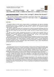
Fig. 2. Semi-quantitative Pangea reconstruction of Carey (1958), generated in part by
his “orocline analysis”. Distortion was minimized through the use of spherical tracings,
but Carey ultimately abandoned a completely distortion-free approach to achieve a
good fit. Superposed are the late Paleozoic–early Mesozoic paleomagnetic data of
Jeager and Irving (1957), showing the already-then recognized disparity between
data from Laurussia (Laurasia) and Gondwana (Australia).
From Irving (2004) with permission from American Geophysical Union.
considered plausible that these “anomalous” results were discordant
due to insufficient averaging of secular variation, an internal consistency
among them became apparent as the number of studies grew,
and this seemed to imply a common tectonic origin for the anomalous
poles. The Permian paleomagnetic directions from Alpine Europe
were consistently steeper than those determined from rocks from
the stable interior; the inclinations from Alpine Europe ranged from
−20° (northeastern Spain) to −30° (northern Italy), vs. the expected
range of −5° to +5° extrapolated from stable Europe (Fig. 3). The
smallest theoretical displacement of Alpine Europe that could explain
the observed anomalous inclinations was immediately recognized as
untenable, as it would require the region to occupy the same space
as northern Europe during the Permian. It was also regarded as implausible
that Alpine Europe had drifted northward from the southern
hemisphere, as the declinations were approximately southdirected,
in agreement with the concomitant Kiaman Reversed Superchron
(~318–265 Ma). Drift from the Southern-Hemisphere would
have been accompanied by a requisite ~180° rotation, necessitating
that the original (Permian) magnetizations were acquired in a normal
polarity field, in violation of the Kiaman Reversed Superchron.
Instead, De Boer (1963; 1965) and Van Hilten (1964), recognizing
the longitude indeterminacy of paleomagnetic data, argued that Alpine
Europe was far-traveled, originating 4500+km to the east of
its present location (near present-day Pakistan), where the −20°/
−30° paleoisoclines, extrapolated from stable Europe, intersected
the Tethyan mobile belt (Fig. 4). Building on the conceptual idea of
a Tethyan Shear System (Carey, 1958) and the Indian Ocean “megaundations”
of Van Bemmelen (see Van Bemmelen, 1966), Van
Hilten (1964) and De Boer (1965) postulated that Alpine Europe
was transported 4500+km along a dextral megashear between Laurussia
and Gondwana, which ran parallel to their Tethyan margins (see
also Irving, 1967). It was suggested that Alpine Europe was an extension
of Gondwana, and therefore moving in concert with it, until it
was “smeared off” during Alpine orogenesis. Accordingly, the megashear
was determined to be active from Permian to Eocene time
through a comparison of Triassic and Cenozoic paleomagnetic data
from Alpine Europe with that of stable Europe (De Boer, 1965); Van
Hilten (1964) called this ~200 Myr event the “Tethys Twist”.
Subsequent studies of late Mesozoic and Cenozoic tectonics have
demonstrably shown the postulated timing of the Tethys Twist to
be indefensible. More importantly, the underlying paleomagnetic argument
was refuted by later paleomagnetic work, which demonstrated
that the reported Permian reference magnetization directions
(from stable Europe; Fig. 3) were too shallow, due to contamination
by viscous overprints (Zijderveld, 1967). Similarly, successive

+20
paleomagnetic work in northern Italy demonstrated that the Permian
inclinations from this region, as reported by Van Hilten (1964) and De
Boer (1965), were too steep (Zijderveld et al., 1970). Using the more
reliable stable European paleomagnetic results of Zijderveld (1967),
Hospers and Van Andel (1969) showed that there was no longer a
statistically significant difference between the inclinations measured
M. Domeier et al. / Tectonophysics 514–517 (2012) 14–43
-9
-18
-3
-5
+6
-1
-3
+10
-7
-22
-9
-14 -20 -9
-31
-36
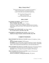
Fig. 3. Permian isocline map redrafted after Van Hilten (1964) and De Boer (1965). The circles represent locations of paleomagnetic study: the values denote the mean inclination
and the arrows portray the mean declination as measured in rocks from these locations. The dashed line separates Alpine Europe (filled circles) from stable interior Europe (open
circles). The Permian isoclines were determined from the stable European results, which are in stark disagreement with the neighboring inclinations from Alpine Europe. Later work
showed both populations of results to be in need of improvement (see text). With permission from Elsevier.
Permian Isocline
0
-10
-20
-30
-35 -48
from rocks in Alpine Europe vs. the expected inclinations extrapolated
from reference directions from stable Europe. And so the Tethys
Twist was refuted. Yet, it would be less than a decade before a
renewed model of intra-continental dextral megashear would be proposed
on the grounds of disparate paleomagnetic data between Laurussia
and Gondwana.
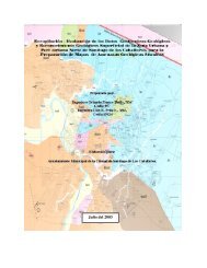
Fig. 4. Extrapolation of Permian isoclines from Fig. 3 along the “Tethyan mobile belt” (yellow zone). Van Hilten (1964) and De Boer (1965) concluded that the anomalous inclinations
observed in Alpine Europe (Fig. 3), here denoted as solid shapes with blue outlines, must have been transported along a dextral megashear from where the −20° Permian
isocline meets the Tethyan mobile belt (solid shapes with red outlines). The arrows illustrate the inferred dextral sense of motion between Gondwana+ Alpine Europe with respect
to stable Eurasia.
Redrafted from De Boer (1965) and Irving (2004) with permission from American Geophysical Union.
-40
17

18 M. Domeier et al. / Tectonophysics 514–517 (2012) 14–43
3. Quantitative A-type Pangea reconstructions
3.1. Pangea A-1
The first quantitative reconstruction of the Atlantic-bordering
continents was produced by Bullard et al. (1965) by least-squares fitting
of the 500 fathom bathymetric contours of the continental margins,
performed by computer. Modifications to the modern margins,
including the omission of prominent Cenozoic features, such as the
Niger Delta, and the rotation of the Iberian Peninsula to close the
Bay of Biscay, were minimal. The result was a landmark achievement
that illustrated the remarkable congruence of the Atlantic coastlines,
free of relative distortion. Smith and Hallam (1970) applied this technique
to the task of reconstructing Gondwana, which allowed them to
verify and refine the earlier work of du Toit (1937). Being similar in
framework to the conceptual reconstruction of Pangea A (Wegener,
1922), the reconstruction built from the combined parameters of
Bullard et al. (1965) and Smith and Hallam (1970) has become
known as Pangea A-1 (Fig. 5A). Although numerous modifications
have been proposed for the peri-Atlantic fit of the A-1 reconstruction
(Dietz and Holden, 1970; Le Pichon et al., 1977, etc.), they have generally
been minor and the parameters of Bullard et al. (1965) have endured
as the conventional reference. An important exception is the
Euler rotation used to bring Laurussia and Gondwana together
(thereby closing the central Atlantic), which, as noted by Bullard et
al. (1965), is the least well-constrained parameter, due to the nonunique
fit of the central Atlantic continental margins. This illdefined
reconstruction parameter exerts a strong control on the separation
of North and South America (present-day Gulf of Mexico),
which is relatively large in the A-1 reconstruction. By reducing this
continental gap through a modification of the Euler rotation, West
Gondwana can be more tightly fit against southern North America;
we consider the paleomagnetic and geologic consequences of this adjustment
next.
3.2. Pangea A-2
Van der Voo and French (1974) tested the Pangea A-1 fitofBullard
et al. (1965) with late Paleozoic and Mesozoic paleomagnetic data
from North America, Europe, and West Gondwana. Although they
concluded that the fit along the North Atlantic was satisfactory,
according to good agreement among the paleomagnetic poles from
North America and Europe, they reported a distinct and systematic
difference between the late Paleozoic poles of West Gondwana and
Laurussia. Yet, the late Paleozoic APWPs defined by these distinct
pole populations shared a common trend, such that they could be
brought into alignment (although with skewed ages) by a single
~20° clockwise rotation applied to Gondwana, about an Euler pole situated
in the southern Sahara. This rotation effectively closes the Gulf
of Mexico gap in the Pangea A-1 fit, bringing northern South America
into a snug fit with southern North America (Fig. 5B). This modified
A-type reconstruction, which was earlier proposed by Le Pichon and
Fox (1971) and Walper and Rowett (1972) on geologic grounds, is
called Pangea A-2. As discussed by Van der Voo et al. (1976), this
model improves the alignment of late Paleozoic orogenic belts and
provides a more reasonable paleogeographic setting for the Florida
peninsula, but it also complicates any scheme describing the tectonic
evolution of Central America and the Caribbean, as it eliminates the
space for northern Mexico and its neighboring continental blocks
Fig. 5. A comparison of alternative Pangea reconstructions, redrafted after Livermore et
al. (1986). (A) Pangea A-1 of Bullard et al. (1965). (B) Pangea A-2 of Van der Voo and
French (1974). (C) Pangea B of Irving (1977) and Morel and Irving (1981). The (pink)
highlighted regions are not correctly positioned, but we have kept them in their
present-day configuration so as to be comparable with other published illustrations.
With permission from Nature.
A
B
C

(Yucatan, Cuba, etc.) in the Gulf of Mexico. Consequently, most subsequent
central Atlantic reconstructions (Klitgord and Schouten, 1986;
Labails et al., 2010; Lottes and Rowley, 1990) have selected reconstruction
parameters intermediate between the “loose” A-1 fit of
Bullard et al. (1965) and the “tight” A-2 fit of Van der Voo and
French (1974). Nonetheless, the A-1 and A-2 models remain useful
as reference points; the term “Pangea A” will be used as a broad
reference to these models in general.
4. Alternatives to A-type reconstructions
4.1. Pangea B
By the late 1970s there was widespread agreement that the paleogeography
of Early Jurassic time – just prior to the opening of the central
Atlantic – was essentially that of Pangea A. This was perhaps most
convincingly demonstrated by detailed correlations of conjugate sea
floor magnetic anomalies and marine fracture zones (see Klitgord
and Schouten, 1986), but Early Jurassic paleomagnetic data were
also shown to be in good agreement with Pangea A. However, the relevance
of this paleogeography in earlier Mesozoic and late Paleozoic
time, from which no in situ seafloor survives, was disputed on paleomagnetic
grounds by Irving (1977), Westphal (1977), Kanasewich et
al. (1978), Morel and Irving (1981), and others later.
Irving (1977) conducted an analysis using Pangea A reference latitudes:
arbitrarily selected reference localities on the margins of the
peri-Atlantic continents that would have been juxtaposed in Pangea
A. If these continents are restored to the paleolatitudes dictated by
their independent paleomagnetic data for a particular time, the reference
latitudes can be compared, and significant relative differences
can be interpreted as a failure of the Pangea A reconstruction for
that specific time. Irving found that the paleomagnetic data agreed
with Pangea A for the Early Jurassic, but could not be rectified with
the model in Permian or Triassic time (Fig. 6a). Specifically, he
found significant disagreement (~10°) between the North American
A B
30
20
10
0
-10
20
10
0
-10
B
?
A
250 200 150
Time (Ma)
M. Domeier et al. / Tectonophysics 514–517 (2012) 14–43
Equator qu
and European reference latitudes for the Triassic, and a significant
and persistent difference in the North American and Gondwanan reference
latitudes for pre-Jurassic time. The relative difference of the
latter implied that, during the Permian and much of the Triassic,
Gondwana must have been farther north, relative to North America,
than its position specified by Pangea A. This was particularly problematic
because, in Pangea A, northwestern Africa is fit snugly against
the eastern seaboard of North America and is juxtaposed with
southwestern Europe, and South America is positioned directly
south of North America; significant northward displacement of
Gondwana, relative to these northern continents, would therefore
result in implausible cratonic overlap (Fig. 6B).
To resolve this problem, Irving (1977) returned to the conceptual
ideas of Van Hilten (1964) and De Boer (1965). Again noting the longitude
indeterminacy of paleomagnetic data, he shifted Gondwana
east, relative to the northern continents, where it could occupy the
more northerly position indicated by the paleomagnetic data, without
resulting in continental overlap. The result is a paleogeography where
Africa is beneath central Europe and South America is juxtaposed
with the eastern seaboard of North America (Fig. 5C). Also, the western
Tethys is replaced with northern Africa and southern North
America is flanked by open ocean. Irving (1977) called this configuration
Pangea B and he considered it relevant from the mid-Carboniferous
to the end Permian/earliest Triassic, in accordance with the
paleomagnetic data. However, the geological and geophysical data
overwhelmingly indicate that the Atlantic opened from Pangea A, requiring
Pangea B to transform to Pangea A during the Middle–Late
Triassic. In a proposal evocative of the Tethys Twist, Irving (1977) hypothesized
that this transformation occurred via a ~3500 km dextral
megashear between Gondwana and Laurussia. He further speculated
that the westward displacement of Gondwana caused North America
to move northward, relative to Europe, thereby causing the difference
he observed in their reference latitudes during the Triassic.
The initial proposal of Pangea B was shortly followed by the paleomagnetic
studies of Kanasewich et al. (1978) and Morel and Irving
Fig. 6. The rationale for Pangea B. (A) Latitude differences (Δλ°) between Pangea A reference latitudes in North America and Gondwana (top panel) and North America and Europe
(bottom panel) as a function of time. The interpreted duration of Pangea B and A are denoted. From Irving (1977) with permission from Nature. (B) Continental overlap that results
if an A-type reconstruction is forced, using the 260 Ma paleomagnetic data of Morel and Irving (1981) to reconstruct Laurussia and Gondwana.
19

20 M. Domeier et al. / Tectonophysics 514–517 (2012) 14–43
(1981), which re-affirmed the general conclusions of Irving (1977),
namely the necessity of Pangea B in the Carboniferous and Permian,
by re-evaluating the agreement between late Paleozoic and Mesozoic
paleomagnetic data from the major continents, when rotated into
different Pangea reconstructions. These conclusions were later reiterated
by Torcq et al. (1997) and, most recently, by Rapalini et al. (2006),
but were based on limited datasets. Torcq et al. (1997) compared an
updated (to 1996) Permo-Triassic paleomagnetic dataset from
Laurussia against a comparatively dated dataset from Gondwana,
which included only two post-1980 results. Notably, with the updated
dataset from North America, they did not detect a significant difference
between the Triassic paleopoles of North America and Europe,
as observed by Irving (1977) and Morel and Irving (1981). The study
of Rapalini et al. (2006) incorporated several additional post-1980
paleopoles from Gondwana, but exclusively from Argentina and
Peru; paleomagnetic data from the other Gondwana blocks were not
included in the analysis, which compared the South American
Permo-Triassic data against the North American APWP of McElhinny
and McFadden (2000).
Westphal (1977) also determined that the paleogeography of the
Permian was effectively that of Pangea B, but arrived at this conclusion
by different means. He performed a spherical harmonic analysis
using Permian paleomagnetic data from Laurussia and Gondwana and
found that he could best align the center of the apparent offset dipoles,
calculated from the data of each landmass, by rotating them
into a Pangea B geometry. Although novel, this analysis must be considered
dubious. A reliable spherical harmonic analysis requires a robust
dataset, ideally one with a global distribution of observations;
the small amount of geographically restricted data utilized in this
study is most certainly inadequate. Additionally, the apparent persistence
of the offset dipole may imply that the Permian paleomagnetic
data used do not constitute a time-averaged field, and therefore may
not be comparable, or representative of the Permian. Finally, the
physical interpretation of the generating field is non-unique; the effects
of an offset dipole can be equally well expressed by a series of
non-dipole fields. Given the latter observation, a persistent “offset dipole”,
if a lasting geomagnetic characteristic, could be a manifestation
of a long-term non-dipole element in the paleomagnetic field, which
calls into question the fundamental assumption implicit in traditional
paleomagnetic reconstructions. We will return to this last point in
Section 5.
4.2. The Intra-Pangean megashear
Pangea B – being built to accommodate the paleomagnetic data –
presents several serious geologic problems. Ross (1979) and Hallam
(1983) showed paleobiogeographic, stratigraphic, and structural evidence
to be in greater accord with Pangea A. The paleontologic argument
includes the recognition of strong faunal affinities among
Permian invertebrates in southern North America and northwestern
South America, and similarities between late Paleozoic flora and
fauna of northern Africa and western Europe–eastern North America,
rather than central Asia. The stratigraphic argument similarly links
comparable late Paleozoic sedimentary facies between southern
North America and northwestern South America, and between northern
Africa and western Europe–eastern North America. However, the
most serious challenge to Pangea B is the structural argument against
it, which cites an absence of evidence for the proposed ~3500 km
dextral megashear in the Triassic. Although it must be emphasized
that an absence of evidence is not equivalent to an evidence of absence,
it does pose a critical question about the validity of the model.
Given the magnitude of the proposed structure, and the irregular geometry
of the plate boundary between Laurussia and Gondwana, it
would be expected that the Pangea B to A transformation would
leave abundant structural relics. Specifically, dextral motion upon
the plate boundary would subject southwestern Europe to regional
transpression, whereas the southern margin of North America would
experience regional transtension, in addition to local expressions of
transpression/transtension along bends in the trace of the shear
zone, or en echelon structures (Hallam, 1983; Smith and Livermore,
1991; Weil et al., 2001). However, as discussed by Hallam (1983)
and Smith and Livermore (1991), the mid-Permian to Middle Triassic
was a tectonically stable interval; evidence for extension in southern
North America or compression in southwestern Europe is minimal.
Oft-referenced in discussions of the Pangean megashear, the conclusions
of Arthaud and Matte (1977), namely that the Laurussia–
Gondwana boundary may have acted as dextral shear zone, are only
applicable to late Paleozoic time — too old to be pertinent to the
Triassic transformation proposed by Irving (1977) and Morel and
Irving (1981) (see also, Gates et al., 1986). Moreover, the displacements
estimated on the principal faults are an order of magnitude
smaller than required by the proposed transformation (Arthaud and
Matte, 1977; Gates et al., 1986; Smith and Livermore, 1991). Finally,
the adoption of Pangea B would require a fundamental reconsideration
of conventional models of late Paleozoic orogenesis, as
the Appalachian–Mauritanide–Variscan belt would have developed
from a very different incipient framework than generally accepted. In
Pangea B, the Ouachita–Marathon margin is open to the Panthalassa,
the Appalachians are juxtaposed with the northern Andes, and the European
Variscan margin is opposite western Africa (Fig. 5C).
4.3. A revision in timing
Beginning with Muttoni et al. (1996), several more recent paleomagnetic
investigations have concluded that while the Carboniferous–
Early Permian paleomagnetic data from Laurussia and Gondwana are
suggestive of a Pangea B paleogeography, the Late Permian–Triassic paleomagnetic
data can be reconciled with Pangea A (Muttoni et al., 2003;
2009, Rakotosolofo et al., 2006). The obvious implication borne from
this conclusion is that the transformation from Pangea B to A must
have been initiated and largely completed within the Permian period,
contrary to the Triassic-age assigned to the event by earlier work (as
discussed above).
The analysis of Muttoni et al. (1996) chiefly differs from the preceding
studies by the use of Permian–Triassic paleopoles from the Southern
Alps as proxy data for West Gondwana, according to the argument that
Adria has acted as an African promontory, already during the late Paleozoic.
Torcq et al. (1997), for example, explicitly omitted the paleomagnetic
data from Adria in their analysis, arguing that the coherence
between Adria and stable Africa was not well-demonstrated (see also
Dercourt et al., 1986; Vai, 2003). Nevertheless, Muttoni et al. (1996)
showed that a mean paleopole compiled from Early Permian results
from the Southern Alps was statistically indistinct from an Early Permian
paleopole compiled from data from West Gondwana. This comparison,
however, is predicated on the reliability of the latter dataset, which is
comparatively old (pre-1980 results, except one pole from 1981) and
of poor quality; indeed its low quality was the stated purpose of using
the Adria data as a proxy. With an Early Permian to Early Jurassic
APWP, built from the merged Southern Alps–West Gondwana datasets,
and the North American APWP of Van der Voo (1993), Muttoni et al.
(1996) concluded that Pangea A was untenable during the Early
Permian; Pangea B was necessary. However, by Late Permian/Early
Triassic time the Pangea A-2 model of Van der Voo and French (1974)
was able to accommodate the data, and by the Late Triassic the A-1
model was permissible (Fig. 7). Thus, they advocated an “evolutionary
model” of Pangea, one in which the supercontinent underwent progressive
internal change.
Following this contribution – and aiming, in part, to address arguments
subsequently raised against it – Muttoni et al. (2003) presented
additional paleomagnetic data from the Southern Alps and
re-affirmed their earlier conclusion that the paleomagnetic evidence
support Pangea B during the Early Permian, but Pangea A during the

lTrm/lTr
lP/eTr
mTr/eTrl
mTr/eTrl
eP
lTrm/lTr
Pangea A-1
lTr/eJ
Pangea A-2
lTr/eJ
lP/eTr
eP
Pangea B
lTr/eJ
lP/eTr
eP
Late Permian. To sidestep the argument that inclination shallowing in
sediments (discussed in Section 6) could have biased the findings of
Muttoni et al. (1996), Muttoni et al. (2003) used only igneous-based
paleomagnetic poles in their analysis. They reiterated the assertion
that Adria has moved in concert with stable Africa since the late
eJ
mTr/eTrl
lP/eTr
eJ
lP/eTr
lTr/eJ
eP
eJ
lTrm/lTr
lP/eTr
eP
eJ
lTr/eJ
Fig. 7. Late Paleozoic–early Mesozoic apparent polar wander paths of Muttoni et al.
(1996) for Laurussia (red) and West Gondwana (blue), according to Pangea A-1, A-2,
and B reconstructions. Muttoni et al. (1996) noted that the models appear to best-fit
the data at different times and proposed an evolution of Pangea from B (Early Permian)
to A-2 (Late Permian–Early Triassic) to A-1 (Late Triassic–Jurassic). Note that the Early
Permian data are strongly discordant in a Pangea A-1 fit, and that the Pangea A-2
reconstruction better fits the trends of the paths, but fails to align mean poles of the
same age. From Muttoni et al. (1996) with permission from Elsevier.
eP
M. Domeier et al. / Tectonophysics 514–517 (2012) 14–43
eJ
Paleozoic, and showed an agreement between Early Permian
volcanic-based paleopoles from the Southern Alps and Morocco.
Again, however, the African poles used for comparison were comparatively
old (pre-1980 results) and of questionable quality. The authors
built a mean Early Permian paleopole for Gondwana by
merging the Southern Alps and Moroccan datasets and, by comparing
this with an igneous-based mean Early Permian paleopole from
Europe, showed that if Pangea were reconstructed according to the
longitude constraints of an A-type model, it would still result in
~1000 km of crustal overlap between West Gondwana and Laurussia.
They further argued that this result was insensitive to zonal nondipole
fields (discussed in Section 5), as the paleomagnetic inclinations
analyzed were from a narrow band of low paleolatitudes from
the same hemisphere.
Bachtadse et al. (2002) and Rakotosolofo et al. (2006) similarly
calculated a mean Early Permian paleopole for Gondwana and, after
comparing it with the mean Early Permian paleopole for Laurussia
(Van der Voo, 1993), concluded that it supported a Pangea B paleogeography.
Rakotosolofo et al. (2006) further claimed that unpublished
Early Triassic paleomagnetic data from southern Peru were compatible
with Pangea A-2, thereby corroborating a Permian-age for the
Pangea B to A transformation, as proposed by Muttoni et al. (1996;
2003).
The broader tectonic and geodynamic implications of a Permianage
megashear were discussed by Muttoni et al. (2003; 2009). In particular,
these authors drew an association between the timing of the
Pangean transformation, the opening of the Neotethys Ocean, and
lithospheric wrenching, basin development, and magmatism in central
Europe and the Southern Alps during the Permian. The hypothetical
plate circuit for Gondwana included a subduction zone to the
south and west (Panthalassa trench), a spreading center to the east
(Neotethys ridge), and the Intra-Pangean dextral megashear to the
north (Fig. 8). Although a Permian megashear is more temporally coincident
with documented dextral activity in Europe (Arthaud and
Matte, 1977; Schaltegger and Brack, 2007) than a Triassic transformation,
the hypothetical motion required still grossly exceeds estimates of
the true net displacement. Furthermore, many Gondwana–Laurussia
boundary zones lack significant structural relics indicative of dextral
strike–slip motion that post-dates Carboniferous–Permian continental
convergence. For example, the prevailing Permian paleostress field in
northern Iberia is N–S compressive (NNE–SSW compressive in paleogeographic
coordinates), reflecting final Variscan deformation due to
the collision of Gondwana and Laurussia (Weil et al., 2001) (Fig. 9A).
This paleostress field precludes significant, Permian-age, ENE–WSW
oriented, dextral shear in the region, which would require WNW–ESE
compressive stress (NW–SE compressive in paleogeographic coordinates)
(Fig. 9B).
4.4. Pangea C
According to the longitude indeterminacy of paleomagnetism,
Pangea B is perfectly acceptable with respect to the data of Irving
(1977) and others, but it is also non-unique. Irving (1977) acknowledged
this, noting that Gondwana could be placed to the west of
North America, or farther to the east than its position in Pangea B,
but he ultimately deemed these alternatives untenable, given the geologic
difficulties already manifest in the “more conservative” Pangea B
model, as discussed above. Despite this, Smith et al. (1981) argued
that Pangea B did not fully conform to the paleomagnetic data, and
presented an alternative paleogeographic model (“Pangea C”) in
which Gondwana is displaced farther east, relative to its position
with respect to Laurussia in Pangea B. In this reconstruction, northern
South America is juxtaposed with southern Europe and Africa is situated
beneath Asia; this affords further space for Gondwana to be
nudged northward to conform to the paleomagnetic data, without
resulting in overlap between continents. Pangea C faces the same
21

22 M. Domeier et al. / Tectonophysics 514–517 (2012) 14–43
North
America
problems as Pangea B, but exacerbated by the greater offset between
Gondwana and Laurussia. For example, if Pangea C is assumed to
transform to Pangea A within either the Permian or the Triassic
(~50 Myr), the requisite ~6000 km displacement must have occurred
at the remarkable average rate of 12 cm yr − 1 . Furthermore, no major
continent borders eastern North America in Pangea C, obliging
advocates of Pangea C to explain the Alleghenian Orogeny in lieu of
continent–continent collision. A variety of similar paleogeographic
permutations of Pangea are obviously permissible according to the
longitude indeterminacy of paleomagnetism, but are ultimately
subject to the same geologic problems.
5. Non-dipole fields
Panthalassa Trench
5.1. A long-term zonal octupole?
In all of the paleomagnetic studies previously referenced, it is implicitly
(or explicitly) assumed that the time-averaged paleomagnetic
field can be approximated by a geocentric axial dipole (GAD). This is
generally a necessary assumption, for without prior knowledge of the
geomagnetic field structure, it is impossible to define a function relating
inclination and latitude. By assuming that the paleomagnetic field
was “always” a GAD, and that rocks can act as high-fidelity magnetic
recorders on geologic timescales, changes in paleomagnetic direction
can be interpreted as tectonic motion (or true polar wander). Thus,
paleomagnetic plate reconstructions are made according to the assumption
that the structure of the paleomagnetic field is perfectly
well-known. Briden et al. (1971) turned this notion on its head.
They took Pangea A-1 to be the true paleogeography of the Permo-
Triassic and assumed that the paleomagnetic discrepancy with this
reconstruction was due to a geomagnetic departure from a GAD.
Comparing the limited data available at the time against theoretical
inclination vs. latitude curves, the authors concluded that the
Permo-Triassic geomagnetic field was, to a first approximation, a
GAD, but that significant axially-symmetric non-dipole contributions
GR
LAURASIA
Europe
Siberia
Urals
Intra-Pangea dextral shear
South
America
Adria
GONDWANA
Africa
Kazhak
stan
triple
junctio n
Antarctica
Jungar
Tarim
Arabia
Paleo-Tethys
Trench
Neo-Tethys
Iran
Ridge
Greater India
Qaidam
Lhasa
North China
Paleo-Tethys
Ocean
Afghanistan
Karakoram
Mongolia
Sibumasu
Australia
South China
Indochina
Panthalassa
Ocean
30°N
were evident. They observed that the theoretical field with the best
visual fit to the data appeared to be a prevailing dipole with a subsidiary
zonal octupole of the same sign. Interestingly, they also observed
a systematic incongruity in the Permian and Triassic inclinations of
Europe and North America (later observed by Roy (1972), Irving
(1977), and Morel and Irving (1981)), which they noted could not
be explained by zonal magnetic fields.
Three decades later, amid revived debate about Pangea reconstructions,
this concept was revisited by Van der Voo and Torsvik
(2001) and Torsvik and Van der Voo (2002). Van der Voo and
Torsvik (2001) analyzed 300–40 Ma paleopoles from North America
and Europe for evidence of zonal non-dipole fields by comparing predicted
and observed paleolatitudes derived from the data. Importantly,
the primary uncertainty in the reconstruction of Laurussia is
orthogonal to the effects of zonal non-dipole fields, so artifacts from
fitting errors were of no significant consequence to their analysis.
Their slope-fitting analysis revealed a consistent departure from the
expectations of a GAD field (wherein predicted=observed paleolatitudes;
yielding a slope of 1) that could be indicative of a long-term
octupole component, representing ~10% of the total geomagnetic
field. The authors demonstrated that by re-calculating paleolatitudes
with a 10% octupole contribution in the late Carboniferous and a
20% contribution in the Late Permian–Early Triassic, Pangea A could
be accommodated without significant continental overlap (Fig. 10).
These conclusions were broadened by Torsvik and Van der Voo
(2002), who conducted a similar analysis on Paleozoic and Mesozoic
paleomagnetic data from Gondwana. Assuming a Pangea A reconstruction,
they built running mean APWP pairs for Laurussia and
Gondwana using several different geomagnetic field structures (varying
octupole contributions; Fig. 11) and measured the great circle difference
between concomitant mean poles for each APWP pair (due to
the paleogeographic position of Gondwana on the south geographic
pole for much of the Paleozoic, they could not apply the linear regression
analysis comparing predicted vs. observed paleolatitudes used
by Van der Voo and Torsvik (2001)). They found it generally
30°
Qiangtang (north Tibet)
Fig. 8. Early Permian Pangea B reconstruction of Muttoni et al. (2009) displaying theoretical plate kinematics. With permission from GeoArabia.
30°S
0°

A
Equator
B
Equator
Fig. 9. (A) Early Permian paleostress field for northern Iberia as determined by Weil et
al. (2001). (B) Paleostress field expected from the hypothetical Intra-Pangean megashear.
Redrafted after Weil et al. (2001) with permission from the Geological Society of
America.
necessary to correct for an octupole contribution to achieve an optimal
fit between the APWPs, but that the relative contribution of this
optimal octupole component was time-varying. The relative contributions
ranged from 20%–0% and generally diminished with time;
the largest values were required in the late Paleozoic–early Mesozoic,
again confirming that Pangea A could not be reconciled with the
uncorrected paleomagnetic data. The authors noted that the late
Paleozoic–early Mesozoic paleomagnetic poles from Gondwana were
dominantly sedimentary-based, whereas the younger paleomagnetic
poles were mostly derived from volcanic rocks. The implication of
this observation is that inclination shallowing could be partly responsible
for the apparently stronger octupole in the late Paleozoic–
early Mesozoic, as it can produce equivalent effects in sediments.
An igneous-only analysis suggested that inclination shallowing was
not significant; but, notably, the data from Gondwana included few
reliable igneous records. We will return to a discussion of inclination
shallowing in Section 6.
5.2. Return to the GAD hypothesis
Paleomagnetism is the only available tool to make quantitative paleogeographic
reconstructions for pre-Cretaceous time. Yet, this
indispensible utility is predicated on the hypothesis of a static (on
time-scales of ~10–100 ka) paleomagnetic field structure, ideally
M. Domeier et al. / Tectonophysics 514–517 (2012) 14–43
(and near-invariably assumed to be) a GAD. As aforementioned, without
prior knowledge of the field structure, inclination cannot be used
to solve for paleolatitude; and for pre-Pangean time this problem cannot
be inverted (as per the approach of Briden et al. (1971)), as the
gross paleogeography has only been established by paleomagnetic
work underpinned by the GAD assumption. Thus, if the GAD hypothesis
is abandoned, so, too, is our confidence in any pre-Pangean paleogeographic
reconstruction derived from paleomagnetic results. It is
prudent, therefore, to consider what persistent bias could manifest
as an apparent octupole contribution; we will consider this in the
next Section (7). Here we will briefly review recent work that suggests
the hypothesis of a GAD may be relevant since the late
Mesoproterozoic.
Analyses of paleomagnetic datasets 0–5 Ma – during which the
contribution of tectonic plate motion is negligible – have demonstrated
that the time-averaged field is approximately a GAD, with a
subsidiary geocentric axial quadrupole representing ~2–5% of the
total field (Johnson et al., 2008; McElhinny, 2004; Valet and
Herrero-Bervera, 2011). Contributions from a persistent zonal octupole
are generally regarded as insignificant (McElhinny, 2004), but
may represent up to 5% of the total field (Johnson and Constable
1997; Johnson et al., 2008; Kelly and Gubbins, 1997). Similarly,
Courtillot and Besse (2004) detected no significant evidence of an
octupole contribution in their analysis of global 0–200 Ma paleomagnetic
data, which they searched for hemispheric inclination antisymmetry,
relative to a synthetic global APWP. Bazhenov and
Shatsillo (2010) devised an approach to investigate the structure of
the paleomagnetic field from paleomagnetic data distributed across
a large single plate and used this method to demonstrate that zonal
non-dipole contributions to the Late Permian paleomagnetic field
were unlikely to exceed ~10% of the total GAD. As previously discussed,
Muttoni et al. (2003) also questioned the evidence of a significant
zonal octupole field in the Early Permian and showed that
paleomagnetic data from a narrow, low paleolatitude band in the
same hemisphere exhibited the same discrepancy the octupole fields
had been invoked to solve; such a distribution of sites should greatly
minimize relative errors introduced by unrecognized octupole fields.
Indeed, Van der Voo and Torsvik (2004) conducted a simpler test for
evidence of an octupole bias in the Permo-Triassic paleomagnetic
data of Western Europe and concluded that the results were ambiguous;
no evidence of an octupole was found in the 280 Ma or
250 Ma data, while the 290 Ma data were consistent with a subsidiary
octupole.
Repeating the paleomagnetic inclination frequency analysis introduced
by Evans (1976) with an updated dataset, Kent and Smethurst
(1998) concluded that the Precambrian and Paleozoic paleomagnetic
fields may have included strong zonal quadrupole and octupole components
(estimated at 10% and 25%, respectively) that diminished
with time. Such a non-dipole field decay was apparent in the analysis
of Torsvik and Van der Voo (2002), where the octupole contribution
needed to optimize the fit between the Laurussian and Gondwanan
APWPs was observed to diminish with time. However, the assumption
of a random paleogeographic sampling that underlies the analysis
of Kent and Smethurst (1998) has been shown to be invalid by
Meert et al. (2003) and McFadden (2004). Moreover, recent comparisons
of Proterozoic paleomagnetic inclinations and climate-sensitive
paleolatitude proxies (Evans, 2006) and normal and reversed paleomagnetic
data from the 1.1 Ga Keweenawan basalts (Swanson-
Hysell et al., 2009) exhibit no remarkable departures from GAD
expectations.
6. Bias in the paleomagnetic record
As an alternative to challenging the conventional paleogeographic
model or the uniformitarian GAD hypothesis, Rochette and
Vandamme (2001) and Van der Voo and Torsvik (2004), among
23

24 M. Domeier et al. / Tectonophysics 514–517 (2012) 14–43
30˚N
Equator
30˚S
GAD model
30˚N
Equator
30˚S
Late Permian-Early Triassic (c. 250 Ma)
G3=0.1
30˚N
Equator
30˚S
G3=0.2
Fig. 10. Permissible Pangea reconstructions (i.e. those that do not require significant continental overlap) according to 250 Ma paleomagnetic data from Van der Voo and Torsvik
(2001), assuming different geomagnetic field configurations. G3 =strength of zonal octupole field relative to an ideal dipole. Pangea A is permissible at 250 Ma if an octupole
contribution of 20% is assumed.
From Van der Voo and Torsvik (2001) with permission from Elsevier.
Fig. 11. Late Paleozoic–Mesozoic APWPs for Laurussia (black) and Gondwana (gray) constructed according to different assumed paleomagnetic field structures (i.e. including a
varying octupole contribution). G3=strength of zonal octupole field relative to an ideal dipole. The late Paleozoic–early Late Triassic interval exhibits a good-fit with an assumed
G3 of 20%, but the fit of the later Mesozoic poles clearly worsens, suggesting that the G3 contribution (if any) may be time-variant.
From Torsvik and Van der Voo (2002) with permission from John Wiley and Sons.

others, have explicitly suggested that the discrepancy between the
late Paleozoic–early Mesozoic paleomagnetic data of Laurussia and
Gondwana could simply be a manifestation of bias in the paleomagnetic
data. We use the term bias rather than error to denote a systematic
quality; random errors, which are invariably present in any
paleomagnetic dataset, are eliminated through the tiered treatment
and averaging of data. With respect to the gross paleogeography of
the late Paleozoic–early Mesozoic, the most corruptive data bias is
that which is equatorially anti-symmetric, as Pangea straddles the
equator during this time. As discussed above, an unrecognized subsidiary
zonal octupole field can impart an anti-symmetric bias to
paleomagnetic data, but it is not the only phenomenon capable of
such. Indeed, the inclination shallowing of sediments inherently
leads to an anti-symmetric bias, and can produce near-identical
results to those of an octupole field (Fig. 12). Less intuitively, systematic
errors in age assignment or unrecognized overprints or remagnetizations
can yield a similarly anti-symmetric bias, albeit under
specific circumstances. In the following, we explore each of these
potential sources of bias in more detail, with a specific focus on
their possible contributions to the late Paleozoic–early Mesozoic
paleomagnetic discrepancy.
6.1. Inclination shallowing
Examples of sedimentary inclination shallowing have been welldocumented
in a variety of natural settings and rock-types (Arason
and Levi, 1990; Bilardello and Kodama, 2010a,b,c; Celaya and
Clement, 1988; Garces et al., 1996; Gilder et al., 2003a; Iosifidi et al.,
2010; Kent and Tauxe, 2005; Tan et al., 2007; Tauxe and Kent, 1984;
Zijderveld, 1975) and by numerous laboratory re-deposition experiments
(Anson and Kodama, 1987; Deamer and Kodama, 1990; King,
1955; Levi and Banerjee, 1990; Lovlie and Torsvik, 1984; Mitra and
Tauxe, 2009; Sun and Kodama, 1992; Tauxe and Kent, 1984; van
Vreumingen, 1993). The bias appears to affect some sedimentary
magnetic records which are defined by a depositional remanent magnetization
(DRM) or a post-depositional remanent magnetization
(pDRM). In the case of the former, the bias arises from the settling
and compaction of inequant magnetized grains or sedimentary flocs
-30
-20
Apparent Paleolatitude
-10
90
80
70
60
50
40
30
20
10
M. Domeier et al. / Tectonophysics 514–517 (2012) 14–43
in the gravitational field, which may overcome the vertical torque applied
to the particles by the geomagnetic field. The shallow inclination
bias of a pDRM is imparted by post-depositional compaction,
wherein the long-axes of magnetic particles are preferentially rotated
toward the horizontal plane, perhaps by riding passively on larger
plate-like clays to which they are adsorbed. Interestingly, Rochette
and Vandamme (2001) and Tan and Kodama (2002) have suggested
that even a chemical remanent magnetization (CRM), potentially acquired
millions of years after deposition, could “inherit” a shallow inclination
bias by developing along the depositional/compacted fabric
of the host rock, or by mimicking the fabric via alteration of preexisting
grains; an early acquired CRM could also be subject to active
compaction-driven shallowing.
Due to the great diversity of sediment characteristics and depositional
conditions, in addition to the assortment of specific mechanisms
by which a magnetization may acquire a shallow inclination
bias, the magnitude of the bias in sedimentary rocks is variable. Yet,
the bias can be expressed by a very simple relationship between the
local geomagnetic field inclination (I f) and the acquired inclination
(=the measured inclination, Im), namely that of King (1955):
tan (I m)=f tan (I f), where f is the shallowing coefficient, which can
range from 0 (complete shallowing) to 1 (no shallowing) (Fig. 12).
For a given value 0bfb1, this relationship implies that the greatest inclination
bias will occur at mid-latitudes, whereas no value f>0 can
modify the inclination at the equator or poles (where the inclination
is horizontal and vertical, respectively). According to the compilation
of Bilardello and Kodama (2010a), f values from magnetitedominated
sedimentary rocks have been found to range from 0.54
to 0.79, with a mean of 0.65, whereas hematite-dominated sedimentary
rocks have yielded f values from 0.4 to 0.83, with a mean of 0.59.
The minimum f values equate to maximum inclination errors of ~17°
(at λ=|34°|) for magnetite and ~25° (at λ=|38°|) for hematite. In a
normal (reverse) polarity field, inclination error is negative (positive)
in the northern hemisphere and positive (negative) in the southern
hemisphere, thus it is inherently anti-symmetric about the equator
(Fig. 12). Obviously, then, paleomagnetic errors due to inclination
shallowing can be exacerbated by comparing biased directions from
the two hemispheres.
0
0 10 20 30 40 50 60 70 80 90
-10
-20
-30
Dipole
G3 = 0.1
G3 = 0.2
Real Paleolatitude
Fig. 12. The effects of a zonal octupole field and inclination shallowing on paleomagnetic determinations of paleolatitude. The dashed black line indicates the reference paleolatitude
expected from an ideal dipole (apparent paleolatitude =real paleolatitude). The warm-colored lines illustrate the effects of an increasing octupole contribution: G3=strength of
zonal octupole field relative to an ideal dipole. The cool-colored lines illustrate the effects of increasing inclination shallowing (f =shallowing coefficient, see text). The effects are
highly similar (compare the G3 =0.2 and f =0.6 curves) and most pronounced at mid-latitudes.
f = 0.8
G3 = 0.3
f = 0.6
f = 0.4
25

26 M. Domeier et al. / Tectonophysics 514–517 (2012) 14–43
Inclination shallowing is particularly ruinous in that it is generally
undetectable from routine paleomagnetic analysis. In studies conducted
on one homogeneous formation, or on similar lithologic
units, many, if not all, sample inclinations may be similarly biased,
whereas magnetic declinations are not affected by inclination shallowing.
Two independent methods have been developed to identify
and correct for inclination shallowing, neither of which can generally
be retroactively applied to published paleomagnetic datasets. The
magnetic anisotropy method (Jackson et al., 1991) is built on the premise
that an unbiased magnetic recorder must be effectively magnetically
isotropic. A sedimentary rock subjected to inclination
shallowing, therefore, can be recognized by its departure from magnetic
isotropy. The magnetic anisotropy of a rock is a function of
both the the magnetic anisotropy of the individual particles and the
degree of axial alignment among the particles. If both of these parameters
are quantified, they can be used to correct the inclination of a
sample. Unfortunately, when magnetic anisotropy is quantified in paleomagnetic
studies, which is atypical, it is usually in the form of the
anisotropy of magnetic susceptibility, which is an integrative measure
of all the magnetic sources (including diamagnetic and paramagnetic
contributions), and not exclusively a measure of the orientation of the
remanence carrying particles. Moreover, determining the anisotropy
of individual particles is an especially time-consuming and tricky operation
that is rarely performed (although Bilardello et al. (2011)
show that, for hematite, a mean particle anisotropy value of 1.38
may be reliably assumed because its anisotropy is controlled by
magnetocrystalline forces). The alternative approach to eliminating
inclination bias, the so-called “elongation–inclination” (E/I) method
(Tauxe and Kent, 2004), assumes that the distribution of directions
in datasets that perfectly capture the full expression of secular
variation will exhibit a latitude-dependence that is time-invariant.
This latitude-dependence is due to the non-linear relationship
between directions and virtual geomagnetic poles (VGPs): as VGP
populations are commonly assumed to be circularly symmetric, the
distribution of directions cannot be circular, except at very highlatitudes.
The distribution of directions faithfully mapped from a
circular distribution of VGPs will be elliptical, with the long axis
oriented along the meridional (up–down) plane (Fig. 13A); the
elongation of this elliptical distribution is latitude dependent, reaching
a maximum at the equator. By contrast, a distribution of directions
that have been subjected to inclination shallowing will be
“squashed”, so that the observed elongation is less than expected,
or, alternatively, greater than expected but re-oriented so that the
elongation is zonal (horizontal) (Fig. 13B). Thus, by comparing the
A B C
Original Data Shallowed by f=0.4
distribution of measured directions with the predictions of a statistical
paleosecular variation model, inclination shallowing can be
detected and reversed (Fig. 13C). Interestingly, this technique can
also be used to detect contributions from octupole fields, which
would exaggerate the meridional elongation of directional datasets.
The impediment to this method is the requirement that secular variation
be fully expressed in the directional dataset; Tauxe et al. (2008)
demonstrate that >100–150 independent site-means are necessary
to conduct a meaningful E/I analysis. Such large paleomagnetic datasets
are exceedingly rare, even among recently published studies. It is
possible that the E/I technique can yield reliable shallowing estimates
from smaller datasets (~100 samples), where sampling is stratigraphically
homogenous and the sedimentation rate is not too high
(Bilardello et al., 2011). However, it should be noted that such datasets
do not allow for the elimination of sample-level random error,
which reduces the effectiveness of the E/I technique.
Despite the difficulty in retroactively identifying inclination shallowing
in published results, and the tedious laboratory (for the remanence
anisotropy method) or laborious field (for the E/I method)
work required to rigorously correct for it, headway has recently
been made in the context of late Paleozoic–early Mesozoic paleomagnetism.
Kodama (2009) applied the anisotropy of remanence method
to the Late Pennsylvanian Glenshaw Formation in Pennsylvania and
determined that the magnetite-dominated sequence of limestone
and siltstone had a ~10° shallow inclination bias. Bilardello and
Kodama (2010b) similarly applied this method (although using a different
measurement technique) to Late Mississippian–Early Pennsylvanian
hematite-dominated redbeds in the Canadian Maritimes. They
ascertained that the Shepody and Maringouin Formations had a shallow
inclination bias of ~10° and ~4°, respectively. As discussed by
Bilardello and Kodama (2010b,c), the corresponding corrected
Carboniferous paleopoles place North America farther south, as the
sampling areas were situated in the southern hemisphere at this
time and inclination shallowing acts as a low-paleolatitude bias. This
correction actually worsens the overlap between North and South
America in a Carboniferous Pangea A reconstruction. However, it is
likely that if the North American sedimentary-based Carboniferous
paleopoles are biased by inclination shallowing, so, too, are the paleopoles
from Gondwana. Furthermore, because West Gondwana was situated
at mid-latitudes during the mid-to-late Carboniferous, a set of f
values, comparable to those from the North American results, would result
in a greater inclination error (Fig. 12). In considering the maximum
possible effects of inclination error on the Carboniferous reconstruction
of Pangea, Bilardello and Kodama (2010c) employed the minimum
Elongation
2.6
2.4
2.2
2.0
1.8
1.6
1.4
1.2
f=1
1.0 10 15 20 25 30 35 40 45 50 55
Inclination
Fig. 13. Illustration of the Elongation/Inclination (E/I) technique for identifying and correcting a shallow inclination bias in a sedimentary-based paleomagnetic record. (A) Data
generated from paleosecular variation model TK03.GAD at λ =20°. (B) Data from (A) after shallowing by f=0.4; note that the direction of elongation in the distribution of
data-points has changed from north–south (up–down) to east–west (horizontal) as a consequence of shallowing. (C) Finding the best match to the theoretical E/I curve of
Tauxe and Kent (2004) (black dashed line) by assuming different f values and evaluating the change to the data (red line). The best fit, where the red and black lines intersect,
is found to be f=0.4.
f=0.4

observed f values to correct the sedimentary-based results from
Gondwana, and found that Pangea A could easily be accommodated.
The E/I method has been successfully applied to Late Triassic/Early
Jurassic continental sedimentary sequences in North America and
Greenland (Kent and Olsen, 2008; Kent and Tauxe, 2005). Kent and
Tauxe (2005) examined the paleomagnetic records from the Dan
River, Newark, and James Land basins and showed that they have average
inclination errors of ~4°, 10°, and 15°, respectively; these correspond
to average paleolatitude errors of ~2°, 6°, and 14°. Kent and
Olsen (2008) similarly demonstrated that paleomagnetic inclinations
from the Hartford basin have an average shallow inclination bias of
~14° (~8° error in paleolatitude). In both studies, the corrected inclinations
were found to be in closer accord with the paleomagnetic
data from proximal and concomitant igneous rocks, as well as with
the paleolatitudes implied by regional paleoclimate data. Although
these corrections pertain to magnetizations too young to be directly
applicable to the paleogeographic problem of interest here, they importantly
affirm the presence of a pervasive shallow inclination bias
in typical clastic sedimentary rocks. The Late Carboniferous to Triassic
(320–200 Ma) paleomagnetic record from North America, for example,
is dominated by results derived from such rocks; in the compilation
of Torsvik et al. (submitted for publication) they constitute 60 of
the 72 paleomagnetic poles from this interval. The E/I method has
also been applied to an Early Permian result from Brazil (Brandt et
al., 2009) and to Carboniferous results from Ukraine (Meijers et al.,
2010), which yielded paleolatitude corrections of ~1–5°. However,
the dataset of Meijers et al. (2010) does not meet the requisite
~100 site/sample means necessary for a rigorous E/I analysis (they
used b100 specimens), and the corrections may thus be unreliable.
Because paleomagnetic results derived from sedimentary sequences
have not been routinely subjected to tests for a shallow inclination
bias, the extent of the bias in any given APWP is difficult to
estimate. Kent and Irving (2010) side-stepped this problem in their
construction of a Triassic through Paleogene APWP for North America
by excluding all sedimentary-derived paleomagnetic poles that were
not explicitly checked/corrected for inclination error. Correspondingly,
the paleolatitudes that they determined for North America were
higher than those calculated from other APWPs, especially those
dominated by results derived from sedimentary rocks. Unfortunately,
very few igneous-based paleomagnetic results exist for the Early and
Middle Triassic, so Kent and Irving (2010) began their analysis at
230 Ma (they retained only one pre-Late Triassic paleomagnetic
pole in their dataset). To correct for shallow inclination bias in the paleomagnetic
records of earlier time, when igneous-based and
inclination-corrected sedimentary poles are scarce, it is necessary to
make some assumptions. Torsvik et al. (submitted for publication) assumed
an average shallowing coefficient of f=0.6 for all clastic sedimentary
sequences and showed an improved agreement in the
APWPs of Laurussia and Gondwana through the late Paleozoic–early
Mesozoic by correcting for it. In a preceding study, Rochette and
Vandamme (2001) concluded that an average shallowing coefficient
of f=0.5 could reconcile the paleomagnetic poles from Laurussia
and Gondwana in a Pangea A-type fit. To verify the veracity of these
average shallowing estimates, in lieu of direct diagnostic tests,
Domeier et al. (2011b) conducted a VGP distribution analysis on a
set of Permian to Middle Triassic paleomagnetic poles from North
America. Following the aforementioned assumption that unbiased
VGPs should be circularly symmetric, and that the redbeds from
which the poles were derived shared a common shallowing coefficient,
they calculated a range of inclination corrections which would
“unflatten” the observed (elongate) distribution of combined VGPs.
The authors compared the variably-corrected North American APWP
against a new igneous paleomagnetic pole and found a good agreement
with the use of shallowing coefficient f=0.54, which falls between
the assumed values of Rochette and Vandamme (2001) and
Torsvik et al. (submitted for publication).
M. Domeier et al. / Tectonophysics 514–517 (2012) 14–43
6.2. Age bias
Pangea consistently drifted northward (~8 cm/yr) during the late
Paleozoic–early Mesozoic (Steinberger and Torsvik, 2008; Torsvik et
al., submitted for publication; Fig. 14). It is obvious, therefore, that a
paleomagnetic pole from this time interval with an erroneous age assignment
can be expected to generate an error, in the sense that a
predicted paleolatitude for the erroneous age will differ from what
it should be. However, a globally uniform age bias would result only
in absolute paleolatitude errors, where no relative differences would
be detectable in the paleomagnetic poles of correctly restored continental
blocks. Instead, paleomagnetic discrepancies will arise from
regional age bias, such as that arising from systematic errors in intercontinental
correlation. For example, the significant difference in the
Triassic paleopole positions of North America and Europe (restored to
Laurussia) observed by Irving (1977) and Morel and Irving (1981)
has been recognized as an artifact of intercontinental correlation
error (Kent and Tauxe, 2005, Livermore et al., 1986).
To explain the observed late Paleozoic–early Mesozoic paleomagnetic
discrepancy between Laurussia and Gondwana in terms of an
age bias, there must be a hemispheric disparity in the age estimate errors
(i.e. a hemispheric bias). For example, the age estimates from
Laurussia could be erroneously young, relative to the (approximately
correct) age estimates from Gondwana. In other words, a comparison
of (relatively) old paleomagnetic data from Laurussia and (relatively)
young paleomagnetic data from Gondwana will result in a paleogeographic
overlap of the landmasses, due to their common and progressive
northward drift through late Paleozoic–early Mesozoic time. For
example, Rochette and Vandamme (2001) argued that the paleomagnetic
discrepancy observed by Torcq et al. (1997) in their 244 Ma Atype
reconstruction was due to a hemispheric age bias; the 244 Ma
pole of Laurussia was weighted by Permian-age poles, whereas the
244 Ma pole of Gondwana was weighted by Late Triassic-age data
(or even Cretaceous age data; see next section). This disparity
would act to drive the apparent 244 Ma paleolatitudes of Laurussia
and Gondwana toward one another, resulting in continental overlap
if an A-type reconstruction is maintained. Rochette and Vandamme
(2001) concluded that an A-type reconstruction was permissible in
the Triassic, according to the results of Torcq et al. (1997), if the
244 Ma pole of Gondwana was compared with the 214 Ma pole of
Laurussia (which may be more equivalent in true age).
Age (Ma)
Era
Period
Continental Mass Centre
(Latitude)
200
220
240
M e s o z o i c
J. Triassic
260
POLAR
280
300
320
340
P a l e o z o i c
Permian Carboniferous
TROPICAL
Fig. 14. Paleolatitude of the center-of-mass of Pangea in late Paleozoic–early Mesozoic
time, as determined by Torsvik et al. (submitted for publication), showing a steady
(~8 cm/yr) northward drift. Center-of-mass is determined from the mean weighted
latitude of all continents at any given time and is independent of longitude.
Simplified from Torsvik et al. (submitted for publication).
27
360

28 M. Domeier et al. / Tectonophysics 514–517 (2012) 14–43
More generally, Van der Voo and Torsvik (2004) revealed the
presence of an age bias in the Permian paleomagnetic record of stable
Europe, by comparing several mean 250 Ma and 280 Ma paleopoles,
calculated from populations of data with varying age estimate reliability
(Fig. 15). For both intervals, they found that the mean paleopoles
derived from data with higher-quality age estimates yielded
higher European paleolatitudes, which suggests that the low-quality
age estimates may be biased toward younger dates. Unfortunately,
in applying their highest age quality filter, the pole-set of Van der
Voo and Torsvik (2004) was reduced from six poles to one (83%
rejected) at 250 Ma, and from 27 poles to three (89% rejected) at
280 Ma. These drastic reductions in pole quantity prevent such a filter
from being routinely applied, especially to less ample or lowerquality
paleomagnetic datasets, such as those from Gondwana. In
this respect, an age bias can be one of the most challenging datapathologies
to deal with, as only meticulous attention to newly published
or re-assessed age estimates and timescale revisions can resolve
unrecognized and enduring age disparities. Fortunately, the
marked improvements in isotopic dating over the previous decades
have allowed age estimates to be made (or revised) with increasing
precision and reliability, so that recent paleopole compilations are
much less corrupted by relative age errors than older datasets.
6.3. Contaminated magnetizations
Secondary magnetizations are well-known in the study of paleomagnetism,
mostly as a nuisance in the form of a minor overprint,
and often parallel to the present day field (PDF). In most cases, the
magnetization of interest, the characteristic remanent magnetization
(ChRM), must be separated from these secondary magnetizations by
demagnetization techniques. If the secondary magnetization is not
completely eliminated (or the ChRM completely isolated), the calculated
ChRM direction will be corrupted by incorporation of the secondary
component(s). Because secondary magnetizations, like a PDF
overprint, can be consistently oriented and regionally/lithologically
pervasive, an unrecognized or incompletely removed secondary
250 ± 10 Ma
280 ± 10 Ma
6 6 1 2 4
magnetization has the potential to significantly bias a paleomagnetic result.
If a consistently-oriented secondary magnetization contaminates
an assemblage of ChRM directions of mixed polarity, the bias may cancel
out, as the normal and reversed directions would be diametrically
modified. Correspondingly, the contamination would then be detectable
by the reversal test, which would reveal the normal and reverse
mean directions to be non-antipodal. However, in an assemblage of
ChRM directions of single polarity, such a bias would not cancel, and a
reversal test would not be applicable. This is relevant to the discussion
at hand, due to the presence of a long interval of reversed polarity
from ~318 to 265 Ma, the Kiaman Reversed Superchron.
Given the low paleolatitude of Laurussia during the late Paleozoic,
a primary Kiaman magnetization contaminated with a normalpolarity
PDF overprint will be biased downward, toward positive inclinations.
The paleogeographic corollary of this bias is an apparent
southward shift of Laurussia. Such a bias would affect Kiaman-age
magnetizations from Gondwana in an identical manner, resulting in
erroneously high southerly paleolatitudes. The effect of a normalpolarity
overprint superposed on a late Paleozoic–early Mesozoic
magnetization of normal polarity would thus result in paleolatitude
estimates for both Laurussia and Gondwana that were too northerly.
Van der Voo and Torsvik (2004) tested the Permian paleomagnetic
data of Europe for an overprint bias by comparing mean 250 Ma
and 280 Ma paleopoles calculated from well-demagnetized vs. poorly
demagnetized data, following the assumption that the poorly demagnetized
data were more likely to be contaminated by PDF overprints
(Fig. 15). For the earlier interval (280 Ma), which falls within the Kiaman,
the European paleolatitude derived from the welldemagnetized
data was 5° higher than the one derived from the poorly
demagnetized results, which supports the contention of a PDF contaminant
in the latter. For the younger, mixed polarity interval
(250 Ma), the poorly demagnetized data yielded a paleolatitude estimate
3° higher than that derived from the well-demagnetized data,
but this analysis was based on very few poles.
Finally, it is worth noting that a complete remagnetization, if
unrecognized as such, can affect a paleomagnetic dataset in the
All poles Age Quality 2-3 Age Quality 3 Demag Code 1-2 Demag Code 3-4
27 12 3 4 23
60 o N
30 o N
Equator
60 o N
30 o N
Equator
Fig. 15. The paleogeographic position of Eurasia at 280 Ma and 250 Ma according to different data selection criteria by Van der Voo and Torsvik (2004). The bold values denote the
number of paleopoles used in each instance to calculate the paleolatitude. For both intervals, the selection of data with the most reliable ages (U–Pb or 40 Ar– 39 Ar methods) results in
a northward shift in the estimated paleolatitude. This can be explained by the assignment of erroneously young absolute ages by the outdated geochronologic methods. Selecting
the most well-demagnetized data similarly results in a northward shift at 280 Ma, which can be explained by a present-day field magnetization contamination in the less welldemagnetized
data. From Van der Voo and Torsvik (2004) with permission from American Geophysical Union.

same manner as an “old-age” bias (where the assigned age is older
than the true age of the magnetization). Where field stability tests
are not applicable, remagnetized units may be difficult to recognize,
especially if the secondary magnetization is not conspicuously different
in orientation from the expected direction. This is especially relevant
to paleomagnetic data from redbeds, which may acquire their
ChRM from a chemical process, millions of years after deposition. As
an example of this potential bias, we return to the critical remarks
of Rochette and Vandamme (2001) on the conclusions of Torcq et
al. (1997). Torcq et al. (1997) used three Moroccan paleomagnetic
poles with estimated ages of 238 Ma in the calculation of the
244 Ma mean paleomagnetic pole for Gondwana, which was then
used in support of an argument for Pangea B. However, Rochette
and Vandamme (2001) noted that in the 50+ sites represented by
these three Moroccan paleomagnetic poles, all site mean directions
have yielded normal polarity (except one dubious result), and the
poles are indistinct from mid-Cretaceous African results. The predominance
of normal polarity could therefore be interpreted as an indication
that the units were remagnetized during the Cretaceous Normal
Superchron, which would imply that the 244 Ma mean paleopole of
Gondwana, as calculated by Torcq et al. (1997), is biased by Cretaceous
data.
7. Approaching resolution
To succinctly summarize the previous sections: the paleomagnetic
data from Laurussia and Gondwana have been repeatedly shown to
be incompatible with a Pangea A-type paleogeography for the late Paleozoic,
and by some accounts, for the Early to Middle Triassic as well.
However, the magnitude and duration of this incongruence have
been diminishing with continued study, a trend which suggests that
it may simply be a long-lived data artifact. Indeed, it has been demonstrated
that several subtle biases may cooperatively act to corrupt the
paleomagnetic dataset in such a way as to drive the apparent paleogeographic
positions of both Laurussia and Gondwana toward lower
latitudes (i.e. toward the equator). This hypothesis is an important
potential solution to this paleomagnetic problem, which otherwise
requires either a fundamental restructuring of Pangea (unsupported
geologically), or adoption of a non-uniformitarian non-dipole geomagnetic
field during the late Paleozoic–early Mesozoic (implicitly
calls into question all prior conclusions from pre-Mesozoic paleomagnetic
work). In the following, we re-evaluate the above hypothesis by
re-calculating and comparing the APWPs of the major peri-Atlantic
continental blocks in light of the most recent paleomagnetic data,
newly refined continental fits, and theoretical inclination shallowing
corrections. As we are here concerned with the first-order fit between
Laurussia and Gondwana, we omit paleomagnetic data from East
Gondwana (Antarctica, Australia, India–Pakistan, Madagascar),
which would otherwise introduce additional uncertainty when
reconstructed to West Gondwana (due to their less-than-perfectly
known reconstruction parameters). However, we note that discrepancies
between late Paleozoic–early Mesozoic paleomagnetic data
from East Gondwana and West Gondwana/Laurussia remain an important
unresolved problem that merits future investigation. One
possibility that already appears to be rather evident is that the paleomagnetic
results obtained from the detrital sedimentary formations
of East Gondwana are very likely in need of inclination-correction.
With a complete absence of results from this interval from Antarctica,
only Australian igneous rocks are – in principle – suitable for
comparisons.
7.1. Data quality
“Data quality” is difficult to evaluate, as it is a subjective measure,
but the use of even a crude quality-criterion can be useful in illuminating
the impact of any bias that may be present in the form of
M. Domeier et al. / Tectonophysics 514–517 (2012) 14–43
unreliable or corrupt data. As an example, we consider the difference
in the APWPs of North America, Europe, and West Gondwana, as constructed
from the updated paleomagnetic dataset of Torsvik et al.
(submitted for publication) (Table 1), relative to those constructed
by Morel and Irving (1981), following the assumption that newer results
are generally of higher quality due to improved laboratory techniques
and analytical treatments. We have elected to use the dataset
of Morel and Irving (1981) because many of the more recent studies
which assert support for Pangea B have focused on a limited interval
of time, such as the latest Permian–earliest Triassic (Torcq et al.,
1997) or the Early Permian (Bachtadse et al., 2002; Muttoni et al.,
2003; Rakotosolofo et al., 2006), rather than considering the complete
late Paleozoic–early Mesozoic time frame of interest here. Because
the quantity and quality of the available paleomagnetic data are highly
variable across this interval, it is important to consider all results in
the context of their temporal neighbors; isolated comparisons can be
seriously misleading, as expounded in our discussion of the potential
sources of bias. Moreover, the conclusions of several of these more recent
studies are predicated on the use of data collected prior to 1980
(as noted in Section 4); this data was already included in the study of
Morel and Irving (1981).
We constructed the APWPs using a 30-Myr moving window, as
was originally done by Morel and Irving (1981), and all APWPs
were rotated into African coordinates, according to Bullard et al.
(1965) (Table 2; Fig. 16). Unfortunately, significant changes in the
reference timescale prevent a direct comparison between specific
mean poles of the “new” and “old” paths, but qualitative comparisons
of their shapes and trends are nonetheless informative. In the newer
APWPs of both North America and Europe there is a clear eastward
shift in the Permian segments, relative to the older paths of Morel
and Irving (1981), and the trend of the Late Permian–Early Triassic
curvature is inverted (Fig. 16A, B). Conversely, the newer path for
Gondwana is displaced west, and slightly north, relative to the older
one. The Permian segments of the Gondwana paths are more congruous
with one another, but the Triassic section of the newer path is
more westward convex. These changes result in greater accord between
the North America–Gondwana and Europe–Gondwana paths
for the Permian–Early Triassic; the great circle distance (GCD) between
the paths is reduced on the order of ~5°–10° for this interval
(Fig. 16D, E), and their trends are visibly more congruent. We again
emphasize that these improvements are free of differences in APWP
construction or continental-reconstruction parameters; they are due
solely to data selection, which in turn is reflective of the impact of
data-quality.
To further consider the reliability of the Torsvik et al. (submitted
for publication) compilation, we have conducted a simple datafiltering
exercise. We re-calculated the APWPs as before, having excluded
all results with ≤29 samples and/or ≤three sites and/or a
global paleomagnetic database DEMAG code of ≤two (Table 1).
While these specific filter thresholds are admittedly arbitrary, smaller
data-sets are less likely to average secular variation, and poorly
demagnetized samples are less likely to be purged of secondary magnetizations,
so the sample/site quantity and DEMAG code parameters
are particularly well-suited for such a quality-filtering exercise. We
elected not to apply any age-quality filters (as per Van der Voo and
Torsvik, 2004), as the datasets of North America and Gondwana still
contain too few high-quality age data for the filtered results to be useful.
Moreover, age reliability was already considered in the pole selection
by Torsvik et al. (submitted for publication). Upon filtering, the
APWPs of North America and Europe change rather little, both exhibiting
a minor northeastward shift in the Late Carboniferous–Early
Permian (Fig. 16C). The APWP of Gondwana becomes less-well defined
with filtering, losing much of its sinuosity, but it does not exhibit
any consistent shift in position. The GCDs between the North
America–Gondwana and Europe–Gondwana APWPs reveal a small
reduction with filtering, supporting the contention that the APWP
29

30 M. Domeier et al. / Tectonophysics 514–517 (2012) 14–43
Table 1
325–195 Ma paleomagnetic poles from Laurussia and West Gondwana, compiled by
Torsvik et al. (submitted for publication). The following criteria were applied in pole
selection: to be included, a pole must (1) have a Q-factor of 3 or greater, (2) be tectonically
coherent with a continental craton (an exception is made for the Colorado
Plateau, where the poles are adjusted by a counterclockwise rotation of 5.4° (Bryan
and Gordon, 1990)), (3) not be remagnetized, and (4) have a reliably known age.
Poles added to or combined from the original compilation are listed in bold. Plat/
Plon=paleopole latitude/longitude. α 95=the semi-angle of the 95% cone of confidence
about the mean magnetization direction (underlined values are A 95, whichisthe95%
cone of confidence about the mean pole). Age=estimated paleopole age in Ma (based
on the timescale of Gradstein et al., 2004). Notes: X (with italicized line)=entry removed
during filtering exercise of Section 7.1. *=corrected for inclination shallowing by f=0.6
in Section 7.3 and Section 8. “i”=inclination shallowing correction applied by original
authors. #=corrected for Colorado Plateau rotation (see above). References: Global
Paleomagnetic Database reference number (Ref no. in: http://www.ngu.no/geodynamics/
gpmdb/) or original reference information.
Formation
Laurussia
North America
Plat Plon α95 Age Notes Reference
Newark volcanics I −63.0 263.1 2.3 197 1702
Connecticut Valley volcanics −65.5 267.5 11.1 197 X 477
Moenave Fm −62.5 251.0 2.8 197 #,i Donohoo-Hurley
et al. (2010)
Hartford Newark basalts
and volcanics
−68.0 268.5 4.0 197 2278
Watchung basalts −63.6 268.7 6.2 197 1339
Hettangian Newark red
beds
−55.6 274.6 6.0 198 * 2312
Piedmont dikes −61.5 234.0 7.9 199 1809
North Mountain basalt −66.4 252.0 10.7 200 1932
Hartford basin −66.6 268.2 3.2 201 i Kent and Olsen
(2008)
Newark Martinsville core −67.8 275.8 5.0 204 i Kent and Tauxe
(2005)
Chinle Group,
Redonda Fm
−58.5 256.9 8.0 204 * 2979
Chinle Fm −58.7 250.9 10.7 204 #,* 2800
Chinle Fm, Redonda Member −57.8 259.3 4.2 204 X,* 152
Newark Martinsville core −64.9 276.6 6.5 204 i Tan et al. (2007)
Newark Weston core −58.1 271.8 2.5 207 i Tan et al. (2007)
Newark Westonville −66.9 267.2 5.0 207 i Kent and Tauxe
(2005)
Passaic Fm, baked
sediments
−65.5 255.1 4.7 211 2791
Passaic Fm −55.6 274.6 5.6 211 * 2312
Chinle Fm −56.6 255.9 3.4 211 #,* 2380
Newark Somerset core −61.7 274.7 4.0 211 i Kent and Tauxe
(2005)
Newark Basin both
polarities
−57.6 269.6 3.0 211 * 1339
Taylor Mountain
−61.4 282.2 5.2 212 Symons et al.
batholith
(2009)
Newark Rutgers core −60.1 277.1 3.1 214 i Kent and Tauxe
(2005)
Manicouagan Structure,
Quebec
−60.1 271.8 7.0 215 434
Manicouagan Structure,
Quebec
−59.0 267.6 10.0 215 X 443
Popo Agie Fm, Chugwater −56.1 276.0 14.0 215 X,* 1334
Ankareh Fm −50.5 267.6 7.8 215 * Weil et al.
(2010)
Chinle Fm, Bull
Canyon Member
−57.4 267.7 5.6 216 * 2380
Newark Titusville core −59.9 279.4 3.2 217 i Kent and Tauxe
(2005)
Chinle, Sangre de Cristo −52.9 282.0 5.1 218 #,* 2979
Dockum Group, Trujillo
and Tecovas Fms
−56.4 276.8 7.7 218 * 2944
Shinarump Member,
Chinle Fm
−59.6 277.5 5.0 220 #,* 2489
Newark Basin,
Lower redbeds
−53.4 281.7 5.0 220 * 2331
Dan River–Danville Basin −58.5 279.5 2.0 221 i Kent and Tauxe
(2005)
Newark Nursery core −60.5 281.6 5.0 221 i Kent and Tauxe
(2005)
Abbott Pluton −48.3 272.3 3.9 221 X 1831
Table 1 (continued)
Formation Plat Plon α95 Age Notes Reference
Newark Princeton core −54.1 285.2 4.0 227 i Kent and Tauxe
(2005)
Agamenticus Pluton −48.4 278.5 3.2 228 1831
Upper Moenkopi drillcore −54.1 288.3 2.5 230 #,X,* 160
Chugwater Fm −45.2 295.4 4.0 230 X,* 1266
Upper Moenkopi Fm −52.5 290.7 3.1 230 #,X,* 159
Moenkopi Fm (upper) −56.5 283.2 4.5 230 #,* 2808
Chugwater Fm −46.1 293.6 3.3 230 * 1271
Moenkopi Fm
(Gray Mountain)
−54.6 284.5 5.0 234 #,* 1221
Moenkopi Fm,
Anton Chico Member
−44.7 301.4 4.9 234 #,* 2979
Combined Moenkopi −57.6 280.3 2.8 234 Com.,* 2489
Moenkopi Fm., CO −55.6 285.8 4.9 234 #,* 571
Moenkopi Fm −41.1 305.6 5.3 234 #,X,* 2632
Combined Red Peak −47.3 294.0 5.8 230 Com.,* 1334
Lower Fundy Group −44.3 271.6 7.2 246 * Symons et al.
(1989)
Dewey Lake Fm −51.0 306.5 5.0 250 * 2303
Bernal Fm −49.9 298.1 8.0 255 #,X,* 2489
Ochoan red beds −54.8 299.3 15.0 258 * 688
Guadalupian red beds −51.5 306.7 5.0 263 * 688
Illinois intrusives −56.3 302.9 3.8 270 Domeier et al.
(2011b)
Downey Bluff sill −53.0 308.7 3.8 272 X Reynolds et al.
(1997)
Hicks Dome breccia −54.8 292.1 8.6 272 X Reynolds et al.
(1997)
Toroweap Fm −51.9 303.0 10.0 277 #,X,* 688
Leonardian subset −51.7 302.1 5.0 277 * 688
Artinskian Pictou
red beds
−42.1 306.5 3.6 280 * 2281
Churchland pluton −33.5 306.3 16.3 282 1264
Fountain and Lykins Fms −44.6 305.3 13.1 283 #,X,* 504
Abo Fm −46.8 304.0 2.1 285 #,* 1311
Piedmont Maficintrusions−38.9 300.8 10.2 289 1527
Upper Casper Fm −50.5 303.0 1.5 291 * 1455
Elephant Canyon Fm −37.5 296.6 5.0 292 #,X,* 671
Cutler Fm, Lisbon Valley −40.1 307.7 7.1 292 #,X,* 1341
Ingelside Fm −43.1 307.9 2.0 292 #,* 1142
Cutler Fm −41.6 300.4 2.0 292 #,X,* 671
Minturn and Maroon Fms −40.1 300.5 2.8 298 #,* 1685
Upper Maroon Fm −55.3 279.8 12.8 299 #,X,* 504
Dunkard Fm −44.1 301.5 3.9 300 * 302
Laborcita Fm −42.1 312.1 2.1 301 * 1311
Wescogame Fm −44.1 303.9 3.4 301 #,* 1311
Lower Casper Fm −45.7 308.6 1.8 303 * 1455
Glenshaw Fm −28.7 299.8 3.1 303 i Kodama (2009)
Riversdale Group −36.0 302.0 6.0 310 * 1110
Shepody Fm, Nova Scotia −29.0 298.3 7.7 317 i Bilardello and
Kodama
(2010b)
Mauch Chunk −22.6 294.4 8.3 320 i Bilardello and
Kodama
(2010c)
Maringouin Fm,
−29.7 296.4 15.3 322 i Bilardello and
Nova Scotia
Kodama
(2010b)
Greenland
Gipsdalen and Fleming
Fjord Fms
−52.7 278.7 5.0 209 i Kent and Tauxe
(2005)
Stable Europe
Kerforne dyke, France −61.0 259.0 7.5 198 2743
Hettangian-Sinemurian
limestone
−55.0 280.0 9.0 201 X 3141
Paris Basin sediments −51.0 285.0 3.0 201 3029
Andesites, Ukraine −50.0 286.4 4.5 204 Yuan et al.
(2011)
Rhaetian sediments,
Germany, France
−50.0 292.0 8.0 208 * 3141
Merci mudstone,
Somerset
−50.0 308.0 5.1 215 * 3311
Sunnhordland dike −50.0 305.0 4.6 221 X Walderhaug
(1993)

Table 1 (continued)
Formation Plat Plon α95 Age Notes Reference
Gipskeuper sediments −49.0 311.0 6.0 226 3141
Taimyr Sills, Siberia −47.1 301.6 2.9 228 Walderhaug
et al. (2005)
Heming limestone, France −54.0 321.0 3.0 234 2411
Musschelkalk carbonates,
Poland
−53.0 303.0 12.0 234 3253
Bunter and Musschelkalk,
Germany
−49.0 326.0 15.0 239 * 158
Upper Buntsandstein,
France
−43.0 326.0 5.0 243 * 1028
Volpriehausen Fm, −49.0 348.2 3.8 246 * Szurlies
Germany
(2004)
Taimyr basalts, Siberia −59.3 325.8 7.8 248 Walderhaug
et al. (2005)
German Trias,
−50.6 345.6 3.3 249 * Szurlies et al.
Lower Buntstein
(2003)
Taimyr Siberian Traps,
Siberia
−59.0 330.0 10.0 250 X 2832
Siberian Traps, Siberia −56.2 326.0 3.3 251 Gurevitch
et al. (2004)
Kotuy River Siberian −52.7 328.4 13.9 251 Pavlov et al.
Traps, Siberia
(2007)
Siberian Traps NSP1 pole −56.4 321.7 2.1 251 Pavlov et al.
(2007)
Sudetes sediments, Poland −50.0 343.0 5.0 251 X,* 3161
Stolbovaya River Siberian −53.3 330.2 5.3 251 Pavlov et al.
Traps, Siberia
(2007)
Big Nirundaiver intrusion, −54.3 323.0 5.0 251 Pavlov et al.
sediments, Siberia
(2007)
Moyero River Siberian −58.5 314.5 2.7 251 Gallet and
Traps, Siberia
Pavlov (1996);
Pavlov et al.
(2007)
Siberian Traps Mean −52.8 334.4 9.7 251 Kravchinsky
recalculated, Siberia
et al. (2002),
recalculated
Dome de Barrot red beds,
France
−46.0 327.0 2.7 255 * 652
Massif des Maures, France −51.0 341.0 4.0 255 * 1408
Late Permian sediments, −45.6 350.2 3.5 260 * Bazhenov
Urals
et al. (2008)
Esterel sediments, France −47.0 331.0 5.0 261 X,* 165
Brive Basin sediments,
France
−49.0 343.0 4.0 261 * 3144
Permian red beds, Lodeve,
France
−53.0 331.0 0.0 264 X,* 1207
Lodeve Basin, France −49.0 334.0 1.5 264 * 1813
Upper Lodeve sandstone,
France
−47.0 336.0 4.6 264 X,* 168
Saxonian red sandstone,
France
−51.0 324.0 4.0 264 X,* 2361
Esterel extrusives, France −51.5 322.0 6.1 264 165
Cracow volcanics B −50.0 344.0 4.1 269 Nawrocki
et al. (2008)
Lunner dikes, Norway −51.0 343.0 2.5 271 Dominguez
et al. (2011)
Lunner dikes, Norway −53.0 344.0 5.9 271 3188, redated
Bohuslan dikes combined,
Sweden
−51.0 345.0 8.6 275 1155
Scania melaphyre dikes,
Sweden
−54.0 352.0 11.0 279 2222
Bohemian quartz porphyry,
Germany
−37.0 341.0 7.0 280 X 3145
Mauchline lavas, Scotland −47.0 337.0 14.0 280 X 3093
Bohemian Massif igneous,
Germany
−42.0 346.0 10.0 280 2356
Oslo volcanics, Norway −47.0 337.0 1.0 281 X 915
Ringerike lavas, Norway −44.6 337.4 13.4 281 1830
Sarna alkaline intrusion,
Sweden
−38.0 346.0 6.9 281 X 1735
Trachytes, Ukraine −49.4 359.7 6.5 283 Yuan et al.
(2011)
Moissey volcanics, France −41.0 352.0 6.7 285 1205
Intrasudetic Basin
volcanics, Poland
−43.0 352.0 3.2 285 3161
North Sudetic Basin
sediments, Poland
−44.0 4.0 5.1 285 X,* 3161
M. Domeier et al. / Tectonophysics 514–517 (2012) 14–43
Table 1 (continued)
Formation Plat Plon α95 Age Notes Reference
Krkonose Basin oil shales,
Czech Republic
−40.0 346.0 2.0 285 X,* 2444
Lower Lodeve sandstone −44.0 350.0 7.7 285 X,* 168
Mount Hunneberg Sill,
Sweden
−38.0 346.0 6.3 285 X 2211
North Sudetic Basin
volcanics, Poland
−42.0 354.0 8.1 285 X 3161
Lodeve Basin, France −42.0 349.0 2.0 285 * 1813
Lodeve B Component,
France
−49.0 342.0 17.0 285 X,* 2454
Intrasudetic basin
sediments, Poland
−37.0 340.0 6.8 285 X,* 3161
Krakow volcanics, Poland −43.0 345.0 7.9 285 X 275
Bohemian red beds,
Czech Republic
−41.0 345.0 4.0 285 X,* 167
Lower Silesia volcanics, −40.0 352.0 13.2 285 X 465,
Poland
recalculated
Exeter Lavas, UK −50.0 330.0 4.0 286 461
Black Forest volcanics, −49.0 356.0 5.9 286 170,
Germany
recalculated
Exeter Lavas, UK −48.0 343.0 10.0 286 X 411,
recalculated
Black Forest rhyolites,
Germany
−42.0 353.0 1.0 286 X 2941
Thuringer Forest
sediments, Germany
−41.5 340.0 5.8 287 X,* 1792
Stabben Sill, Norway −32.0 354.0 2.4 291 X 1540
Saar-Nahe volcanics,
Germany
−41.0 349.0 15.9 291 X 712
Nahe volcanics, Germany −46.0 347.0 13.0 291 X 940
Sudetic Mountain
granitoids, Poland
−42.0 346.0 13.0 293 2446
Great Whin Sill, UK −44.0 339.0 4.8 294 X 585
Hadrian's Wall–Pennines −32.9 347.1 3.5 294 X Liss et al.
Sill and Hett Dike
(Whin Sill), UK
(2004)
Holy Island Sill and −35.4 346.8 6.3 294 X Liss et al.
Dyke (Whin Sill), UK
(2004)
Nideck–Donon volcanics,
France
−47.0 348.0 4.0 294 X 1010
Lower Nideck volcanics,
France
−42.0 348.0 19.0 294 X 174
Cracow volcanics A, −44.0 355.0 4.8 294 Nawrocki
Poland
et al. (2008)
Alnwick Sill, High Green and −47.1 337.1 8.1 294 X Liss et al.
St. Oswalds Chapel Dyke
(Whin Sill), UK
(2004)
Scania dolerites, Sweden −38.0 348.0 6.5 294 2222
Scania dolerite dikes, Sweden −37.0 354.0 11.0 294 2211
Thuringer Forest volcanics,
Germany
−37.1 350.0 7.1 295 X 1792
Silesia volcanics, Poland −43.0 354.0 13.6 296 X 465
Arendal diabase dykes,
Norway
−42.5 339.6 7.1 297 X 175
Ny-Hellesund sills, Norway −39.0 341.0 2.9 297 X 626
Peterhead dyke, Scotland −41.0 342.0 1.3 297 1535
Donets basin, Ukraine −43.0 345.0 3.0 297 X,* Iosifidi et al.
(2010)
Svedlodarsk, Karamysh Fm, −48.4 349.8 2.4 299 X,* Meijers et al.
Donbas
(2010)
Mount Billinger sill, Sweden −31.0 354.0 4.0 299 2211
Donets basin, Ukraine −42.0 359.0 4.0 301 X,* Iosifidi et al.
(2010)
Debaltsevo Donbas, Ukraine −48.2 342.3 2.0 303 X Meijers et al.
(2010)
Wackerfield dyke, England −49.0 349.0 3.0 303 X 180
Queensferry sill, Scotland −38.3 354.0 5.2 305 X 2447
Westphalian–Stephanian
red beds, Czech Republic
−38.0 343.0 9.0 305 X,* 167
Tashkovska Donbas, −38.4 339.5 2.9 312 X Meijers et al.
Ukraine
(2010)
West Gondwana
Amazonia
Anari and Tapirapua
Fms, Brazil
−65.5 250.3 3.8 197 3316
31
(continued on next page)

32 M. Domeier et al. / Tectonophysics 514–517 (2012) 14–43
Table 1 (continued)
Formation Plat Plon α95 Age Notes Reference
French Guyana dikes, Brazil −81.2 235.1 4.0 198 3378
Bolivar dykes, Venezuela −66.9 245.6 4.9 203 X 150
Dolerite dykes, Suriname −82.0 320.0 10.0 232 701
Mitu Group red beds, Peru −71.4 303.6 5.7 249 * 3524
Independencia Group −80.7 7.0 6.6 260 i Rapalini et al.
(2006)
Multiple Fms.,
−81.8 344.2 3.5 280 * Gilder et al.
E. Cordillera, Bolivia
(2003a, b)
Copacabana Group −68.2 321.3 5.2 280 * Rakotosolofo
sediments, Peru
et al. (2006)
Santa Fe Group, Brazil −65.7 330.9 4.1 300 i Brandt et al.
(2009)
Itarare Subgroup,
Tubarao Group, Brazil
−57.0 357.0 11.2 310 X,* 798
Colorado
Mendoza sediments and
volcanics
−51.0 223.0 6.0 195 Iglesia-Llanos
et al. (2006)
Los Colorados Mendoza −81.8 298.3 7.6 216 Vizán et al.
(2004)
Amana Fm, Paganzo Group,
Argentina
−83.0 317.0 7.0 240 X,* 1132
Puesto Viejo Fm
−76.0 312.4 7.3 245 Domeier et al.
Volcanics, Mendoza
(2012)
Puesto Viejo Fm
−87.0 325.0 4.9 245 * Domeier et al.
Sediments, Mendoza
(2012)
Sierra Chica, La Pampa −80.1 348.6 3.3 263 Domeier et al.
(2011a)
Upper Choiyoi Group, −73.7 315.6 4.1 264 Domeier et al.
Mendoza
(2012)
Horcajo, Uspallata Basin,
Argentina
−72.4 264.8 12.0 267 2475
Tambillos, Uspallate
Basin, Argentina
−80.6 308.3 6.5 270 2475
De la Cuesta Fm.,
−77.2 343.6 12.2 275 X,* Spagnuolo
Famatina, Argentina
et al. (2008)
La Colina Fm, Paganzo −80.6 268.8 2.8 283 X,* Geuna and
Escosteguy
(2004)
Middle Paganzo II,
Los Colorados Lower
Beds, Argentina
−59.5 357.5 2.5 283 X,* 620
La Colina Fm, Los
Colorados 1, Argentina
−74.0 313.0 3.1 283 X,* 166
Cerro Colorado −79.3 290.6 11.0 275 * Geuna and
Escosteguy
(2004)
Rincon Blanco, Paganzo −75.0 291.5 6.7 275 Com. Geuna and
Basin, Argentina
Escosteguy
(2004)
La Tabla Fm, Chile −51.0 347.0 5.7 310 1420
Pular and Cas Fms, Chile −57.0 350.0 9.6 310 X 1420
La Colina, Las Mellizas, −67.2 343.7 5.6 310 Geuna et al.
Paganzo, Argentina
(2010)
South Africa
Red sandstone Fm,
Zambia
−68.0 50.5 4.6 222 X,* 323
Cassanje Series, Angola −54.0 80.0 6.0 249 X,* 1960
Karroo Basin −50.9 86.3 7.6 251 X,* De Kock and
Kirschvink
(2004)
K1 Dwyka Varves,
Zimbabwe, Zambia,
Tanzania
−26.5 26.5 5.6 282 X,* 435
Dwyka Group combined −25.0 67.0 12.0 315 * 3489
Meseta
Argana Flows. Morocco −69.2 55.5 6.0 201 Ruiz-Martínez
et al. (submitted
for publication)
Moroccan Intrusives,
Morocco
−71.0 36.0 7.0 201 X 148
Central Atlantic Magmatic −73.0 61.3 19.0 201 Knight et al.
Province, Morocco
(2004)
Taztot Trachyandesite,
Morocco
−38.7 56.8 4.6 273 X 723
Table 1 (continued)
Formation Plat Plon α95 Age Notes Reference
Chougrane red beds,
Morocco
−32.2 64.1 4.7 273 X,* 723
Djebel Tarhat red beds,
Morocco
−24.0 63.8 7.8 273 X,* 1080
Volcanics, Mechra ben Abou, −36.0
Chougrane, Morocco
58.0 20.9 281 X 1859
Somalia
K3 beds, Galula coalfield,
Tanzania
Northwest Africa
Ighrem and Foum Zguid
dykes, Morocco
separation is, at least in part, an artifact of data-quality. However,
the GCD reductions are typically near-negligible, implying that the
remaining separation is due to additional factors, and that the unfiltered
dataset of Torsvik et al. (submitted for publication) is relatively
free of bias due to low-quality data.
7.2. Euler rotations
−46.0 40.0 5.0 257 * 324
−73.0 64.7 4.1 200 Palencia-Ortas
et al. (2011)
Zarzaitine Fm, Algeria −70.9 55.1 2.6 207 * 2932
Abadla Fm., Upper Unit,
Algeria
−29.2 60.0 4.5 273 * 3275
Abadla Fm., Lower Unit,
Algeria
−29.1 57.8 3.6 275 * 3275
Mezarif Basin sediments, −29.3 56.4 3.4 275 * Merabet et al.
Algeria
(2005)
Upper El Adeb Larache Fm,
Algeria
−38.5 57.5 2.8 287 X,* 2540
Lower Tiguentourine Fm,
Algeria
−33.8 61.4 4.1 290 X,* 2728
Merkala Fm., Tindouf −32.4 56.6 2.3 304 * Henry et al.
Basin, Algeria
(1999)
Lower El Adeb Larache
Fm, Algeria
−28.7 55.8 3.5 307 * 2540
Illizi Basin sediments,
Algeria
−28.3 58.9 4.6 309 * 3484
Reggane Basin, Harsi −32.8 55.7 2.0 310 * Derder et al.
Bachir Fm, Algeria
(2009)
Djebel Reouina Fm., −28.4 56.9 1.7 315 * Merabet et al.
Tindouf Basin, Algeria
(1999)
Oubarakat,El-Adeb Larache
Fms, Algeria
−28.2 55.5 4.5 317 * 3481
Reggane Basin, Algeria −26.6 44.7 5.3 320 * 3402
Northeast Africa
Upper Triassic Sediments,
Southern Tunisia
Al Azizia Fm. Combined,
Libya
Jebel Nehoud Ring
Complex, Kordofan,
Sudan
Arabia
Abu Durba sediments,
SW Sinai, Egypt
−54.9 43.3 11.5 222 X,* 3020
−57.0 40.3 6.0 231 Com. 3408
−40.8 71.3 6.0 280 3504
−25.6 64.0 7.2 307 * 2784
In testing various Pangea reconstructions with paleomagnetic data,
the most significant variables are the Euler parameters. Euler rotations
exert a much greater control on the relative positions of the APWPs
than data selection or the choice of APWP construction method, as is
evident in the differences in relative APWP position according to Pangea
A-1, A-2, and B. Yet, the sensitivity of APWPs to Euler parameter
adjustments internal to these general frameworks is often overlooked.
For example, most paleomagnetic tests of Pangea reconstructions
focus only on the fit between Gondwana and Laurussia, implicitly assuming
that the other required Euler parameters are comparatively

Table 2
Reconstruction parameters used or discussed in the text. a,b,c =parameter used in the
construction of apparent polar wander paths in panels (A,B,C) of Fig. 17. European
paleopoles of b220 Ma are rotated to North America according to Euler poles interpolated
from the 220 Ma and 190 Ma reconstruction poles.
North America to Northwest
Africa
Lat Lon Angle
(deg)
Reference
Pangea A-1 ab
67.6 346.0 74.8 Bullard et al. (1965)
Pangea A-2 57.3 339.0 89.0 Van der Voo and French
(1974)
Pangea B 36.2 356.0 77.4 Morel and Irving (1981)
Labails et al. (2010) model c
64.3 345.3 78.1 Labails et al. (2010)
New reconstructions
(inc. corrected, f=0.6)
210 Ma 63.2 352.9 79.0 This paper
220 Ma 63.5 339.8 79.1 This paper
230 Ma 65.3 345.9 75.6 This paper
240 Ma 66.3 346.3 74.1 This paper
250 Ma 66.0 341.1 72.0 This paper
260 Ma 65.9 347.4 75.0 This paper
270 Ma 63.4 345.3 77.9 This paper
280 Ma 65.1 345.5 74.4 This paper
290 Ma 67.9 350.7 70.3 This paper
300 Ma 61.8 335.9 76.6 This paper
310 Ma 59.9 338.2 80.6 This paper
Europe to North America a
88.5 27.7 −38.0 Bullard et al. (1965)
Europe to North America
(310–220 Ma) bc
78.6 161.9 −31.0 Alvey (2009)
Europe to North America
(190 Ma) bc
69.0 154.8 −23.6 Torsvik et al. (submitted
for publication)
Greenland to Europe a
73.0 96.5 22.0 Bullard et al. (1965)
Greenland to Europe bc
65.1 126.1 18.9 Alvey (2009)
South America to Africa a
44.0 329.4 57.0 Bullard et al. (1965)
Amazonia to South Africa bc
50.0 327.5 55.1 Torsvik et al. (2009)
Colorado to South Africa bc
47.5 326.7 57.3 Torsvik et al. (2009)
Arabia to Africa a
36.9 18.0 −6.0 Bullard et al. (1965)
Arabia to South Africa bc
37.1 17.2 −8.9 Torsvik et al. (submitted
for publication)
Northwest Africa to South Africa bc 33.6 26.0 2.3 Torsvik et al. (submitted
for publication)
Northeast Africa to South Africa bc 40.5 298.6 −0.7 Torsvik et al. (submitted
for publication)
Somalia to South Africa bc
9.9 143.0 −0.2 Torsvik et al. (submitted
for publication)
Moroccan Meseta to
Northwest Africa c
29.4 347.9 5.1 Labails et al. (2010)
unimportant. A direct comparison of paleomagnetic poles requires
rotation to a common reference frame, so a comparison of data
from Laurussia and West Gondwana invariably necessitates definition
of at least three Euler parameters: Europe vs. North America,
South America vs. Africa, and Laurussia vs. Gondwana. The first two
parameters are independent of the Pangea A-1, A-2, and (most) B
model distinctions, which are defined by the Laurussia vs. Gondwana
fit. However, significant inaccuracies in either the Laurussia or the
West Gondwana reconstruction could compromise any comparative
analysis of the Pangea models. This is especially true for the Europe
vs. North America parameter, as the paleomagnetic dataset from
Europe is the largest and most reliable for the late Paleozoic–early
Mesozoic. In addition to these first-order variables, important internal
deformation/rotations have been recognized within some continents
(Nuernberg and Mueller, 1991; Torsvik et al., 2008, 2009,
submitted for publication), further compounding the uncertainty in
relative APWP position that may be independent of the Laurussia–
Gondwana fit.
To demonstrate the significance of these parameters, we have
re-calculated the APWPs of Laurussia and Gondwana using the
unfiltered compilation of Torsvik et al. (submitted for publication)
and a series of recently re-determined Euler parameters (Table 2),
and compare them with the same APWPs constructed with the
M. Domeier et al. / Tectonophysics 514–517 (2012) 14–43
conventional Euler parameters of Bullard et al. (1965). Bullard et al.
(1965) treated the continents as rigid plates, so reconstruction of
the APWPs requires only the three rotations listed above (Fig. 17A).
In reconstructing Laurussia according to more recent work, we
adopt the Europe vs. North America parameter of Torsvik et al.
(2006), which is supported by continental lithospheric extension estimates
determined from gravity inversion and seismic refraction
profiles (Alvey, 2009). For West Gondwana, we have elected to use
the reconstruction parameters of Torsvik et al. (2009), which are
based on a relocation of the South Atlantic continent–ocean boundaries
(COBs) by analysis of a variety of geophysical data and geological
information. Following the earlier work of Nuernberg and Mueller
(1991), Torsvik et al. (2009) divide South America into four domains
(Amazonia, Parana, Colorado, and Patagonia) and Africa into five
domains (NW Africa, NE Africa, Somalia, Lake Victoria Block, and
southern Africa), which results in a much improved fit between the
restored COBs. We initially keep the Laurussia vs. Gondwana parameter
constant (retaining that of Bullard et al., 1965), so that any
change in the GCD between the APWPs of Laurussia and Gondwana
in our first comparative analysis must be due solely to the Europe
vs. North America and/or South America vs. Africa parameters
(Fig. 17B). Only minor differences are observed in the APWPs of
Gondwana (as constructed according to Bullard et al. (1965) and
Torsvik et al. (2009), respectively), but the APWPs of Laurussia are
considerably different. The Laurussian path constructed according to
Torsvik et al. (2006) exhibits a significant and consistent shift eastward,
which is due entirely to the difference in the rotation of Europe.
In terms of GCD, the APWPs constructed according to the more recent
parameters are an average of 7° closer than those constructed according
to Bullard et al. (1965) (Fig. 17D); this improvement represents
~46% of the initial difference between the paths.
Turning next to the fit between Laurussia and Gondwana, we compare
the reconstruction parameter of Bullard et al. (1965) with the recently
proposed parameter of Labails et al. (2010) (Table 2), which is
based on a redefinition of the African COB by Sahabi et al. (2004). We
also follow Labails et al. (2010) in applying a minor rotation to the Moroccan
Meseta, relative to NW Africa, which improves the congruence of
the North America–Africa fit. Because we retain an African coordinate
frame, the minor changes to the APWP of Gondwana are due only to
this rotation of the Moroccan Meseta (Fig. 17C). The modified rotation
of Laurussia results in a northeast shift of its APWP, bringing it into closer
proximity with the APWP of Gondwana. This improvement is
reflected in the overall reduction of the GCD between these paths, excepting
the intervals of 290 Ma and 260 Ma, in which the mean poles
are now found to be primarily separated in a North–South direction (orthogonal
to the initial separation). The mean 290 Ma and 260 Ma poles
of Gondwana are both situated at what appear to be short periods of relatively
fast and brief APW; it is likely that these are artifacts of undersampling
(or sampling with a poor temporal distribution: there are no
Gondwana poles in the dataset between 300 and 290 Ma), and we do
not consider these intervals of APWP mis-fit to be critical inadequacies
of the Labails et al. (2010) fit. With the adoption of this fit, the GCD between
mean poles is consistently less than 10°, and the average separation
of 6° is close to the commonly assumed ~5° minimum uncertainty
threshold of paleomagnetism (Fig. 17D). Overall, the adoption of these
new Euler parameters results in a ~58% reduction in the GCD between
the APWPs of Laurussia and Gondwana, relative to our starting point
with the parameters of Bullard et al. (1965), an improvement which is
independent of data selection or other factors.
7.3. Inclination shallowing corrections
The previous exercises have all but demonstrated that the late
Paleozoic–early Mesozoic paleomagnetic Pangea problem is an artifact
arising from the inclusion of low-quality data and usage of coarse and/
or inaccurate Euler parameters. However, after adopting the updated
33

34 M. Domeier et al. / Tectonophysics 514–517 (2012) 14–43
GCD (degrees)
30°S
1
North
America
30°E
30°S
60°S
30° E
30° E
3
West
Gondwana
30
25
20
15
10
5
0
2
Europe
A B C
eP
60°S
lP
mTr
60°S
30°S
lP
lC
mTr
lC
eP
mTr
lTr
lC
lTr
eP
lTr
lP
60° E
60° E
90°E
30°S
30°S
lC eP lP eTr mTr lTr
A
B
C
30°E
30° E
310
220
310
60°S
240
310
260
240
210
280
D North America vs. West Gondwana
5
0
E Europe vs. West Gondwana
310 300 290 280 270 260 250 240 230 220 210
310 300 290 280 270 260 250 240 230 220
Age (Ma)
Age (Ma)
220
230
30°S
GCD (degrees)
280
210
210
260
30° E
280
260
240
30
25
20
15
10
60°S
60° E
60° E
60°S
90°E
30°E
30°S
30°S
30° E
310
310
60°S
240
240
310
260
210
220
230
30°S
290
220
210
210
280
260
30° E
260
240
280
60°S
60° E
60° E
60°S
lC eP lP eTr mTr lTr
A
B
C
90°E
210

30°E
A 31060°E B 310
C
310
220
210
280
260
240
220
210
D
GCD (degrees)
280
20
18
16
14
12
10
8
6
4
2
0
260
240
rotation schemes discussed above and using the most recent compilation
of paleomagnetic data, a significant, albeit smaller, separation remains
between the APWPs for the Late Permian–Middle Triassic
(Fig. 17C). The paleomagnetic datasets of the interval 270–220 Ma contain
a relatively high fraction of sedimentary-based results that have
not been checked/corrected for inclination shallowing, suggesting
that this bias may be prominent for these times (Fig. 18). In the dataset
of Laurussia, 81% (21 of 25) of the constituent paleomagnetic
poles for the 250–230 Ma window are derived from sedimentary sequences
which have not been corrected for inclination shallowing,
the highest proportion in the entire 310–210 Ma interval. In the
dataset of Gondwana, 87% (8 of 9) of the constituent paleomagnetic
poles for the 260–240 Ma window are derived from uncorrected sedimentary
sequences, the highest proportion in its 310–210 Ma
dataset.
A
B
C
30°S
60°S
M. Domeier et al. / Tectonophysics 514–517 (2012) 14–43
30° E
310
220
260
240
210
280
310 300 290 280 270 260 250 240 230 220
Age (Ma)
60° E
280
220
210 10
240
250 50
30°S
60°S
30° E
210
310 10
220
310
260
240
Fig. 17. The significance and influence of Euler rotations as illustrated from a comparative APWP analysis. Panels A–C depict the APWPs of Laurussia (red) and Gondwana (blue)
from the paleomagnetic data in Table 1 and using a moving window of 20-Myr. Mean poles with an A 95 greater than 10° are transparent and poles with a solid symbol are determined
from less than 4 results. (A) APWPs according to the Euler parameters of Bullard et al. (1965). (B) Same as panel (A), but using the Laurussia reconstruction parameters of
Torsvik et al. (2006) and the West Gondwana reconstruction parameters of Torsvik et al. (2009) (the central Atlantic remains reconstructed according to Bullard et al. (1965)). (C)
as in (B), except adopting the central Atlantic reconstruction parameter and the Moroccan Meseta rotation of Labails et al. (2010). The dashed lines in panels (B) and (C) depict the
trend of the APWP from the previous (direct left) panel for comparison. Euler parameters are listed in Table 2. (D) GCD between the APWPs of each panel.
210 10
280
280
220
260
240
210
To check these datasets for the presence of a shallow inclination
bias, we have re-calculated the APWPs after removing all clastic
sedimentary-based poles that are uncorrected for inclination shallowing
(Fig. 19A, B). Accordingly, the 260–240 Ma segment of the
Laurussian APWP shifts to the southeast with this treatment, implying
that the unfiltered dataset is significantly biased by shallow inclinations
in this interval. A less pronounced, but discernable eastward
shift is also observed for the 280–270 Ma interval, in which very recent
results from igneous rocks in Laurussia take on some prominence
(Dominguez et al., 2011; Yuan et al., 2011). Interestingly, a
northeastward shift is observed in the 300–290 Ma interval, due to
the presence of part of Laurentia in the southern hemisphere at that
time, and owing to the valuable inclination-corrected results obtained
by Bilardello and Kodama (2010b). The filtered dataset of Gondwana
is less illuminating, due to the severe reduction in the quantity of
Fig. 16. The importance of data quality as illustrated from a comparative APWP analysis. Columns A, B, and C depict data from Morel and Irving (1981), Table 1, and a filtered version
of Table 1, respectively. The details of the filter are described in the text. Rows 1, 2, and 3 exhibit the APWPs of North America, Europe, and West Gondwana, respectively. Each
APWP is constructed from a 30-Myr moving window, as originally done by Morel and Irving (1981), and rotated into African coordinates according to Bullard et al. (1965).
Mean poles with an A95 greater than 10° are transparent. Mean poles with a solid symbol are determined from less than 4 results. The dashed lines in columns (B) and (C) depict
the trend of the APWP from the previous (direct left) panel for comparison. (D) Great circle distance (GCD) between North America and West Gondwana for columns A, B, and C. (E)
GCD between Europe and West Gondwana for columns A, B, and C. The orange area highlights the improvement (decreased GCD) between results from columns A and B, whereas
the light gray shows intervals of increased GCD.
60° E
30°S
60°S
35

36 M. Domeier et al. / Tectonophysics 514–517 (2012) 14–43
(# of Igneous/corr. sed. poles) - (# of uncorr. sed. poles)
10
5
0
-5
-10
Absolute # of poles
39 35 29 28 28 32 40 58 70 50 28
210 220 230 240 250 260 270 280 290 300 310
Time (Ma)
Fig. 18. Difference calculated as: (1) the number of igneous-based/inclination-corrected
sedimentary-based paleopoles minus (2) the number of uncorrected sedimentary-based
paleopoles (as in Table 1), plotted against time. Time (in Ma) is listed below the central
horizontal axis. Each 10-Myr bin includes data from a 20-Myr moving window (for direct
comparison with the APWPs) centered on the time listed. The absolute number of poles in
each bin is listed above the central horizontal axis.
data; only the 210 Ma and 270 Ma mean poles are built from more
than five results (including several new paleopoles from Argentina
(Domeier et al., 2011a, 2012)), and the average pole quantity for
the 20-Myr moving windows in the 310–210 Ma time-frame is 3.8.
Consequently, the filtered APWP is erratic and unreliable for the interval
of interest (260–230 Ma).
Following the observations from this filtering exercise, and the
identification of a widespread shallow inclination bias in the Permian–Middle
Triassic paleomagnetic data of North America by
Domeier et al. (2011b), we apply an average shallow inclination correction
(f=0.6) to all sedimentary-based results that are prone to inclination
shallowing, as also done by Torsvik et al. (submitted for
publication) (Fig. 19C). The application of this correction to the
APWP of Laurussia appears to under-correct the most strongly biased
intervals (300–290, 250–230 Ma), while coinciding reasonably well
with the filtered mean poles of the remaining intervals (280–260,
220–210 Ma), suggesting that the correction is not excessive. The
change evident in the APWP of Gondwana is more pronounced, partly
due to the greater proportion of sedimentary-based results in its dataset,
but also because Gondwana occupied higher latitudes than Laurussia
during the late Paleozoic–early Mesozoic and the correction
yields the greatest change at mid-latitudes. We are unfortunately unable
to evaluate the pertinence of this correction to the Gondwana
dataset, again due to the low-quality of the filtered APWP, but we
see no reason to expect that the mechanics of shallowing should
have a hemispheric distinction. With the application of this correction,
the average GCD between the APWPs is reduced to 4.7°, and only for
the 310–290 Ma interval is the separation larger than the uncertainty
on the position of the mean Gondwana poles (Fig. 19D). Importantly,
this separation is inverted relative to the original problem; the
300–290 Ma mean poles from Gondwana are west of the equivalent
mean poles from Laurussia, a separation which does not introduce
any unacceptable cratonic overlap, but rather requires a greater distance
between the continents than expected by the Labails et al.
(2010) fit.
It is worth noting that our use of an average inclination correction
is not strictly correct. As aforementioned, f is a function of numerous
variables (grain size, sedimentation rate, post-depositional history,
timing of magnetization acquisition, size and composition of magnetic
carrier, etc.) and will therefore be formation-specific (or even
horizon-specific if such variables are prone to substantial intraformational
change). However, it will be some time before
formation-specific f values are known for the bulk of the (currently
uncorrected) sedimentary-based results. In the absence of these specific
values, application of an average correction likely offers a more
realistic estimate of the true trend of the APWPs, assuming the average
correction is reasonably close to the “true” (and unknown) average
value. In the compilation of Bilardello and Kodama (2010a), the
average f value (from magnetite- and hematite-bearing rocks) is
0.61, with a standard deviation of 0.11, very close to the value of
f=0.6 assumed above. This assumed value is conservative with respect
to the hematite-only average (f=0.59), the values determined
from re-deposition experiments (not included in the compilation of
Bilardello and Kodama (2010a)), and the averaged value calculated
from the VGP distribution analysis of Domeier et al. (2011b). Moreover,
the appropriateness of the applied average value is independently
substantiated by the improved agreement between the
sedimentary-based poles and the igneous-only results in the APWP
of Laurentia, as described above.
To consider what variability could be anticipated in the position of
the APWPs, given the so-far observed variation in f values, we conducted
the following numerical exercise: each sedimentary-based paleomagnetic
pole (without a known f) was corrected with a random
value of f that was drawn from a normal distribution with a mean
of 0.61 and a standard deviation of 0.11. 10-Myr mean poles were
then recalculated with a 20-Myr moving window, as before (igneous-based
poles and previously corrected sedimentary-based poles
were still used in the calculation of mean poles); the procedure was
repeated 1000 times (Fig. 20). The resulting assemblages of reestimated
poles show various distributions, according to the number
of sedimentary-based constituents and the geographic distribution of
their sampling sites. Importantly, the re-estimated poles do not fall
outside the A 95 of the original means (which have a constant assumed
value of f=0.6). This reveals that the variation in formation-specific
(and unknown) f values is relatively unimportant, assuming that the
average correction is close to the “true” average. This is because
pole-specific corrections will only result in local and random mean
pole adjustments, whereas a change in the average correction will result
in a systematic shift of the entire APWP. Given the f values so-far
determined, we contend that the average correction f=0.6 is very
reasonable, and offers a first-order estimate of the true APWP positions.
Future adjustments to the average value and incorporation of
pole-specific f values should be made to these initial estimates.
8. Reconstructions
Having confirmed that the paleomagnetic data can be reconciled
with an A-type Pangea reconstruction through the 310–210 Ma interval,
we now adopt the complimentary approach to reconstructing
Laurussia and Gondwana. We assume the Laurussia vs. Gondwana reconstruction
parameter to be unknown, and instead reconstruct these
landmasses independently according to their paleomagnetic records
at each 10-Myr interval between 310 and 210 Ma. For the reconstruction
parameters internal to Laurussia and Gondwana, we retain those
used in Section 7.2. As longitude is unconstrained by paleomagnetism,
the east–west fitting of Laurussia to Gondwana is determined by visual
inspection in all instances (Table 2). In each case, we attempt to rotate
the landmasses into the closest permissible fit; permissible reconstructions
are those that require no more than a few hundred kilometers of
overlap of modern COBs. A minor overlap of modern COBs is expected
in pre-drift reconstructions, as some extension occurs before continent
break-up. For example, the pre-drift (max. closure) fit ofLabails et al.
(2010) results in ~100 km of COB overlap between North America
and NW Africa. Our delimitation of the central Atlantic COBs follows

A B C
ign*
f =0.6
f =1.0
D
GCD (degrees)
15
10
5
0
ign*
f =0.6
f =1.0
ign*
that of Labails et al. (2010). Following this approach, we can broadly
determine which reconstruction is in closest accord with the paleomagnetic
data for a given interval in the late Paleozoic–early Mesozoic.
We consider the results using both the raw and inclination-corrected
(f=0.6) datasets (Table 3). It is worth re-iterating here that our use
of an average inclination correction is not strictly correct, and the
veracity of the derived reconstructions is ultimately dependent on
the validity of the assumed (average) correction.
If the raw datasets are used in the Late Carboniferous (310 Ma),
reconstruction of the landmasses according to an A-type geometry results
in a large COB overlap (350–550 km) between Laurussia
(specifically eastern North America and Iberia) and NW Africa.
There is also a tight fit between the southern margin of North America
and northern South America, so any small relative sinistral translation
applied to the landmasses (to reduce central Atlantic COB overlap)
310
M. Domeier et al. / Tectonophysics 514–517 (2012) 14–43
f =1.0
f =0.6
Laurussia
West Gondwana
300 290 280 270 260
Age (Ma)
250 240 230 220 210
Fig. 19. Tests and corrections for inclination shallowing in the APWPs of (A) Laurussia and (B) Gondwana. In these panels, the APWPs are built from the data in Table 1 and constructed
using a 20-Myr moving window and the rotation parameters used in Fig. 17C. The dashed black paths are calculated from the raw data (f=1; i.e. no shallowing correction),
the yellow paths are calculated from the same data after removing all poles derived from detrital/clastic sedimentary rocks (leaving results derived from igneous and carbonate
rocks), and the solid colored paths are calculated after applying a blanket inclination correction (f=0.6) to all poles derived from clastic sedimentary rocks. Mean poles with an
A 95 greater than 10° are transparent and poles with a solid symbol are determined from less than 4 results. (C) The solid colored paths (inclination corrected) from panels (A)
and (B) for direct comparison. (D) GCD between the APWPs for each treatment. The vertical dashed lines show the extent of the A 95 error on the Gondwana mean pole estimates,
relative to the GCD between poles of the inclination corrected paths. No statistically distinct separation is observed between 280 and 210 Ma.
will result in cratonic overlap between the Americas, unless Pangea
B is adopted. By the latest Carboniferous (300 Ma), a clockwise
rotation and northward drift of Laurussia, relative to Gondwana,
yields a small paleo-Gulf, ~200–300 km wide, and an excellent fit between
Laurussia and NW Africa (~100–250 km of COB overlap) in an
A-type geometry. At this time, most of Laurussia has drifted into the
northern hemisphere and northwestern Africa is a few degrees
south of the equator. With the application of inclination correction
(for 310–300 Ma), Gondwana is pulled south, away from Laurussia,
resulting in a central Atlantic COB separation of ~200–600 km and a
much larger paleo-Gulf between North and South America (~300–
900 km wide) (Fig. 21). The applied inclination shallowing correction
may therefore be excessive in this interval.
Laurussia and Gondwana continued drifting northward during the
Early Permian (290–270 Ma, Fig. 14). If the raw data are used during
37

38 M. Domeier et al. / Tectonophysics 514–517 (2012) 14–43
Fig. 20. Numerical examination of potential variation in mean pole positions assuming the so-far observed variation in inclination shallowing coefficients (f), as compiled by
Bilardello and Kodama (2010a). The left (right) panel shows re-estimations of the mean pole positions in the APWP of Laurussia (Gondwana). Each panel shows the mean poles
re-estimated by: (1) assigning all uncorrected sedimentary-based paleopoles a value of f drawn randomly from a normal distribution with a mean of 0.61 and a standard deviation
of 0.11, and (2) re-calculating the mean poles by re-averaging the newly-corrected sedimentary-based poles with the igneous-based and previously corrected sedimentary-based
poles. The process is repeated 1000 times (i.e. each mean pole is re-estimated 1000 times). The color scheme was applied to distinguish pole assemblages of different age. The white
poles and their A 95 depict the result using a constant value of f=0.6 (i.e. the mean poles and A 95 from Fig. 19C). The distribution of re-estimated poles is controlled by the relative
number of constituent uncorrected sedimentary-based poles, and the geographic distribution of their sampling sites. Note that none of the re-estimated poles falls outside of the A 95
on the f =0.6 means.
this interval, and an A-type reconstruction is forced, the COB overlap
between Laurussia and NW Africa is large (~300–700 km; greatest at
290 Ma). The North–South America fit is loose at 290 Ma but becomes
increasingly tight with decreasing age (tight at 270 Ma). Again, application
of a small relative sinistral translation between Laurussia and
Gondwana (to relieve some central Atlantic COB overlap) is not
possible due to consequent overlap of the Americas and northern
Gondwana–southern Europe. With inclination correction, a tight to
slightly loose fit (minor to no COB overlap) is achieved between
Laurussia and NW Africa, and a wide paleo-Gulf is observed between
North and South America (~300–900 km) (Fig. 22).
In the Late Permian, Laurussia and Gondwana continue to drift
north and rotate counter-clockwise. Laurussia resides entirely in the
northern hemisphere and NW Africa extends to ~10° N (Fig. 23). At
260 Ma, use of the raw data results in large central Atlantic COB overlap
(~400–700 km) if an A-type geometry is assumed, and the fit between
North and South America remains tight. The inclination
corrected data yield an excellent central Atlantic fit and a wide
paleo-Gulf (Fig. 23). At the Permian–Triassic boundary (250 Ma), an
A-type reconstruction does not appear permissible with the raw
data; it would yield ~500–800 km of COB overlap between Laurussia
and NW Africa and minor cratonic overlap between North and South
America. As before, relative sinistral translation between Laurussia
and Gondwana results in additional overlap until a B-type geometry
is reached. The f=0.6 correction appears to over-compensate for
any bias present in this interval, as it results in a ~350 km separation
of the central Atlantic COBs and the paleo-Gulf exceeds 900 km in
width.
In the Early to Middle Triassic, Laurussia and Gondwana continue
to rotate counter-clockwise, but with minimal northward drift. If an
A-type fit is forced with the raw data, the overlap of the central
Atlantic COBs peaks in this interval (~600–1000 km at 240 Ma), and
significant cratonic overlap between southern North America and
northern South America is again observed. The inclination corrected
data yield a tight COB fit (no overlap) and a wide (~500–800 km)
paleo-Gulf (Fig. 24). In the early Late Triassic (230 Ma), the central
Atlantic COB overlap begins to lessen (~300–700 km) with use of
the raw data; by 220–210 Ma the overlap is further reduced (~300–
600 km). North and South America are tightly fitting to overlapping
throughout the Late Triassic; at 230 Ma this overlap is large (~300–
400 km). With inclination correction, the central Atlantic fit becomes
tight at 230 Ma (minor COB overlap), and the paleo-Gulf is moderately
wide (~400–700 km). For 220 Ma, the corrected data yield a good
fit of the central Atlantic COBs (0–200 km) and a wide paleo-Gulf
(~600 km). No appreciable change is observed with the application
of inclination correction at 210 Ma. Both Laurussia and Gondwana
continue to slowly rotate counter-clockwise through the Late Triassic,
and again begin to drift northward.
In summary, an A-type Pangea reconstruction is permissible for
the entire 310–210 Ma interval if the paleomagnetic data from
Laurussia and Gondwana are corrected for inclination shallowing
(by f=0.6). The specific reconstruction achieved by restoration of

Table 3
Mean 310–210 Ma paleopoles for Laurussia and West Gondwana determined from
Table 1. Mean poles were calculated by means of a 20 Myr moving window at
10 Myr intervals. N=number of paleopoles used in the calculation of the mean pole.
Plat/Plon =paleopole latitude/longitude. All poles are reported in South African coordinates,
using the rotation parameters described in the caption of Fig. 17C (and listed in
Table 2). A 95=the semi-angle of the 95% cone of confidence about the paleopole.
Laurussia and Gondwana according to their independent paleomagnetic
data is similar to the fit ofBullard et al. (1965), but with a
slightly tighter central Atlantic closure, as in the re-assembly of
Labails et al. (2010) (Table 2). Even if the paleomagnetic data are
not corrected for inclination shallowing, an A-type reconstruction is
arguably acceptable for the Late Carboniferous (310–300 Ma), the
late Early to Middle Permian (280–270 Ma), and the Late Triassic
(220–210 Ma). It is only in the Early Permian (290 Ma) and the Late
Permian–Middle Triassic (260–230 Ma) that a forced A-type reconstruction
will result in untenable continental overlap (again, only in
the case that the paleomagnetic data are not corrected for inclination
shallowing). Rather than advocate a rapidly evolving paleogeography
(alternating between Pangea B and A), we contend that this apparent
failure of the A-type model in the Early Permian and Late Permian–
Middle Triassic is a manifestation of a recurring data-artifact.
Following our earlier arguments and the observation that the paleomagnetic
data of the 250–230 Ma interval include a disproportionate
number of results derived from clastic sedimentary rocks (Fig. 18),
we favor the interpretation that this data-artifact equals a shallow inclination
bias.
9. Conclusions
Raw poles Inclination corrected
(f=0.6)
Age
Laurussia
N Plat Plon A95 Plat Plon A95
210 32 −64.2 50.3 2.1 −65.0 54.4 2.0
220 32 −57.8 47.2 2.3 −58.4 51.1 2.4
230 24 −52.3 47.4 2.8 −52.9 50.9 2.9
240 21 −47.4 51.8 4.1 −48.8 56.1 3.7
250 20 −43.8 59.1 3.9 −46.1 61.4 3.2
260 25 −43.0 59.4 2.3 −44.9 61.7 1.9
270 23 −39.1 58.7 2.8 −40.6 60.5 2.9
280 39 −33.2 58.0 2.6 −33.5 58.7 2.6
290 59 −30.8 55.9 2.1 −31.3 56.6 2.1
300 39 −31.0 54.2 2.9 −31.5 55.1 3.0
310 14 −31.7 48.6 6.1 −31.8 49.0 6.3
West Gondwana
210 7 −66.6 61.6 6.0 −67.4 63.9 6.7
220 3 −59.0 53.6 15.9 −55.1 50.0 12.7
230 5 −57.3 54.5 9.5 −54.6 47.3 6.9
240 7 −53.0 62.5 6.7 −51.9 50.4 6.6
250 8 −50.9 65.7 7.3 −48.1 52.1 8.0
260 7 −50.4 62.6 8.5 −48.0 58.5 9.0
270 17 −41.3 62.8 5.7 −40.1 60.6 6.4
280 19 −37.6 60.1 5.8 −35.7 54.9 6.5
290 11 −40.1 56.9 8.0 −38.3 49.0 8.7
300 11 −30.1 56.5 3.7 −26.7 50.6 4.9
310 14 −28.9 56.3 3.3 −25.3 49.6 4.3
A prominent discrepancy between late Paleozoic–early Mesozoic
paleomagnetic data and the most commonly assumed paleogeographic
model of Pangea has been recognized (and has persisted)
for half a century. Three theoretical solutions have been proposed
to resolve this problem: an alternative paleogeographic reconstruction
(notably Pangea B), modification to the GAD hypothesis for (at
least) late Paleozoic–early Mesozoic time, and eradication of, or correction
for, systemic bias in the paleomagnetic data. The former two
hypothetical solutions require substantial revision to widely used
and well-supported models, whereas the latter solution implies
that these models can be reconciled by the use of only the highest-
M. Domeier et al. / Tectonophysics 514–517 (2012) 14–43
Equator
quality data. We have confirmed that the late Paleozoic–early Mesozoic
paleomagnetic data from Laurussia and Gondwana can be reconciled
with a conventional A-type Pangea reconstruction, using an
updated paleomagnetic dataset, recently refined Euler parameters,
and theoretical inclination shallowing corrections. Our review of
previous work and our comparative analysis of APWPs with/without
results derived from clastic sedimentary rocks details support
for the presence of a significant shallow inclination bias in such
rocks. The longitudinally best-fitting reconstruction of Laurussia
and Gondwana, after independently restoring these landmasses to
paleolatitudes determined by their respective paleomagnetic data,
yields a central Atlantic fit similar to the A-type reconstruction of
Bullard et al. (1965). Thesefindings indicate that Pangea can be reconciled
with the paleomagnetic data without requiring serious
paleogeographic re-structuring or non-dipole fields. We have
generated a series of new reconstructions based on our preferred
dataset, which may act as a first-order reference to be updated as
new data and formation-specific inclination shallowing corrections
become available.
Acknowledgments
Late Carboniferous (310 Ma)
Fig. 21. Paleogeographic reconstruction for the Late Carboniferous (310 Ma) using the
inclination corrected data of Laurussia and Gondwana (Table 3) to restore the landmasses
independently. Euler rotations internal to Laurussia and Gondwana are those
used in Fig. 17C. The optimal longitude fit between Laurussia and Gondwana was determined
by visual inspection (Table 2), as paleomagnetic data offer no constraints
on longitude, and was applied by rotating Laurussia along fixed latitude lines, relative
to Gondwana. Arbitrary (undefined) longitudes are depicted at 30° intervals for reference.
The darker brown areas depict (present-day) submerged continental crust which
extends to the continent ocean boundary (COB). The boundaries of the central Atlantic
COBs are taken from Labails et al. (2010). The layers are transparent so that crustal
overlap is evident by darker shades of color. The Piedmont–Florida terrane has been
placed in its present-day position to allow for a comparison between the Atlanticbordering
COBs. In this particular reconstruction (310 Ma), the central Atlantic COBs
are separated by ~200–400 km, indicating that the inclination correction (f =0.6)
may well have been excessive in this interval.
New geochronologic results have been invaluable to our new findings,
and continue to improve the global paleomagnetic data-set; we
acknowledge the recent and ongoing contributions of Eric Tohver and
Bart Hendriks in this respect. We thank Dario Bilardello and an
39

40 M. Domeier et al. / Tectonophysics 514–517 (2012) 14–43
30˚N
Equator
30˚S
Early Permian (280 Ma)
Fig. 22. Paleogeographic reconstruction for the Early Permian (280 Ma) using the inclination
corrected datasets for Laurussia and Gondwana (Table 3). In this reconstruction,
the central Atlantic COBs are closer to each other, relative to Fig. 21, but still separated
by ~100–150 km, so the applied inclination correction may again have been somewhat
excessive. The paleo-Gulf of Mexico is wide, very similar to the A-1 configuration of
Bullard et al. (1965).
anonymous reviewer for their constructive comments. Financial support
for this research was provided by the Norwegian Geological
Survey (NGU), the Center for Advanced Study at the Norwegian
Academy for Science and Letters, the U.S. National Science
Foundation, Division of Earth Sciences (Tectonics Program), and
NSF's Office of International Science and Engineering (Americas
30˚N
Equator
30˚S
Late Permian (260 Ma)
Fig. 23. Paleogeographic reconstruction for the Late Permian (260 Ma) using the inclination
corrected datasets for Laurussia and Gondwana (Table 3). A good fit is observed
between the central Atlantic COBs (minor overlap). A significant paleo-Gulf is still present,
again in agreement with the A-1 model.
Equator
Program), grant EAR-0634807, and is gratefully acknowledged. THT
acknowledges funding from the European Research Council under
the European Union's Seventh Framework Programme (FP7/2007-–
2013)/ERC Grant agreement number 267631.
Appendix A. Supplementary data
Supplementary data to this article can be found online at doi:10.
1016/j.tecto.2011.10.021.
References
30˚N
30˚S
Middle Triassic (240 Ma)
Fig. 24. Paleogeographic reconstruction for the Middle Triassic (240 Ma) using the inclination
corrected datasets for Laurussia and Gondwana (Table 3). A loose fit is observed
in the central Atlantic, and a sizable paleo-Gulf is present between Laurentia
and northern South America. Comparison with Fig. 21 reveals that Pangea has drifted
north and rotated counter-clockwise since the Late Carboniferous.
Alvey, A. (2009). Using crustal thickness and continental lithosphere thinning factors
from gravity inversion to refine plate reconstruction models for the Arctic and
North Atlantic. Ph.D thesis, University of Liverpool, 189 pp.
Anson, G.L., Kodama, K.P., 1987. Compaction-induced inclination shallowing of the
post-depositional remanent magnetization in a synthetic sediment. Geophysical
Journal of the Royal Astronomical Society 88 (3), 673–692.
Arason, P., Levi, S., 1990. Compaction and inclination shallowing in deep-sea sediments
from the Pacific Ocean. Journal of Geophysical Research 95 (B4), 4501–4510.
Arthaud, F., Matte, P., 1977. Late Paleozoic strike–slip faulting in southern Europe and
northern Africa: result of a right-lateral shear zone between the Appalachians
and the Urals. Geological Society of America Bulletin 88 (9), 1305–1320.
Bachtadse, V., Zaenglein, R., Tait, J., Soffel, H.C., 2002. Palaeomagnetism of the Permo/
Carboniferous (280 Ma) Jebel Nehoud ring complex, Kordofan, Central Sudan.
Journal of African Earth Sciences 35 (1), 89–97.
Bazhenov, M.L., Shatsillo, A.V., 2010. Late Permian palaeomagnetism of northern
Eurasia: data evaluation and a single-plate test of the geocentric axial dipole model.
Geophysical Journal International 180 (1), 136–146.
Bazhenov, M.L., Grishanov, A.N., Van der Voo, R., Levashova, N.M., 2008. Late Permian
paleomagnetic data east and west of the Urals. Geophysical Journal International
173, 395–408.
Bilardello, D., Kodama, K.P., 2010a. Rock magnetic evidence for inclination shallowing
in the Early Carboniferous Deer Lake Group red beds of western Newfoundland.
Geophysical Journal International 181 (1), 275–289.
Bilardello, D., Kodama, K.P., 2010b. Palaeomagnetism and magnetic anisotropy of
Carboniferous red beds from the maritime provinces of Canada: evidence for
shallow palaeomagnetic inclinations and implications for North American
apparent polar wander. Geophysical Journal International 180 (3), 1013–1029.
Bilardello, D., Kodama, K.P., 2010c. A new inclination shallowing correction of the
Mauch Chunk Formation of Pennsylvania, based on high-field AIR results:

implications for the Carboniferous North American APW path and Pangea reconstructions.
Earth and Planetary Science Letters 299 (1–2), 218–227.
Bilardello, D., Jezek, J., Kodama, K.P., 2011. Propagating and incorporating the error
in anisotropy-based inclination corrections. Geophysical Journal International
187 (1), 75–84.
Brandt, D., Ernesto, M., Rocha-Campos, A.C., dos Santos, P.R., 2009. Paleomagnetism of the
Santa Fe Group, Central Brazil: implications for the late Paleozoic apparent polar
wander path for South America. Journal of Geophysical Research 114 (B2).
Briden, J.C., Smith, A.G., Sallomy, J.T., 1971. The geomagnetic field in Permo-Triassic
time. Geophysical Journal of the Royal Astronomical Society 23 (1), 101–117.
Bryan, P., Gordon, R.G., 1990. Rotation of the Colorado Plateau: an updated analysis of
paleomagnetic data. Geophysical Research Letters 17, 1501–1504. doi:10.1029/
GL017i010p01501.
Bullard, E., Everett, J.E., Smith, A.G., 1965. The fit of continents around the Atlantic. Philosophical
Transactions of the Royal Society of London 258 (1088), 41–51.
Carey, S.W., 1958. The Tectonic Approach to Continental Drift, in Continental drift, a
symposium, 1956. University of Tasmania, pp. 177–358.
Celaya, M.A., Clement, B.M., 1988. Inclination shallowing in deep sea sediments from
the North Atlantic. Geophysical Research Letters 15 (1), 52–55.
Courtillot, V., Besse, J., 2004. A long-term octupolar component in the geomagnetic
field? 0–200 million years B.P. Timescales of the paleomagnetic field. Geophysical
Monograph 145, 59–74.
De Boer, J., 1963. The geology of the Vicentinian Alps (NE Italy), with special reference
to their paleomagnetic history. Geol. Ultraiectina 11.
De Boer, J., 1965. Paleomagnetic indications of megatectonic movements in the Tethys.
Journal of Geophysical Research 70 (4), 931–944.
De Kock, M.O., Kirschvink, J.L., 2004. Paleomagnetic constraints on the Permian-Triassic
boundary in terrestrial strata of the Karoo Supergroup, South Africa: Implications
for causes of the end-Permian extinction event. Gondwana Research 7, 175–183.
Deamer, G.A., Kodama, K.P., 1990. Compaction-induced inclination shallowing in synthetic
and natural clay-rich sediments. Journal of Geophysical Research 95 (B4),
4511–4529.
Dercourt, J., Zonenshain, L.P., Ricou, L.-E., Kazmin, V.G., Le Pichon, X., Knipper, A.L., et al.,
1986. Geological evolution of the Tethys belt from the Atlantic to the Pamirs since
the Lias. Tectonophysics 123, 241–315.
Derder, M.E.M., Henry, B., Amenna, M., Bayou, B., Djellit, H., Guemache, M.A., Hemmi,
A., 2009. New structural implications for the central Sahara (Algeria), from the
revisited Upper Carboniferous “Hassi Bachir” formation: paleomagnetic constraints.
Tectonophysics 463, 69–76.
Dietz, R.S., Holden, J.C., 1970. Reconstruction of Pangaea: breakup and dispersion of
continents, Permian to Present. Journal of Geophysical Research 75 (26), 4939–4956.
Dietzel, G.F.L., 1960. Geology and Permian paleomagnetism of the Merano region,
province of Bolzano, (N. Italy). Geol. Ultraiectina 4.
Domeier, M., Van der Voo, R., Tohver, E., Tomezzoli, R.N., Vizan, H., Torsvik, T.H.,
Kirshner, J.A., 2011a. New Late Permian constraint on the apparent polar
wander path of Gondwana. Geochemistry Geophysics Geosystems 12. doi:10.1029/
2011GC003616.
Domeier, M., Van der Voo, R., Denny, B., 2011b. Widespread inclination shallowing in
Permian and Triassic paleomagnetic data from Laurentia: support from a shallow intrusive
record and virtual geomagnetic pole distributions. Tectonophysics 511, 38–52.
Domeier,M.,VanderVoo,R.,Tomezzoli,R.N.,Tohver,E.,Hendriks,B.W.H.,Torsvik,
T.H., Vizán, H., Dominguez, A., 2012. Support for an “A-type” Pangea reconstruction
from high-fidelity paleomagnetic records for the Late Permian and Middle Triassic.
Journal of Geophysical Research accepted..
Dominguez, A.R., Van der Voo, R., Torsvik, T.H., Hendriks, B.W.H., Abrajevitch, A., Domeier,
M., Larsen, B.T., Rousse, S., 2011. The 270 Ma paleolatitude of Baltica and its
significance for Pangea models. Geophysical Journal International 186, 529–550.
Donohoo-Hurley, L.L., Geissman, J.W., Lucas, S.G., 2010. Magnetostratigraphy of the
uppermost Triassic and lowermost Jurassic Moenave Formation, western United
States: correlation with strata in the United Kingdom, Morocco, Turkey, Italy and
the eastern United States. Geological Society of America Bulletin 122, 1936–1950.
du Toit, A.L., 1937. Our Wandering Continents: A Hypothesis of Continental Drifting.
Oliver & Boyd, London, UK.
Evans, M.E., 1976. Test of the dipolar nature of the geomagnetic field throughout
Phanerozoic time. Nature 262 (5570), 676–677.
Evans, D.A.D., 2006. Proterozoic low orbital obliquity and axial-dipolar geomagnetic
field from evaporite palaeolatitudes. Nature 444 (7115), 51–55.
Gallet, Y., Pavlov, V., 1996. Magnetostratigraphy of the Moyero River Section (North-
Western Siberia): constraints on geomagnetic reversal frequency during the early
Palaeozoic. Geophysical Journal International 125, 95–105.
Garces, M., Pares, J.M., Cabrera, L., 1996. Further evidence for inclination shallowing in
red beds. Geophysical Research Letters 23 (16), 2065–2068.
Gates, A.E., Simpson, C., Glover III, L., 1986. Appalachian Carboniferous dextral strike–
slip faults: an example from Brookneal, Virginia. Tectonics 5 (1), 119–133.
Geuna, S.E., Escosteguy, L.D., 2004. Palaeomagnetism of the Upper Carboniferous–
Lower Permian transition from Paganzo Basin, Argentina. Geophysical Journal
International 157 (3), 1071–1089.
Geuna, S.E., Escosteguy, L.D., Limarino, C.Ó., 2010. Paleomagnetism of the Carboniferous–
Permian Patquía Formation, Paganzo Basin, Argentina: implications for the apparent
polar wander path for South America and Gondwana during the Late Palaeozoic.
Geologica Acta 8 (4), 373–397.
Gilder, S., Chen, Y., Cogne, J., Tan, X., Courtillot, V., Dongjiang, Sun, et al., 2003a.
Paleomagnetism of Upper Jurassic to Lower Cretaceous volcanic and sedimentary
rocks from the western Tarim Basin and implications for inclination shallowing
and absolute dating of the M-0 (ISEA?) chron. Earth and Planetary Science Letters
206 (3–4), 587–600.
M. Domeier et al. / Tectonophysics 514–517 (2012) 14–43
Gilder, S., Rousse, S., Farber, D., McNulty, B., Sempere, T., Torres, V., Palacios, O., 2003b.
Post-Middle Oligocene origin of paleomagnetic rotations in Upper Permian to
Lower Jurassic rocks from northern and southern Peru. Earth and Planetary Science
Letters 210 (1–2), 233–248.
Gradstein, F.M., Ogg, J.G., Smith, A.G., et al., 2004. A Geologic Time Scale 2004, 610 pp.,
Cambridge Univ. Press, Cambridge U.K.
Guicherit, R., 1964. Gravity tectonics, gravity field, and paleomagnetism in NE-Italy,
with special reference to the Carnian Alps. Geol. Ultraiectina 14.
Gurevitch, E.L., Heunemann, C., Radko, V., Westphal, M., Bachtadse, V., Pozzi, J.P.,
Feinberg, H., 2004. Palaeomagnetism and magnetostratigraphy of the Permian–
Triassic northwest central Siberian Trap Basalts. Tectonophysics 379, 211–226.
Hallam, A., 1973. A Revolution in the Earth Sciences: From Continental Drift to Plate
Tectonics. Clarendon Press, Oxford, UK.
Hallam, A., 1983. Supposed Permo-Triassic megashear between Laurasia and
Gondwana. Nature 301 (5900), 499–502.
Henry, B., Merabet, N.E., Bouabdallah, H., Maouche, S., 1999. New Lower Stephanian paleomagnetic
pole for the Saharan Craton (Merkala Formation, Tindouf Basin, Algeria).
C. R. Acad. Sci. Paris, Sciences de la terre et des planètes 329 (3), 161–166.
Hospers, J., Van Andel, S.I., 1969. Palaeomagnetism and tectonics: a review. Earth-Science
Reviews 5 (1), 5–44.
Iglesia-Llanos, M.P., Riccardi, A.C., Singer, S.E., 2006. Paleomagnetic study of Lower Jurassic
marine strata from the Neuquén Basin, Argentina: a new Jurassic apparent polar
wander path for South America. Earth and Planetary Science Letters 252, 379–397.
Iosifidi, A.G., Mac Niocaill, C., Khramov, A.N., Dekkers, M.J., Popov, V.V., 2010.
Palaeogeographic implications of differential inclination shallowing in Permo-
Carboniferous sediments from the Donets Basin, Ukraine. Tectonophysics 490 (3–4),
229–240.
Irving, E., 1958. Rock Magnetism: A New Approach to the Problems of Problems of
Polar Wandering and Continental Drift, in Continental drift, a symposium, 1956.
University of Tasmania.
Irving, E., 1967. Palaeomagnetic evidence for shear along the Tethys: aspects of Tethyan
biogeography. Publication of the Systematics Association 7, 59–76.
Irving, E., 1977. Drift of the major continental blocks since the Devonian. Nature
270 (5635), 304–309.
Irving, E., 2004. The case for Pangea B, and the Intra-Pangean Megashear. Timescales of
the paleomagnetic field. Geophysical Monograph 145, 13–27.
Jackson, M.J., Banerjee, S.K., Marvin, J.A., Lu, R., Gruber, W., 1991. Detrital remanence,
inclination errors, and anhysteretic remanence anisotropy: quantitative model
and experimental results. Geophysical Journal International 104 (1), 95–103.
Jeager, J.C., Irving, E., 1957. Paleomagnetism and reconstruction of Gondwanaland. C. R.
3rd Congr. Pacific and Indian Ocean Sciences. Imprimerie Officielle, Tananarive,
Madagascar, pp. 233–242.
Johnson, C.L., Constable, C.G., 1997. The time-averaged geomagnetic field: global and
regional biases for 0–5 Ma. Geophysical Journal International 131 (3), 643–666.
Johnson, C.L., Constable, C.G., Johnson, C.L., Constable, C.G., Tauxe, L.W., Barendregt, R.,
Brown, L.L., Coe, R.S., Layer, P.W., Mejia, V., Opdyke, N.D., Singer, B.S., Staudigel, H.,
Stone, D.B., 2008. Recent investigations of the 0- to 5-Ma geomagnetic field
recorded by lava flows. Geochem. Geophys. Geosyst. 9, Q04032http://dx.doi.org/
10.1029/2007GC001696.
Kanasewich, E.R., Havskov, J., Evans, M.E., 1978. Plate tectonics in the Phanerozoic.
Canadian Journal of Earth Sciences 15 (6), 919–955.
Kelly, P., Gubbins, D., 1997. The geomagnetic field over the past 5 million years.
Geophysical Journal International 128 (2), 315–330.
Kent, D.V., Irving, E., 2010. Influence of inclination error in sedimentary rocks on the
Triassic and Jurassic apparent pole wander path for North America and
implications for Cordilleran tectonics. Journal of Geophysical Research 115 (B10).
Kent, D.V., Olsen, P.E., 2008. Early Jurassic magnetostratigraphy and paleolatitudes
from the Hartford continental rift basin (eastern North America): testing for
polarity bias and abrupt polar wander in association with the Central Atlantic
Magmatic Province. Journal of Geophysical Research 113 (B6).
Kent, D.V., Smethurst, M.A., 1998. Shallow bias of paleomagnetic inclinations in the
Paleozoic and Precambrian. Earth and Planetary Science Letters 160 (3–4), 391–402.
Kent, D.V., Tauxe, L., 2005. Corrected Late Triassic latitudes for continents adjacent to
the North Atlantic. Science 307 (5707), 240–244.
King, R., 1955. The remanent magnetism of artificially deposited sediments.
Geophysical Journal International 7, 115–134.
Klitgord, K.D., Schouten, H., 1986. Plate kinematics of the Central Atlantic. In: Vogt, P.R.,
Tucholke, B.E. (Eds.), The Geology of North America: The Western North Atlantic
Region. Geol. Soc. Am, Boulder, CO (USA).
Knight, K.B., Nomade, S., Renne, R., Marzoli, A., Bertrand, H., Youbi, N., 2004. The Central
Atlantic magmatic province at the Triassic–Jurassic boundary; paleomagnetic
and 40 Ar/ 39 Ar evidence from Morocco for brief, episodic volcanism. Earth and
Planetary Science Letters 228, 143–160.
Kodama, K.P., 2009. Simplification of the anisotropy-based inclination correction
technique for magnetite- and haematite-bearing rocks: a case study for the
Carboniferous Glenshaw and Mauch Chunk Formations, North America. Geophysical
Journal International 176 (2), 467–477.
Kravchinsky, A., Konstantinov, K.M., Courtillot, V., Savrasov, J.I., Valet, J.P., Cherniy, S.D.,
Mishenin, S.G., Parasotka, B.S., 2002. Palaeomagnetism of East Siberian traps and
kimberlites: two new poles and palaeogeographic reconstructions at about 360
and 250 Ma. Geophysical Journal International 148, 1–33.
Labails, C., Olivet, J., Aslanian, D., Roest, W.R., 2010. An alternative early opening
scenario for the Central Atlantic Ocean. Earth and Planetary Science Letters 297 (3–4),
355–368.
Le Pichon, X., Fox, P.J., 1971. Marginal offsets, fracture zones, and the early opening of
the North Atlantic. Journal of Geophysical Research 76 (26), 6294–6308.
41

42 M. Domeier et al. / Tectonophysics 514–517 (2012) 14–43
Le Pichon, X., Sibuet, J.-C., Francheteau, J., 1977. The fit of the continents around the
North Atlantic Ocean. Tectonophysics 38 (3–4), 169–209.
Levi, S., Banerjee, S.K., 1990. On the origin of inclination shallowing in redeposited
sediments. Journal of Geophysical Research 95 (B4), 4383–4389.
Liss, D., Owens, W.H., Hutton, D.H.W., 2004. New palaeomagnetic results from the
Whin Sill Complex: evidence for a multiple intrusion event and revised virtual
geomagnetic poles for the Late Carboniferous for the British Isles. Journal of the
Geological Society, London 161, 927–938.
Livermore, R.A., Smith, A.G., Vine, F.J., 1986. Late Palaeozoic to early Mesozoic evolution
of Pangaea. Nature 322 (6075), 162–165.
Lottes, A.L., Rowley, D.B., 1990. Early and Late Permian reconstructions of Pangaea:
Palaeozoic palaeogeography and biogeography. Memoirs of the Geological Society
of London 12, 383–395.
Lovlie, R., Torsvik, T., 1984. Magnetic remanence and fabric properties of laboratorydeposited
hematite-bearing red sandstone. Geophysical Research Letters 11 (3),
221–224.
McElhinny, M., 2004. Geocentric axial dipole hypothesis: a least squares perspective.
Timescales of the paleomagnetic field. Geophysical Monograph 145, 1–12.
McElhinny, M.W., McFadden, P.L., 2000. Paleomagnetism: Continents and Oceans.
Academic Press, San Diego, CA (USA).
McFadden, P.L., 2004. Is 600 Myr long enough for the random palaeogeographic test
of the geomagnetic axial dipole assumption? Geophysical Journal International
158 (2), 443–445.
Meert, J.G., Tamrat, E., Spearman, J., 2003. Non-dipole fields and inclination bias:
insights from a random walk analysis. Earth and Planetary Science Letters 214 (3–4),
395–408.
Meijers, M.J., Hamers, M.F., van Hinsbergen, D.J., van der Meer, D.G., Kitchka, A.,
Langereis, C.G., et al., 2010. New Late Paleozoic paleopoles from the Donbas
Foldbelt (Ukraine): implications for the Pangea A vs. B controversy. Earth and
Planetary Science Letters 297 (1–2), 18–33.
Merabet, N., Henry, B., Bouabdallah, H., Maouche, S., 1999. Paleomagnetism of the
Djebel Reouina Namurian Formation (Tindouf Basin, Algeria). Studia Geophysica
Et Geodaetica 43 (4), 376–389.
Merabet, N., Henry, B., Kherroubi, A., Maouche, S., 2005. Autunian age constrained by
fold tests for paleomagnetic data from the Mezarif and Abadla Basins (Algeria).
Journal of African Earth Sciences 43 (5), 556–566.
Mitra, R., Tauxe, L., 2009. Full vector model for magnetization in sediments. Earth and
Planetary Science Letters 286 (3–4), 535–545.
Morel, P., Irving, E., 1981. Paleomagnetism and the evolution of Pangea. Journal of
Geophysical Research 86 (B3), 1858–1872.
Muttoni, G., Kent, D.V., Channell, J.E.T., 1996. Evolution of Pangea: paleomagnetic
constraints from the Southern Alps, Italy. Earth and Planetary Science Letters
140 (1–4), 97–112.
Muttoni, G., Kent, D.V., Garzanti, E., Brack, P., Abrahamsen, N., Gaetani, M., 2003. Early
Permian Pangea “B” to Late Permian Pangea “A”. Earth and Planetary Science
Letters 215 (3–4), 379–394.
Muttoni, G., Gaetani, M., Kent, D.V., Sciunnach, D., Angiolini, L., Berra, F., et al., 2009.
Opening of the Neo-Tethys Ocean and the Pangea B to Pangea A transformation
during the Permian. GeoArabia 14 (4), 17–48.
Nawrocki, J., Fanning, M., Lewandowska, A., Polechonska, O., Werner, T., 2008.
Palaeomagnetism and the age of the Cracow volcanic rocks (S Poland). Geophysical
Journal International 174, 475–488.
Nuernberg, D., Mueller, R.D., 1991. The tectonic evolution of the South Atlantic from
Late Jurassic to Present. Tectonophysics 191 (1–2), 27–53.
Palencia-Ortas, A., Ruiz-Martínez, V.C., Villalaín, J.J., Osete, M.L., Vegas, R., Touil, A.,
Hafid, A., McIntosh, G., van Hinsbergen, D.J.J., Torsvik, T.H., 2011. A new 200
Ma paleomagnetic pole for Africa, and paleo-secular variation scatter from
Central Atlantic Magmatic Province (CAMP) intrusives in Morocco (Ighrem
and Foum Zguid dykes). Geophysical Journal International 185, 1220–1234.
Pavlov, E., Courtillot, V., Bazhenov, M.L., Veselovsky, R.V., 2007. Paleomagnetism
of the Siberian Traps; new data and a new overall 250 Ma pole for Siberia.
Tectonophysics 443, 72–92.
Rakotosolofo, N.A., Tait, J.A., Carlotto, V., Cardenas, J., 2006. Palaeomagnetic results from
the Early Permian Copacabana Group, Southern Peru: implication for Pangaea
palaeogeography. Tectonophysics 413 (3–4), 287–299.
Rapalini, A.E., Fazzito, S., Orue, D., 2006. A new Late Permian paleomagnetic pole for
stable South America: the Independencia Group, eastern Paraguay. Earth, Planets,
and Space 58 (10), 1247–1253.
Reynolds, R.L., Goldhaber, M.B., Snee, L.W., 1997. Paleomagnetic and 40 Ar/ 39 Ar results
from the Grant intrusive breccia and comparison to the Permian Downeys Bluff
sill — evidence for Permian igneous activity at Hicks Dome, southern Illinois
Basin. U. S. Geological Survey Bulletin 2094-G, 16pp..
Rochette, P., Vandamme, D., 2001. Pangea B: an artifact of incorrect paleomagnetic
assumptions? Annali Di Geofisica 44 (3), 649–658.
Romm, J., 1994. A new forerunner for continental drift. Nature 367 (6462), 407–408.
Ross, C.A., 1979. Late Paleozoic collision of North and South America. Geology 7 (1), 41–44.
Roy, J.L., 1972. A pattern of rupture of the eastern North American–western European
paleoblock. Earth and Planetary Science Letters 14, 103–114.
Ruiz-Martínez, V.C., Torsvik, T.H., van Hinsbergen, D.J.J., Gaina, C., submitted for publication.
Earth at 200 Ma. Earth and Planetary Science Letters.
Sahabi, M., Aslanian, D., Olivet, J., 2004. A new interpretation of the evolution of the
Central Atlantic. Comptes Rendus — Academie Des Sciences. Geoscience 336 (12),
1041–1052.
Schaltegger, U., Brack, P., 2007. Crustal-scale magmatic systems during intracontinental
strike–slip tectonics: U, Pb and Hf isotopic constraints from Permian magmatic
rocks of the Southern Alps. International Journal of Earth Sciences 96 (6), 1131–1151.
Smith, A.G., Hallam, A., 1970. The fit of the southern continents. Nature 225 (5228),
139–144.
Smith, A.G., Livermore, R.A., 1991. Pangea in Permian to Jurassic time. Tectonophysics
187 (1–3), 135–179.
Smith, A.G., Hurley, A.M., Briden, J.C., 1981. Phanerozoic Paleocontinental World Maps.
Cambridge Univ. Press, London, UK.
Snider-Pellegrini, A., 1858. La Création et ses mystères dévoilés. Frank and Dentu, Paris.
Spagnuolo, C., Rapalini, A., Astini, R., 2008. Palaeomagnetic confirmation of Palaeozoic
clockwise rotation of the Famatina Ranges (NW Argentina): implications for the
evolution of the SW margin of Gondwana. Geophysical Journal International
173 (1), 63–78.
Steinberger, B., Torsvik, T.H., 2008. Absolute plate motions and true polar wander in the
absence of hotspot tracks. Nature 452, 620–623.
Sun, W.W., Kodama, K.P., 1992. Magnetic anisotropy, scanning electron microscopy,
and X-ray pole figure goniometry study of inclination shallowing in a compacting
clay-rich sediment. Journal of Geophysical Research 97 (B13) 19,599–19,615.
Swanson-Hysell, N.L., Maloof, A.C., Weiss, B.P., Evans, D.A.D., 2009. No asymmetry in
geomagnetic reversals recorded by 1.1-billion-year-old Keweenawan basalts.
Nature Geoscience 2 (10), 713–717.
Symons, D.T.A., Bormann, R.E., Jans, R.P., 1989. Paleomagnetism of the Triassic red beds
of the lower Fundy Group and Mesozoic tectonism of the Nova Scotia Platform,
Canada. Tectonophysics 164, 13–24.
Symons, D.T.A., Kawasaki, K., McCausland, J.A., 2009. The Yukon–Tanana terrane: part
of North America at 215 Ma from paleomagnetism of the Taylor Mountain batholith,
Alaska. Tectonophysics 465, 60–74.
Szurlies, M., 2004. Magnetostratigraphy; the key to a global correlation of the classic
Germanic Trias; case study Volpriehausen Formation (middle Buntsandstein),
central Germany. Earth and Planetary Science Letters 227, 395–410.
Szurlies, M., Bachmann, G.H., Menning, M., Nowaczyk, N.R., Kaeding, K.C., 2003. Magnetostratigraphy
and high-resolution lithostratigraphy of the Permian-Triassic boundary
interval in central Germany. Earth and Planetary Science Letters 212, 263–278.
Tan, X., Kodama, K.P., 2002. Magnetic anisotropy and paleomagnetic inclination shallowing
in red beds: evidence from the Mississippian Mauch Chunk Formation,
Pennsylvania. Journal of Geophysical Research 107 (B11), 17.
Tan, X., Kodama, K.P., Gilder, S., Courtillot, V., 2007. Rock magnetic evidence for inclination
shallowing in the Passaic Formation red beds from the Newark Basin and a
systematic bias of the Late Triassic apparent polar wander path for North America.
Earth and Planetary Science Letters 254 (3–4), 345–357.
Tauxe, L., Kent, D.V., 1984. Properties of a detrital remanence carried by haematite
from study of modern river deposits and laboratory redeposition experiments.
Geophysical Journal of the Royal Astronomical Society 76 (3), 543–561.
Tauxe, L., Kent, D.V., 2004. A simplified statistical model for the geomagnetic field and
the detection of shallow bias in paleomagnetic inclinations: was the ancient magnetic
field dipolar? Timescales of the paleomagnetic field. Geophysical Monograph
145, 101–115.
Tauxe, L., Kodama, K.P., Kent, D.V., 2008. Testing corrections for paleomagnetic inclination
error in sedimentary rocks: a comparative approach. Physics of the Earth and
Planetary Interiors 169 (1–4), 152–165.
Torcq, F., Besse, J., Vaslet, D., Marcoux, J., Ricou, L.E., Halawani, M., et al., 1997. Paleomagnetic
results from Saudi Arabia and the Permo-Triassic Pangea configuration.
Earth and Planetary Science Letters 148 (3–4), 553–567.
Torsvik, T.H., Van der Voo, R., 2002. Refining Gondwana and Pangea palaeogeography:
estimates of Phanerozoic non-dipole (octupole) fields. Geophysical Journal International
151 (3), 771–794.
Torsvik, T.H., Gaina, C., Steinberg, M., Van der Voo, R., 2006. North Atlantic fits with implications
for the Barents Sea. Norwegian Geol. Survey Industry Report. 17 pp. (confidential).
Torsvik, T.H., Muller, R.D., Van der Voo, R., Steinberger, B., Gaina, C., 2008. Global plate
motion frames: toward a unified model. Reviews of Geophysics 46, 1–44.
Torsvik, T.H., Rousse, S., Smethurst, M.A., 2009. A new scheme for the opening of
the South Atlantic Ocean and the dissection of an Aptian salt basin. Geophysical
Journal International 183 (1), 29–34.
Torsvik, T.H., Van der Voo, R., Preeden, U., Mac Niocaill, C., Steinberger, B., Doubrovine,
P., van Hinsbergen, D.J.J., Domeier, M., Gaina, C., Tohver, E., Meert, J.G., McCausland,
P.J., & Cocks, L.R.M. (submitted for publication). Phanerozoic Polar Wander and
Paleogeography. Earth science reviews.
Vai, G.B., 2003. Development of the palaeogeography of Pangaea from Late Carboniferous
to Early Permian. Palaeogeogr., Palaeoclimatol., Palaeoecol. 196, 125–155.
Valet, J.P., Herrero-Bervera, E., 2011. Time-averaged and mean axial dipole field. In:
Petrovský, E., et al. (Ed.), The Earth's Magnetic Interior: IAGA Special Sopron
Book Series, 1, pp. 131–137.
Van Bemmelen, R.W., 1966. On mega-undations: a new model for the Earth's evolution.
Tectonophysics 3 (2), 83–127.
Van der Lingen, G.J., 1960. Geology of the Spanish Pyrenees, north of Canfranc, Huesca
Province. Estud. Geol. 16, 205–242.
Van der Voo, R., 1993. Paleomagnetism of the Atlantic, Tethys and Iapetus Oceans.
Cambridge University Press, Cambridge, UK.
Van der Voo, R., French, R.B., 1974. Apparent polar wandering for the Atlantic-bordering
continents: Late Carboniferous to Eocene. Earth-Science Reviews 10 (2), 99–119.
Van der Voo, R., Torsvik, T.H., 2001. Evidence for Late Paleozoic and Mesozoic nondipole
fields provides an explanation for the Pangea reconstruction problems.
Earth and Planetary Science Letters 187 (1–2), 71–81.
Van der Voo, R., Torsvik, T.H., 2004. The quality of the European Permo-Triassic paleopoles
and its impact on Pangea reconstructions. Timescales of the paleomagnetic
field. Geophysical Monograph 145, 29–42.
Van der Voo, R., Mauk, F.J., French, R.B., 1976. Permian–Triassic continental
configurations and the origin of the Gulf of Mexico. Geology 4 (3), 177–180.

Van Hilten, D., 1962. Presentation of paleomagnetic data, polar wandering, and
continental drift. American Journal of Science 260 (6), 401–426.
Van Hilten, D., 1964. Evaluation of some geotectonic hypotheses by paleomagnetism.
Tectonophysics 1 (1), 3–71.
van Vreumingen, M.J., 1993. The influence of salinity and flocculation upon the
acquisition of remanent magnetization in some artificial sediments. Geophysical
Journal International 114 (3), 607–614.
Vizán, H., Ixer, R., Turner, P., Cortes, J.M., Cladera, G., 2004. Paleomagnetism of Upper
Triassic rocks in the Los Colorados Hill section, Mendoza Province, Argentina.
Journal of South American Earth Science 18, 41–59.
Walderhaug, H., 1993. Rock magnetic and magnetic fabric variations across three
thin alkaline dykes from Sunnhordland, western Norway; influence of initial
mineralogy and secondary chemical alterations. Geophysical Journal International
115, 97–108.
Walderhaug, H.J., Eide, E.A., Scott, R.A., Inger, S., Golionko, E.G., 2005. Paleomagnetism
and 40 Ar/ 39 Ar geochronology from the South Taimyr igneous complex, Arctic
Russia; a Middle–Late Triassic magmatic pulse after Siberian flood-basalt
volcanism. Geophysical Journal International 163, 501–517.
Walper, J.L., Rowett, C.L., 1972. Plate tectonics and the origin of the Caribbean Sea
andtheGulfofMexico.TransactionsoftheGulfCoastAssociationofGeological
Societies 22, 105–116.
M. Domeier et al. / Tectonophysics 514–517 (2012) 14–43
Wegener, A. (1915; 1922). Die Entstehung der Kontinente und Ozeane. On the Origin
of Continents and Oceans, English translation of 3rd edition by J. G. A. Skerl
(1924), Methuen, London. 212 pp.
Weil, A.B., Van der Voo, R., van der Pluijm, B.A., 2001. Oroclinal bending and evidence
against the Pangea megashear: the Cantabria–Asturias Arc (northern Spain).
Geology 29 (11), 991–994.
Weil, A.B., Yonkee, A., Sussman, A., 2010. Reconstructing the kinematic evolution of
curved mountain belts: a paleomagnetic study of Triassic red beds from the Wyoming
salient, Sevier thrust belt U.S.A. Geological Society of America Bulletin 122, 3–23.
Westphal, M., 1977. Configuration of the magnetic field and reconstruction of Pangaea
in the Permian period. Nature 267 (5607), 136–137.
Yuan, K., Van der Voo, R., Bazhenov, M.L., Bakhmutov, V., Alekhin, V., Hendriks, B.W.H.,
2011. Permian and Triassic paleolatitudes of the Ukrainian Shield with implications
for Pangea reconstructions. Geophysical Journal International 184, 595–610.
Zijderveld, J.D.A., 1967. The natural remanent magnetizations of the Exeter Volcanic
Traps (Permian, Europe). Tectonophysics 4 (2), 121–153.
Zijderveld, J. D. A. (1975). Paleomagnetism of the Esterel rocks. PhD Thesis, Univ. of
Utrecht.
Zijderveld, J.D.A., Hazeu, G.J.A., Nardin, M., Van der Voo, R., 1970. Shear in the Tethys
and the Permian paleomagnetism in the Southern Alps, including new results.
Tectonophysics 10 (5–6), 639–661.
43