Revised Eburnean geodynamic evolution of the ... - Tectonique.net

S. Perrouty et al. / Precambrian Research 204– 205 (2012) 12– 39 19
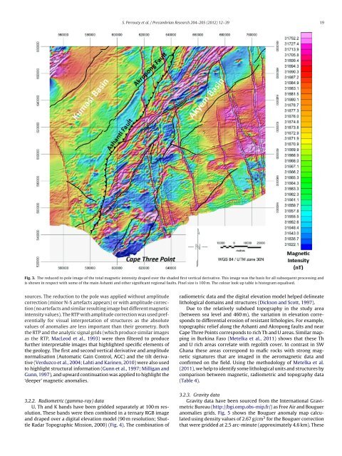
Fig. 3. The reduced to pole image of the total magnetic intensity draped over the shaded first vertical derivative. This image was the basis for all subsequent processing and
is shown in respect with some of the main Ashanti and other significant regional faults. Pixel size is 100 m. The colour look up table is histogram equalised.
sources. The reduction to the pole was applied without amplitude
correction (minor N-S artefacts appears) or with amplitude correction
(no artefacts and similar resulting image but different magnetic
intensity values). The RTP with amplitude correction was used preferentially
for visual interpretation of structures as the absolute
values of anomalies are less important than their geometry. Both
the RTP and the analytic signal grids (which produce similar images
as the RTP, MacLeod et al., 1993) were then filtered to produce
further interpretable images that highlighted specific elements of
the geology. The first and second vertical derivative and amplitude
normalisation (Automatic Gain Control, AGC) and the tilt derivative
(Verduzco et al., 2004; Lahti and Karinen, 2010) were also used
to highlight structural information (Gunn et al., 1997; Milligan and
Gunn, 1997), and upward continuation was applied to highlight the
‘deeper’ magnetic anomalies.
3.2.2. Radiometric (gamma-ray) data
U, Th and K bands have been gridded separately at 100 m resolution.
These bands were then combined in a ternary RGB image
and draped over a digital elevation model (90 m resolution; Shuttle
Radar Topographic Mission, 2000) (Fig. 4). The combination of
radiometric data and the digital elevation model helped delineate
lithological domains and structures (Dickson and Scott, 1997).
Due to the relatively subdued topography in the study area
(between sea level and 460 m), the variation in elevation corresponds
to differential erosion of resistant lithologies. For example,
topographic relief along the Ashanti and Akropong faults and near
Cape Three Points corresponds to rich Th and U areas. Similar mapping
in Burkina Faso (Metelka et al., 2011) shows that these Th
and U rich areas correlate with regolith cover. In contrast in SW
Ghana these areas correspond to mafic rocks with strong magnetic
signatures that are imaged in the aeromagnetic data and
confirmed on the field. Using the methodology of Metelka et al.
(2011), we help to identify some lithological units and structures by
comparison between magnetic, radiometric and topography data
(Table 4).
3.2.3. Gravity data
Gravity data have been sourced from the International Gravimetric
Bureau (http://bgi.omp.obs-mip.fr/) as Free Air and Bouguer
anomalies grids. Fig. 5 shows the Bouguer anomaly map calculated
using density values of 2.67 g/cm 3 for the Bouguer correction
that were gridded at 2.5 arc-minute (approximately 4.6 km). These