Modelling Turbulent Flows with FLUENT - Department of Aerospace ...
Modelling Turbulent Flows with FLUENT - Department of Aerospace ...
Modelling Turbulent Flows with FLUENT - Department of Aerospace ...

Create successful ePaper yourself
Turn your PDF publications into a flip-book with our unique Google optimized e-Paper software.
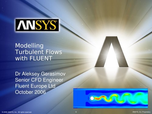
<strong>Modelling</strong><br />
<strong>Turbulent</strong> <strong>Flows</strong><br />
<strong>with</strong> <strong>FLUENT</strong><br />
Dr Aleksey Gerasimov<br />
Senior CFD Engineer<br />
Fluent Europe Ltd<br />
October 2006<br />
© 2006 ANSYS, Inc. All rights reserved. 1 ANSYS, Inc. Proprietary
Is the Flow <strong>Turbulent</strong>?<br />
External <strong>Flows</strong><br />
Re x ≥5 × 10 5<br />
Re D ≥20,000<br />
Internal <strong>Flows</strong><br />
Re ≥ 2 ,300<br />
Dh<br />
along a surface<br />
around an obstacle<br />
where<br />
ρ UL<br />
Re L≡ L = x, D, D h , etc.<br />
Other factors such as freestream<br />
turbulence, surface conditions, and<br />
disturbances may cause earlier<br />
transition to turbulent flow<br />
Natural Convection<br />
Ra≥10 where<br />
8 −10 10 Ra≡ gβΔTL 3 ρ<br />
© 2006 ANSYS, Inc. All rights reserved. 2 ANSYS, Inc. Proprietary<br />
μα
Choices to be Made<br />
Flow<br />
Physics<br />
Accuracy<br />
Required<br />
Turbulence Model<br />
&<br />
NearWall Treatment<br />
Computational<br />
Resources<br />
Turnaround<br />
Time<br />
Constraints<br />
Computational<br />
Grid<br />
© 2006 ANSYS, Inc. All rights reserved. 3 ANSYS, Inc. Proprietary
Turbulence Models in Fluent<br />
ZeroEquation Models<br />
OneEquation Models<br />
SpalartAllmaras<br />
TwoEquation Models<br />
Standard kε<br />
RNG kε<br />
Realizable kε<br />
Standard kω<br />
SST kω<br />
V2F Model<br />
ReynoldsStress Model<br />
Detached Eddy Simulation<br />
LargeEddy Simulation<br />
Direct Numerical Simulation<br />
RANSbased<br />
models<br />
Increase in<br />
Computational<br />
Cost<br />
Per Iteration<br />
Available<br />
in <strong>FLUENT</strong> 6.2<br />
© 2006 ANSYS, Inc. All rights reserved. 4 ANSYS, Inc. Proprietary
RANS Turbulence Models<br />
Spalart<br />
Allmaras<br />
Model Description:<br />
Standard kε<br />
RNG kε<br />
Realizable kε<br />
Standard kω<br />
SST kω<br />
RSM<br />
A single transport equation model solving directly for a modified turbulent viscosity. Designed<br />
specifically for aerospace applications involving wallbounded flows on a fine, nearwall mesh.<br />
Fluent’s implementation allows use <strong>of</strong> coarser meshes. •Option to include strain rate in k<br />
production term improves predictions <strong>of</strong> vortical flows.<br />
The baseline two transport equation model solving for k and ε. This is the default kε model.<br />
Coefficients are empirically derived; valid for fully turbulent flows only. •Options to account for<br />
viscous heating, buoyancy, and compressibility are shared <strong>with</strong> other kε models.<br />
A variant <strong>of</strong> the standard kε model. Equations and coefficients are analytically derived.<br />
Significant changes in the ε equation improves the ability to model highly strained flows.<br />
•Additional options aid in predicting swirling and low Re flows.<br />
A variant <strong>of</strong> the standard kε model. Its ‘realizability’ stems from changes that allow certain<br />
mathematical constraints to be obeyed which ultimately improves the performance <strong>of</strong> this model.<br />
A two transport equation model solving for k and ω, the specific dissipation rate (ε/k) based on<br />
Wilcox (1998). This is the default k ω model. Demonstrates superior performance for wall<br />
bounded and lowRe flows. Shows potential for predicting transition. •Options account for<br />
transitional, free shear, and compressible flows.<br />
A variant <strong>of</strong> the standard kω model. Combines the original Wilcox model (1988) for use near<br />
walls and standard kε model away from walls using a blending function. Also limits turbulent<br />
viscosity to guarantee that τ t ~ k. •The transition and shearing options borrowed from SKO. No<br />
compressibility option.<br />
Reynolds stresses are solved directly <strong>with</strong> transport equations avoiding isotropic viscosity<br />
assumption <strong>of</strong> other models. Use for highly swirling flows. •Quadratic pressurestrain option<br />
improves performance for many basic shear flows.<br />
© 2006 ANSYS, Inc. All rights reserved. 5 ANSYS, Inc. Proprietary
RANS Turbulence Models<br />
Behavior and Usage<br />
Model Behavior and Usage<br />
Spalart<br />
Allmaras<br />
Standard kε<br />
RNG kε<br />
Realizable kε<br />
Standard kω<br />
SST kω<br />
RSM<br />
Economical for large meshes. Performs poorly for 3D flows, free shear flows, flows <strong>with</strong> strong<br />
separation. Suitable for mildly complex (quasi2D) external/internal flows and b.l. flows under<br />
pressure gradient (e.g. airfoils, wings, airplane fuselage, missiles, ship hulls).<br />
Robust. Widely used despite the known limitations <strong>of</strong> the model. Performs poorly for complex<br />
flows involving severe ∇p, separation, strong stream line curvature. Suitable for initial iterations,<br />
initial screening <strong>of</strong> alternative designs, and parametric studies.<br />
Suitable for complex shear flows involving rapid strain, moderate swirl, vortices, and locally<br />
transitional flows (e.g., b.l. separation, massive separation and vortexshedding behind bluff<br />
bodies, stall in wideangle diffusers, room ventilation)<br />
Offers largely the same benefits and has similar applications as RNG.<br />
Possibly more accurate and easier to converge than RNG.<br />
Superior performance for wallbounded b.l., free shear, and low Re flows. Suitable for complex<br />
boundary layer flows under adverse pressure gradient and separation (external aerodynamics and<br />
turbomachinery). Can be used for transitional flows (though tends to predict early transition).<br />
Separation is typically predicted to be excessive and early.<br />
Similar benefits as SKO. Dependency on wall distance makes this less suitable for free shear<br />
flows.<br />
Physically the most sound RANS model. Avoids isotropic eddy viscosity assumption. More CPU<br />
time and memory required. Tougher to converge due to close coupling <strong>of</strong> equations. Suitable for<br />
complex 3D flows <strong>with</strong> strong streamline curvature, strong swirl/rotation (e.g. curved duct,<br />
rotating flow passages, swirl combustors <strong>with</strong> very large inlet swirl, cyclones).<br />
© 2006 ANSYS, Inc. All rights reserved. 6 ANSYS, Inc. Proprietary
Near-Wall <strong>Modelling</strong><br />
Recommended Strategy<br />
• For most high Re industrial applications (Re > 10 6 ) for<br />
which you cannot afford to resolve the viscous<br />
sublayer, use StWF or NEWF<br />
– There is a lot <strong>of</strong> evidence showing that there is little gain from<br />
resolving the viscous sublayer (choice <strong>of</strong> core turbulence model is<br />
more important)<br />
• You may consider using EWT if:<br />
– The same or similar cases ran successfully previously <strong>with</strong> the twolayer<br />
zonal model (in Fluent v5)<br />
– The physics and nearwall mesh <strong>of</strong> the case is such that y + is likely<br />
to vary in a wide range in a significant portion <strong>of</strong> the wall region<br />
– Try to make the mesh either coarse or fine enough, and avoid<br />
putting the walladjacent cells in the buffer layer (y + = 5 ~ 30)<br />
© 2006 ANSYS, Inc. All rights reserved. 7 ANSYS, Inc. Proprietary
Estimating Placement <strong>of</strong><br />
First Near-Wall Grid Point<br />
• Ability for nearwall treatments to accurately predict nearwall flows<br />
depends on placement <strong>of</strong> wall adjacent cell centroids (cell size)<br />
– For StWF and NEWF, centroid should be located in<br />
<br />
loglayer: y p≈30−300<br />
– For best results using EWT, centroid should be located in laminar<br />
<br />
sublayer: y p≈1<br />
• This nearwall treatment can accommodate cells placed in the loglayer<br />
• To determine actual size <strong>of</strong> wall adjacent cells, recall that:<br />
<br />
– y p≡<br />
y pu τ / ν ⇒ y p≡y p ν /uτ<br />
–<br />
u τ ≡ τ w /ρ=U e c f / 2<br />
– The skin friction coefficient can be estimated from empirics:<br />
• Flat Plate c f /2≈ 0 . 037 ReL −0 .2<br />
• Pipe Flow c f /2≈ 0 .039 ReD • Use postprocessing to confirm nearwall mesh resolution<br />
−0. 2<br />
© 2006 ANSYS, Inc. All rights reserved. 8 ANSYS, Inc. Proprietary
Setting Boundary Conditions<br />
• When turbulent flow enters a domain at inlets or outlets (potential<br />
backflow), boundary values for:<br />
– k, ε, ω and/or ui u j must be specified<br />
• Four methods for directly or indirectly specifying turbulence parameters:<br />
– Explicitly input k, ε, ω, or<br />
• This is the only method that allows for pr<strong>of</strong>ile definition.<br />
u i u j<br />
– Turbulence intensity and length scale<br />
• Length scale is related to size <strong>of</strong> large eddies that contain most <strong>of</strong><br />
energy.<br />
– For boundary layer flows: l ≈ 0.4δ 99<br />
– For flows downstream <strong>of</strong> grid: l ≈ opening size<br />
– Turbulence intensity and hydraulic diameter<br />
• Ideally suited for duct and pipe flows<br />
– Turbulence intensity and turbulent viscosity ratio<br />
• For external flows: 1 < μ t /μ < 10<br />
• Turbulence intensity depends on upstream conditions:<br />
u/U≈2k /3 /U 20<br />
© 2006 ANSYS, Inc. All rights reserved. 9 ANSYS, Inc. Proprietary
GUI for Turbulence Models<br />
Define → Models → Viscous...<br />
Inviscid, Laminar, or <strong>Turbulent</strong><br />
Turbulence Model options<br />
Near Wall Treatments<br />
Additional Turbulence options<br />
© 2006 ANSYS, Inc. All rights reserved. 10 ANSYS, Inc. Proprietary
Summary:<br />
Turbulence <strong>Modelling</strong> Guidelines<br />
• Successful turbulence modelling requires engineering judgement <strong>of</strong>:<br />
– Flow physics<br />
– Computer resources available<br />
– Project requirements<br />
• Accuracy<br />
• Turnaround time<br />
– Turbulence models & nearwall treatments that are available<br />
• <strong>Modelling</strong> Procedure<br />
– Calculate characteristic Re and determine if flow is turbulent<br />
– Estimate walladjacent cell centroid y + first before generating mesh<br />
– Begin <strong>with</strong> SKE (standard kε) and change to RNG, RKE, SKO, or SST if<br />
needed<br />
– Use RSM for highly swirling flows<br />
– Use wall functions unless lowRe flow and/or complex nearwall physics<br />
are present<br />
© 2006 ANSYS, Inc. All rights reserved. 11 ANSYS, Inc. Proprietary