Development of the Lake Vegetation Index (LVI) - Edocs

Prepared for:
Assessing the Biological Condition of Florida Lakes:
Development of the Lake Vegetation Index (LVI)
Leska S. Fore
Statistical Design
136 NW 40 th St.
Seattle, WA 98107
leska@seanet.com
Final Report
November, 2005
Russel Frydenborg & Ellen McCarron
Florida Department of Environmental Protection
2600 Blair Stone Rd.
Tallahassee, FL 32399-2400
Aquatic plant found in minimally disturbed lakes. Aquatic plant found in degraded lakes.

ACKNOWLEDGMENTS
Florida Department of Environmental Protection (DEP) biologists provided comments and
guidance throughout the development and testing of the lake vegetation index. R. Frydenborg
provided a description of the study area and unpublished reference material. Data organization
and retrievals, explanation of Florida DEP field and laboratory methods, and general discussions
of plant biology and lake management were provided by J. Espy, T. Frick, R. Frydenborg, E.
McCarron, D. Miller, A. O’Neal, N. Wellendorf, A. Wheeler, and D. Whiting. E. McCarron
provided administrative support and a regulatory perspective. Biologists throughout Florida
collected and identified macrophyte samples, including L. Banks, F. Butera, T. Deck, D. Denson,
J. Espy, K. Espy, T. Frick, R. Frydenborg, S. Gerardi, M. Heyn, J. Jackson, T. Kallemyen, P.
Morgan, P. O’Conner, A. O'Neal, E. Pluchino, D. Ray, J. Richardson, B. Rutter, E. Springer, C.
Swanson, M. Szafraniec, M. Thompson, F. Walton, and A. Wheeler. We thank the Florida DEP
Integrated Water Resource Monitoring program for data used to calculate the human disturbance
gradient. Cover photos courtesy of Wunderlin and Hansen (2004).
ii

TABLE OF CONTENTS
Acknowledgments....................................................................................................................... ii
Table of Contents.......................................................................................................................iii
List of Tables .............................................................................................................................. v
List of Figures............................................................................................................................ vi
List of Appendices ..................................................................................................................... vi
Abstract....................................................................................................................................... 1
Introduction................................................................................................................................. 3
Methods....................................................................................................................................... 5
Study area................................................................................................................................ 5
Lake sampling......................................................................................................................... 6
Quantifying human disturbance.............................................................................................. 8
Metric development and testing............................................................................................ 11
Sensitive and tolerant taxa evaluation................................................................................... 14
Lake Vegetation Index (LVI) development and testing ....................................................... 15
Expectations for statistical correlation.................................................................................. 18
Results....................................................................................................................................... 20
Human disturbance gradient ................................................................................................. 20
Metric selection..................................................................................................................... 21
Sensitive and tolerant taxa .................................................................................................... 31
Evaluation of the Lake Vegetation Index (LVI)................................................................... 33
Correlation of LVI with human disturbance and natural features ................................... 34
Variability analysis of alternative lake sampling protocols ............................................. 35
Metric scoring for the LVI ................................................................................................ 40
Validation of the LVI with independent data .................................................................... 41
Description of outliers ...................................................................................................... 42
Comparison of spring and summer LVI values................................................................. 44
iii

Discussion................................................................................................................................. 46
Human disturbance gradient ................................................................................................. 46
Biological indicators ............................................................................................................. 47
Statistical precision of the Lake Vegetation Index (LVI)..................................................... 48
Recommendations..................................................................................................................... 50
Conclusions............................................................................................................................... 53
References................................................................................................................................. 54
iv

LIST OF TABLES
Table 1. Scoring rules for HDG.....................................................................................................10
Table 2. Examples of LDI coefficient values ................................................................................11
Table 3. Coefficient of conservatism (CC) scoring criteria ..........................................................13
Table 4. Correlation for HDG and its component measures..........................................................20
Table 5. Comparison of water chemistry measures for porous and non-porous soils ...................21
Table 6. Candidate plant metrics and their correlation with HDG, WQ index, LDI, and habitat
index...............................................................................................................................................23
Table 7. Plant taxa most frequently identified as dominant...........................................................25
Table 8. Plant taxa that were significantly associated with low or high HDG ..............................32
Table 9. Correlation between LVI, measures of disturbance, and natural features.......................34
Table 10. Coefficients from multiple regression for LVI and its component metrics...................35
Table 11. Cumulative number of taxa for 12 lake sections ...........................................................36
Table 12. Variance estimates and number of detectable categories for LVI .................................37
Table 13. Correlation between LVI, its component metrics and HDG for different sampling
methods..........................................................................................................................................39
Table 14. Correlation between LVI and measures of disturbance for different numbers of
replicate LVI samples ....................................................................................................................40
Table 15. Metric scoring rules for LVI..........................................................................................41
Table 16. Correlation between LVI and measures of disturbance for the validation data set .......42
Table 17. Lakes with higher or lower LVI values than predicted by HDG...................................43
v

LIST OF FIGURES
Figure 1. Diagram showing 12 lake sampling sections ...................................................................7
Figure 2. Detail of lake section sampling methods..........................................................................8
Figure 3. LVI plant metrics plotted against HDG..........................................................................27
Figure 4. LVI plant metrics plotted against the WQ index............................................................28
Figure 5. LVI plant metrics plotted against the habitat index........................................................29
Figure 6. LVI plant metrics plotted against LDI............................................................................30
Figure 7. Plant CC value plotted against the average HDG for lakes in which taxon was found .33
Figure 8. Species accumulation curve for lake sections ................................................................36
Figure 9. Number of categories that LVI could detect for different sampling protocols ..............38
Figure 10. Distribution of LVI values............................................................................................39
Figure 11. LVI plotted against HDG for the validation data set....................................................42
Figure 12. LVI plotted against HDG with outliers indicated.........................................................43
Figure 13. LVI for repeat visits during spring and summer for 15 lake sites................................45
Figure 14. Diagram showing recommended lake sampling for LVI .............................................50
Appendix 1. Aquatic plant attributes
Appendix 2. EPA’s wetland plant attributes
LIST OF APPENDICES
Appendix 3. Results of testing for tolerance and sensitivity
Appendix 4. LVI values by district
Appendix 5. Additional tables
vi

ABSTRACT
The Florida Department of Environmental Protection (DEP) is required under the regulations of
the Clean Water Act to assess the biological condition of its streams, rivers and lakes. We
developed a multimetric index, the Lake Vegetation Index (LVI), to assess the biological
condition of aquatic plant communities in Florida lakes. For the development and testing of the
LVI, aquatic plants in 95 lakes were sampled by boat during 2000–03. To validate the results for
the LVI, data from an additional 63 lakes were collected in 2004; these data included 15 lakes
with repeat visits for spring and summer. A total of 48 candidate metrics based on measures of
community structure, taxa richness, and percent of total taxa were calculated and tested against
independent measures of human disturbance. An additional 17 metrics derived from plant
information from a national database were also evaluated. To test metrics, we developed a
human disturbance gradient (HDG) that summarized measures of water chemistry, habitat
condition, intensity of land use in a 100 m buffer around the lake, and hydrologic modifications.
A total of 10 metrics met the targeted values for correlation with HDG; of these ten, four were
not redundant with each other and were included in the LVI: percent native taxa, percent
invasive taxa, percent sensitive taxa, and the average tolerance value of the taxon present over
the largest area (dominant C of C).
Tolerant and sensitive taxa were defined based on designations made by 10 expert
botanists working independently to define coefficient of conservatism (CC) scores for wetland
(not lake) plants in Florida. Metrics derived from CC scores were highly correlated with HDG.
In contrast, relatively few individual taxa were significantly associated with HDG: only 29 out of
404 taxa showed significant preferences. Rare taxa were partially to blame for weak results, over
half the 404 taxa were found in < 5 lakes.
Plant data were collected from each of 12 lake sections, and taxa lists from the 12
sections were kept separate. Using the replicate data, we compared the ability of different
sampling protocols to detect differences in lake condition. Based on LVI calculated and averaged
from four lake sections, LVI could detect five categories of biological condition.
1

LVI was highly correlated with HDG and other independent measures of human
disturbance for both the development and the validation data sets (-0.68 and -0.72, Spearman’s
r). For the 15 lakes with repeat visits, LVI values for repeat visits within the year were more
variable than for repeat visits on the same-day; however, neither spring nor summer LVI values
were consistently higher across lakes. We conclude that LVI is a reliable indicator of lake
condition and has sufficient statistical precision to detect multiple levels of biological condition.
Given the relatively small data sets available for this study (

INTRODUCTION
A primary objective of the federal Clean Water Act (CWA) is “to restore and maintain the
chemical, physical, and biological integrity of the Nation’s waters.” Under the CWA, each state
must develop water quality standards for all its surface waters. Water quality standards include
designated uses assigned to a water body, water quality criteria to protect the uses, and an
antidegradation policy (Ransel, 1995; Karr et al., 2000). Until the late 1980s, most states used
primarily chemical criteria to assess surface waters. A shift occurred when resource managers
realized that chemical criteria alone often fail to protect aquatic life uses (Karr and Chu, 1999).
At that time, EPA mandated that states adopt biological criteria for the protection of water
resources (Karr, 1991).
The state of Florida recognizes the importance of biological monitoring of water
resources and has developed sampling protocols to assess the condition of streams, lakes, and
wetlands based on their biological assemblages (Barbour et al., 1996; Gerritsen and White, 1997;
McCarron and Frydenborg, 1997; Fore, 2004; Lane et al., 2004; Reiss and Brown, 2005). Florida
Department of Environmental Protection (DEP) uses bioassessments derived from these
protocols to define acceptable conditions for the support of aquatic life uses. Within the context
of the CWA, bioassessments can be used to define impairment, evaluate best management
practices, develop targets for management plans or restoration, or identify exceptional resources
for protection (Yoder and Rankin, 1998; Karr and Yoder, 2004).
Compared to rivers, streams, and wetlands, relatively less work has been done to develop
biological monitoring tools for lakes (USEPA, 2002a, 2002b; but see Whittier et al., 2002 and
Harig and Bain, 1998 for lake indicator development). While most states have biological
assessment programs in place for rivers and streams, Florida is one of only nine states with lake
or reservoir bioassessment programs in place and one of only three that is developing numeric
biocriteria for lakes (Gerritsen and White, 1997; USEPA, 2003). In many states, lakes may
represent a smaller proportion of surface waters; however, with more than 7700 lakes greater
than 10 acres in size, lakes represent a significant natural resource in Florida.
3

Although lakes are not wetlands, they share many of the same habitats and taxa within a
particular region. The U.S. Environmental Protection Agency (EPA) has recently supported
numerous research efforts related to the development of bioassessment and biocriteria for
wetlands (USEPA, 2002b). Resources developed for wetland assessment were borrowed and
applied for this study of lakes. For example, extensive literature surveys have documented the
current science for wetland monitoring at the national level (Adamus et al., 2001) and
specifically for Florida (Doherty et al., 2000). Documents published by EPA summarize the
aquatic plant metrics that have been successfully applied in wetlands throughout the U.S. and
this information was very helpful in identifying potential metrics for this study (USEPA, 2002c).
Similar lists of candidate metrics for aquatic plants in lakes have not been developed (Gerritsen
et al., 1998). Another source for potential metrics was Ohio EPA which has tested several types
of plant metrics for inclusion in their vegetation IBIs for wetlands (Mack, 2004). Within Florida,
the multimetric indices developed for isolated depressional herbaceous wetlands by Lane et al.
(2004) and for isolated depressional forested wetlands by Reiss and Brown (2005) included
additional metrics that were tested in this study for lakes. Finally, a study by Cohen et al. (2004)
used the professional experience of 10 botanists to define aquatic plant tolerance and sensitivity
to disturbance in wetlands. We used these designations to define sensitive and tolerant plant taxa.
The purpose of this study was to develop a monitoring and assessment tool for lakes
based on aquatic plant sampling. Though used extensively in wetland monitoring, aquatic plants
are rarely selected as indicators of lake condition (but see Nichols et al., 2000 for a Wisconsin
index). Aquatic plants provide an effective endpoint for monitoring lake condition for several
reasons: 1) a wide array of plants with a variety of life history strategies are represented in
Florida lakes, 2) much is known about the specific preferences and tolerances of many these
plants, and 3) collecting and identifying plants in the field is relatively straightforward which
means that laboratory costs are minimal. The goals of this study were to identify potential
metrics for aquatic plants, test them against an independent gradient of human disturbance,
combine the metrics into a lake vegetation index (LVI), and determine the most efficient method
for collecting plant data to calculate the index.
4

METHODS
Study area
The state of Florida can be divided into three geographic regions based on watershed drainage
patterns: the northern panhandle, the southern peninsula, and a transition region known as the
northeast. These three regions were used to develop and test a multimetric index for invertebrates
because different species assemblages were associated with these three geographic areas
(Barbour et al., 1996; Fore, 2004). Sufficient data did not exist for lake plants to perform a
similar test for associations between geographic areas and plant species assemblages;
consequently, we used the geographic areas derived from watershed drainage patterns to test for
regional differences in metric values.
The middle and lower Suwannee basin provides a natural demarcation between the
panhandle and peninsula, with the northeast region straddling the upper Suwannee northeast of
the Cody escarpment (White, 1970). Terrestrial vegetation communities in the panhandle
generally consist of mixed pine/oak/hickory forests (Pinus spp., Quercus spp., Carya spp.),
longleaf pine forests (Pinus palustris), hardwood forests with beech/magnolia climax community
(Fagus grandiflora/Magnolia grandiflora), and swamp hardwood forests of cypress (Taxodium
spp.) or tupelo (Nyssa spp.), interspersed by a mosaic of pine plantations, cropland (e.g., corn,
soy beans, peanuts), and pasture (SWCS, 1989; Fernald and Purdum, 1992). The panhandle is
less densely populated by humans than the other areas.
The peninsula has a sandy highland ridge extending down its center almost to Lake
Okeechobee. The elevation of the central ridge is approximately 150 to 200 ft. Terrestrial
vegetation communities on the ridge of the peninsula consist of longleaf pine/turkey oak forests
(Pinus palustris/Quercus laevis), on flat areas are slash pine (Pinus eliottii) or loblolly pine
(Pinus teada) with palmetto/gallberry understory (Serenoa repens/Ilex glabra), and in
depressional areas are marsh/wet prairies (maidencane, pickerel weed), and hardwood wetlands
of sweetbay (Magnolia virginiana), cypress (Taxodium spp.), and ash (Fraxinus spp.; SWCS,
1989). The dominant land use is pasture, cropland (e.g., watermelons, nursery products,
5

tomatoes), and urban areas (Fernald and Purdum, 1992). Dense population centers are located at
Tampa and Orlando.
The northeast region includes portions of the Okeefenokee Swamp, parts of the upper
Suwannee drainage, the Black Creek drainage, and the Sea Island flatwoods. Plant communities
consist of longleaf pine/turkey oak (Pinus palustris/Quercus laevi) on the sandy uplands,
hardwood wetlands of cypress (Taxodium spp.), tupelo (Nyssa spp.), and loblolly bay (Gordonia
lasianthus), pine flatwoods, and marsh (FNAI, 1990). Jacksonville is the only major population
center.
Lake sampling
For this study, lakes were defined as fresh water bodies with >= 2 acres of open water of
sufficient depth and size to require a boat for sampling. Two different data sets were used to
develop and validate the LVI. The first data set included 95 lakes that were selected to represent
a broad range of site conditions and human influence across the state. These lakes were used to
test metrics and develop the LVI. Lakes were sampled by Florida DEP during August–
November, 2000–2003. Of the 95 lakes, 17 were located in the panhandle region, 74 in the
peninsula, and 4 in the northeast. Lake surface area was known for 80 lakes and ranged from 8–
3500 acres with a mean of 343 acres. Lakes were not selected randomly, nor were they selected
to ensure coverage in all ecoregions. Consequently some geographic areas were not included.
The second data set included 63 additional lakes, and these data were used to validate the
correlation between LVI and independent measures of human disturbance. These lakes were
sampled during March–September, 2004; 34 lakes were located in the panhandle and 29 in the
peninsula. Of these lakes, 15 small lakes from the panhandle were sampled during spring and
summer and were used to test for seasonal differences in LVI.
Aquatic macrophytes include aquatic plants large enough to be easily seen by the unaided
eye, as well as some larger algae such as Nitella and Chara. Aquatic macrophytes grow in water
or wet areas and may be rooted in the sediment or floating on the water’s surface. Most aquatic
macrophytes are vascular plants and include herbaceous species as well as trees and shrubs.
6

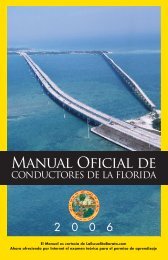
Each lake was sampled 12 times by dividing the lake into 12 approximately wedgeshaped
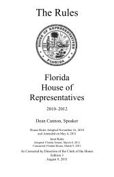
sections, depending on the shape of the lake (Figure 1). Within each section, two methods
were used to identify plants: 1) from the boat, plants were identified, using either binoculars or
the unaided eye, while boating slowly along the shore, and 2) plants were also identified within a
5 m belt transect. The transect was perpendicular to the shore, from the mean high water mark
towards the center of the lake. For the belt transect, visible plants were identified and submersed
plants were also sampled with a standard frotus, a device which enables the collection of
underwater plants. The frotus was deployed 5 times along each 5 m belt transect (Figure 2).
Lakes sampled before the fall of 2003 used only the drive-by method (35 of the 95 lakes in the
development data set), while lakes sampled during or after fall 2003 used both methods. Plants
identified using the two above methods were combined into a single taxa list, one for each of the
12 sections.
The plant judged to have the greatest areal extent, determined visually, within each of the
12 lake sections was denoted as “dominant,” while all others were recorded as “present.” If two
taxa were more abundant than the other plants present, they were noted as “co-dominant.” If the
degree of dominance was not readily determined, all plants in the sampling unit would simply be
marked “present.” Plants were identified to the lowest taxonomic level possible, typically
species. Unknown species were placed on ice and sent to an expert for identification.
9
10
8
11 12 1 2
7
6
Figure 1. Diagram showing the method used to divide a typical lake into
12 sections for replicate sampling.
5
3
4
7

Frodus deployment
Drive-by
Submersed Zone
Emergent Zone
5 m Belt Transect
Figure 2. Detail of sampling methods used to identify plant taxa
within a lake section.
Quantifying human disturbance
Karr and colleagues describe five factors to summarize the ways in which humans alter and
degrade rivers and streams (Karr et al., 1986; Karr et al., 2000). The five factors are flow regime,
physical habitat structure, water quality, energy source, and biological interactions. For this study
data were available to evaluate three of these factors (water quality, physical habitat structure,
and flow regime), as well as human disturbance at the watershed scale.
To evaluate lake water chemistry, Florida DEP biologists measured conductivity, total
Kjeldahl nitrogen (TKN), nitrites/nitrates (NOx), total phosphorus (TP), and algal growth
potential (AGP). We summarized information from these five measures into a water quality
(WQ) index by converting values for each measure into unit-less scores and then averaging the
scores. To convert to unit-less scores, we used the percentiles from a statewide data set
(Integrated Water Resource Monitoring [IWRM] Cycle 1, 2000-2003) to define expectations.
For the IWRM Cycle 1 study, water chemistry data were collected from ~1100 randomly chosen
8

lakes. If the observed value from the LVI index development data set was < 10 th percentile value
observed for the statewide IWRM data set, the lake-visit received a score of 1 for that chemistry
measure; if < 20 th percentile the lake-visit scored a 2; and so on. We repeated this process for
each of the five chemical measures. After scoring each of the measures, we averaged the unitless
scores (ignoring missing data) for all the chemical measures to define the water quality
(WQ) index. For the 95 lakes in the index development data set, 10–25 had missing values for
one or more of the chemical measures. To test whether missing values contributed to the
correlation (or lack of correlation) between the WQ index and other measures of disturbance,
correlation was also tested for sites without missing data.
For each lake, DEP biologists also evaluate habitat condition by assigning numeric scores
to qualitative descriptions of vegetation quality, stormwater inputs, bottom substrate, lakeside
human alterations, upland buffer zone, and watershed land use (DEP protocol FT-3200). These
scores are summed to yield a single value, the habitat index. Sufficient information was not
available to develop a similar index for hydrologic condition. Instead, each lake was assigned a
score of 0 if no hydrologic modification was observed or 1 if the lake was impounded or its
hydrology artificially controlled.
Human land use around each lake was derived from aerial photos of 1995 land use
coverages and a 100 m buffer area around the lake defined. Land use within the buffer was
summarized using an index developed to estimate the intensity of human land use based on
nonrenewable energy flow (Brown and Vivas, 2004). The landscape development intensity
(LDI) index was calculated as the percentage area within the catchment of a particular type of
land use multiplied by the coefficient of energy use associated with that land use, summed over
all land use types found in the catchment (Table 1).
∑(
LDIi
LU )
LDI %
Where,
= i
* .
LDIi = the nonrenewable energy land use for land use i, and
%LUi = the percentage of land area in the catchment with land use i.
To define the human disturbance gradient (HDG), we converted the four measures of
human disturbance (the water quality index, the habitat index, the measure of hydrologic
9

condition, and the LDI) to unit-less scores and summed the scores to define HDG values for each
lake-visit. Three of the measures had scores of 0, 1, or 2 indicating low, moderate or high levels
of human influence. One measure, hydrologic condition, only had scores of 0 or 1 (Table 2).
HDG ranged from the minimum value of 0 to the maximum of 7 for the 95 lakes in the
development data set. Each of the eight categories of HDG was represented by 6–18 lakes with
the extreme values (HDG = 0, 6, or 7) having the fewest lakes.
Table 1. Description of land use and the coefficient value used to calculate the LDI. Higher
values indicate greater intensity of human land use.
Land use LDI value
Natural Open water 1.00
Pine Plantation 1.58
Woodland Pasture 2.02
Pasture 2.77
Recreational / Open Space (Low-intensity) 2.77
Low Intensity Pasture (with livestock) 3.41
Citrus 3.68
High Intensity Pasture (with livestock) 3.74
Row crops 4.54
Single Family Residential (Low-density) 6.79
Recreational / Open Space (High-intensity) 6.92
High Intensity Agriculture 7.00
Single Family Residential (Med-density) 7.47
Single Family Residential (High-density) 7.55
Low Intensity Highway 7.81
Low Intensity Commercial 8.00
Institutional 8.07
High Intensity Highway 8.28
Industrial 8.32
Low Intensity Multi-family residential 8.66
High intensity commercial 9.18
High Intensity Multi-family residential 9.19
Low Intensity Central Business District 9.42
High Intensity Central Business District 10.00
10

Table 2. Scoring rules for measures used to calculate the human disturbance gradient (HDG).
HDG is the sum of the scores.
Measure 0 1 2
WQ index =6
Habitat index >65 45–65

each expert were averaged to derive a single CC score for each taxon. The CC scores were
developed for depressional marshes in Florida, not for lakes (Cohen et al., 2004).
Community structure – The total number of taxa found is expected to decline as human
disturbance eliminates habitat, changes water chemistry, and interrupts the natural hydroperiod.
Although some studies have documented a decline in the number of wetland taxa as disturbance
increases (Findlay and Houlahan,1997; Lopez et al., 2002), this metric is not typically chosen for
wetland monitoring (USEPA, 2002c). The number of plant guilds summarized the number of
different types of plants present at a lake, e.g., forb/herb, graminoid, shrub, tree, or vine. The
number of plant guilds is expected to decline with disturbance. We expect more tolerant plants to
dominate the assemblage as disturbance increases. Dominant C of C was defined as the CC score
for the one or two plants that covered the greatest area.
Nativity – Native taxa are those whose natural range included Florida at the time of European
contact (1500 AD). Exotic taxa are species introduced to Florida from a natural range outside of
Florida. Definitions of invasive taxa were taken from lists developed by the Florida Exotic Pest
Plant Council. FLEPPC defines Category I invasives as “exotics that are altering native plant
communities by displacing native species, changing community structures or ecological
functions, or hybridizing with natives” (FLEPPC, 2003). Category II invasives are defined as
“exotics that have increased in abundance or frequency but have not yet altered Florida plant
communities to the extent shown by Category I species.” For 95 lakes in the development data
set, 17 taxa were listed as Category I and 7 as Category II. (See Appendix 1 for plant attributes.)
Threatened and endangered species – Four endangered species (Xyris isoetifolia, Hypericum
lissophloeus, Salix eriocephala, and S. floridana) and one threatened species were found
(Drosera intermedia). Five species did not provide enough range of values to define a metric and
no metric was tested for this attribute.
Tolerance/Sensitivity – Coefficient of conservatism (CC) scores were available for 240 of the
404 taxa found. CC scores are most typically used to calculate a ‘floristic quality index (FQI)’
(Lopez and Fennessy, 2002). FQI was calculated as the average CC value multiplied by the
square root of the total number of plant taxa. The simple mean of the CC scores has also been
reported and was tested here. Lane et al. (2004) found that mean CC score was significantly
12

correlated with LDI for herbaceous wetlands in Florida. We calculated the total number of
sensitive and tolerant taxa by defining taxa with a CC score > 7 to be sensitive and CC < 3 to be
tolerant (Table 3). Percent sensitive and tolerant taxa were selected as metrics for both the
herbaceous and forested wetland indices in Florida (Lane et al., 2004; Reiss and Brown, 2005).
Duration – Lakes with less human disturbance are expected to have a greater number of
perennial taxa or a higher relative proportion of perennial taxa than annual taxa. Annual taxa
represent more opportunistic taxa which tend to be associated with human disturbance. Ohio
EPA uses the ratio of annual to perennial taxa in several of its vegetation indices for wetlands
(Mack, 2004).
Table 3. Coefficient of conservatism (CC) scoring criteria (after Cohen et at., 2004; Andreas
1995) and designations used to define a plant as tolerant or sensitive for this study.
CC
score
Sensitive or
Tolerant
Criteria
0 T Alien taxa and native taxa that are opportunistic invaders
1–3 T Widespread taxa that are found in a variety of communities,
including disturbed sites
4–6 Neither Taxa that display fidelity to a particular community, but tolerate
moderate disturbance
7–8 S Taxa that are typical of well-established communities, which have
sustained only minor disturbances
9–10 S Taxa that exhibit high degrees of fidelity to a narrow set of
ecological conditions
Wetland status – Although all sampling locations were defined as lakes and not wetlands, we
tested metrics related to wetland status because extensive lists have been developed for many
plants and because wetland status may provide an indicator of hydrologic alteration or other
types of human disturbance in lakes (USEPA, 2002c). Species defined as ‘obligate wetland’ or
‘facultative wetland’ plants are considered to be adapted to life in anaerobic soils (USACE,
1987); facultative species are equally likely to occur in wetlands or non-wetlands; and upland
species are expected not to occur in wetlands.
13

Growth form – This category included several aspects of plant growth. Metrics were calculated
for herbaceous and woody taxa and for emergent, floating, and submersed taxa. Fern and
gymnosperm taxa were also summarized. The previous metrics were also calculated for native
taxa only. In addition, candidate metrics based on native forbs+herbs, graminoids, nonvascular
plants, vines, shrubs, subshrubs and trees were tested. Nichols et al. (2000) suggest that the
relative frequency of submersed taxa may be greater than floating or emergent taxa when water
quality is degraded. Emergent species may also tolerate greater wave action. Other studies
suggest that emergent species may increase with an increase in nutrients while submersed taxa
decline (Doherty et al., 2000).
Dicot/monocot – Flowering plants (angiosperms) are divided into two groups depending on the
number of cotyledons found in the embryo. The cotyledons are the seed leaves produced by the
embryo. In Ohio, native dicots decline with increasing disturbance and this metric is included in
four out of five Ohio wetland indices (Mack, 2004).
Additional metrics derived from the national wetland database – In addition, several metrics
were derived from a national database of plant characteristics developed for wetland plants
(Adamus and Gonyaw, 2000). Information in this database was derived from published, peerreviewed
studies. Development of this database was funded by EPA in response to requests from
state agencies involved in monitoring wetlands. The attributes were derived from literature
surveys for each taxon and summarized information regarding general sensitivity or tolerance,
tolerance to nutrients, nitrogen or phosphorus, and sensitivity or tolerance to flooding, sediment,
and salinity (Appendix 2). Of the 404 taxa found in the 95 lakes, 137 were listed in the EPA
database.
Sensitive and tolerant taxa evaluation
We tested the association of individual plant taxa with the HDG using a 2 x 2 contingency table
analysis (χ 2 , Yates correction, α = 0.05). Lakes with an HDG of 0, 1, or 2 were defined as ‘good’
lakes (N = 36), and the remaining 59 lakes with HDG from 3–7 as the ‘poor’ lakes. An HDG < 3
meant that a lake could have moderate disturbance indicated for two measures or high
disturbance for a single indicator. This statistical approach tests whether occurrence of an
individual plant taxon depended on the level of human disturbance.
14

We also calculated the average HDG value for all the lakes at which a particular taxon
was found and compared this empirical value for sensitivity (or tolerance) to the CC values
derived from expert judgment. This approach was not intended as a potential metric, but as a test
of the CC scores for the lakes data set.
Lake Vegetation Index (LVI) development and testing
Candidate metrics were considered for inclusion in the LVI if they were significantly correlated
with the HDG (Spearman’s r >= 0.4 or

versions were so similar. Furthermore, we were interested in the smallest amount of sampling in
order to minimize field effort.
For all three versions of the LVI, the index was calculated by first transforming metrics
into unit-less scores on the basis of their 5 th and 95 th percentiles. Leaving out the upper and lower
5% of metric values eliminates extremely high or low values that may not be typical of
minimally or extremely disturbed sites. The 95 th percentile value was assigned a score of 10 (for
metrics that declined with disturbance such as percent native taxa) and the 5 th percentile value
was assigned a score of 0. For metrics that increased with disturbance the scores were reversed
for the 5 th and 95 th percentiles. After transformation, metric scores ranged from 0–10. The LVI
was the sum of the four metrics multiplied by a constant to adjust the range of LVI to a 0–100
scale. A scale from 0–100 was selected for convenience with the intention of keeping the same
scale for all Florida multimetric indices (Hughes et al., 1998).
We used non-parametric correlation to test association between LVI_12x and lake
surface area, latitude, and longitude. Because LVI_12X was significantly correlated with latitude
as well as HDG, we used multiple regression to evaluate the relationship between LVI_12x and
these independent variables. After confirming that human disturbance was the primary correlate
for both LVI_12x and its component metrics, we next addressed the question of how many lake
sections should be sampled. We evaluated the different versions of the index using two criteria:
1) LVI correlation with human disturbance and 2) the number of categories of biological
condition that each version of the index could detect.
We estimated within-lake variability of the different versions of LVI using an ANOVA
model. We used lake as the main factor and repeat samples within each lake were defined as
replicates and used to calculate the mean squared error (MSE). This estimate of variance was
used to calculate a 90% confidence interval for different versions of LVI (Zar, 1984). The
confidence interval was calculated as:
16

LVI
⎛ 2 ⎞
⎜ s
± * 1.
645⎟
⎜ ⎟
⎝
n
⎠
,
where s 2 = variance estimated from ANOVA (mean squared error), and
n = number of samples taken from the lake.
The number of categories of biological condition that LVI can reliably detect was
obtained by dividing the possible range of the index (0–100) by the confidence interval. Thus,
the confidence interval defined the level of precision of the index by representing how different
LVI would have to be during a subsequent lake-visit to conclude that a statistically significant
change had occurred in lake condition. That confidence interval was also used to define how
many non-overlapping categories of biological condition could be defined over the potential
range of LVI. To compare the different versions of LVI, we looked at the number of categories
of biological condition each version could reliably detect for different numbers of replicate
samples.
We used z-values from the normal distribution to calculate 90% confidence limits for
LVI for two reasons. First, the distribution of multimetric indices are known to approximate the
normal distribution in that they are unimodal and symmetric (Fore et al., 1994). Second, for
small sample sizes, the t-distribution is appropriate for calculating confidence limits because
variance may be underestimated; however, for large sample sizes (df > 30) the two distributions
converge. For this data set, data from 95 lakes provided an adequate sample size to apply the
normal distribution. An additional concern when estimating variance is that the full range of
expected values are represented. LVI values for this data set ranged from 0–100, which included
all possible values for the index.
To validate the results based on the development data set of 95 lakes, an additional 63
lakes were sampled in 2004. LVI, HDG, the WQ index, the habitat index and LDI were
calculated for these additional lakes and tested for correlation. Fifteen of these lakes were
sampled twice during 2004, once during spring (March–April) and again during the summer
(July–August).
17

Expectations for statistical correlation
The statistical significance of a correlation coefficient (r) is a function of the sample size, such
that for larger sample sizes a smaller correlation coefficient will be significant. For large data
sets, e.g., N = 100, a correlation coefficient of 0.17 will be statistically significant (alpha = 0.05,
1-sided test). Such a small correlation coefficient may be statistically significant but biologically
not very meaningful. Consequently, before correlation testing is complete, a scientist should
consider the underlying meaning of correlation coefficients and what values represent biological
significance.
Based on these considerations, we selected specific values for correlation coefficients that
would represent a meaningful association depending on which relationship was being tested. We
used a correlation coefficient for metrics > 0.4 to define a significant relationship with HDG,
then further evaluated each metric by looking at scatter plots. Thus, for metric selection, a higher
standard was set than simple statistical significance. For metric correlation with the HDG, we
anticipated that the variability associated with HDG and the inherent difficulty involved in fully
assessing human influence would mean that high correlation coefficients (e.g., > 0.7) would be
unlikely. On the other hand, correlation coefficients < 0.4, though they may be statistically
significant, tend to be unconvincing when graphed.
Using graphs, we tested to be sure that the lack of correlation was not due to good metric
values in sites where human disturbance was known to be high. In contrast, we tolerated poor
metric values in sites with no known disturbance because the HDG does not include many
potential sources of degradation (e.g., herbicides).
To test for metric redundancy, we first screened metrics to determine whether a metric
pair’s correlation was greater than 0.8. We expected metrics to be highly correlated with each
other because they were initially selected for their correlation with the same underlying measure,
the HDG. When selecting metrics for the LVI, we wanted to be sure that the metrics were not
redundant in that they were derived from the same information (species). If a metric pair was
highly correlated, we evaluated the metrics to determine whether the same taxa were used in
calculation of both metrics. When metrics were derived from redundant information, one metric
18

in each pair (or group) was selected on the basis of its correlation with HDG, biological meaning,
and sensitivity to degradation.
When testing for correlation between biological measures (LVI and its component
metrics) and physical measures (lake surface area, latitude, and longitude) we were less tolerant
of correlation. For this analysis, any statistical significant correlation was considered because we
were concerned that underlying natural features or processes could bias the biological assessment
of LVI. We wanted to be sure that smaller lakes, for example, did not consistently score lower
for LVI for the same level of human disturbance. Thus, in different testing situations, different
values for the correlation coefficient were selected to indicate a significant association before
testing.
19

RESULTS
A total of 404 taxa were identified from the 95 lakes in the index development data set. Most
plants were identified to species, in some cases plants were identified to genus (e.g., Bidens,
Cyperus, Ludwigia, Panicum, Xyris), and in a very few cases to family. The number of taxa
identified in a lake based on the combination of data from all 12 sections ranged from 13–57,
with an average of 34 taxa. The number of taxa found in a single lake section (1 of 12) ranged
from 1–44 with an average of 15 taxa (Kell-Air and Karick Lakes had the lowest value of one
taxon in a section and Lake Juliana had 44 taxa in one section).
Human disturbance gradient
The HDG was highly correlated with its component measures, indicating that HDG effectively
integrated site condition for all three component measures (Table 4). Overall, each individual
measure of human disturbance was more highly correlated with the HDG than with other
measures, suggesting that the HDG was a better measure of general human disturbance.
Hydrologic condition was not tested for correlation because it had only two possible values. The
WQ and habitat indices were also highly correlated with each other, as were the habitat index
and the LDI. In contrast, the WQ index was not significantly correlated with LDI, indicating that
land use was not a good predictor of water quality condition for this data set. When only sites
with no missing values for water quality variables were tested for correlation, values for the
correlation coefficient changed little (< 0.04).
Table 4. Correlation for measures of human disturbance and the HDG, only significant
correlations are shown (Spearman’s r, p < 0.01). Index values were tested for correlation using
their original values, not the scores (0, 1, 2) used to calculate the HDG.
HDG WQ index Habitat index LDI
HDG 0.62 -0.87 0.73
WQ index 0.62 -0.46
Habitat index -0.87 -0.46 -0.69
LDI 0.73 -0.69
20

Because the WQ index and LDI were not highly correlated, we tested whether soil type
could explain the lack of correlation (Florida GIS coverage STATSGO soils). Some soils are
more porous than others and for lakes in porous soils, chemicals or pollutants may run into the
soil rather than run off the surface and into the lake. Lakes surrounded by non-porous soils may
have higher levels of chemicals. We used a nonparametric two-sample test to check for
differences in the WQ index, conductivity, NH3, TKN, NOx, TP, orthophosphates (OP), chloride,
and sulfate. Conductivity, TP, and TKN were significantly higher in lakes with non-porous soils
(Mann-Whitney U test, 1-sided, p < 0.05; Table 5). NOx was significant, but not in the direction
predicted, values were lower in lakes with non-porous soil. Though statistically significant, the
differences between levels of chemical measures in porous and non-porous soils were probably
not large enough to explain the lack of correlation between the WQ index and LDI.
Table 5. Water quality measure, and statistics from Mann-Whitney U test including rank sums
for non-porous (NP) and porous (P) soils, U-statistic, z-statistic, sample size (N), and p-value.
Significantly different measures are marked with an *.
WQ measure Rank Sum NP Rank Sum P U Z N (NP) N (P) p
WQ index 1901.0 2285.0 959.0 0.49 40 51 0.31
* Conductivity 2070.5 2024.5 749.5 2.03 40 50 0.02
* TKN 1662.0 1824.0 648.0 1.77 35 48 0.04
NOX 1294.0 2361.0 591.0 -2.63 37 48 0.00
* TP 1972.5 1855.5 630.5 2.57 38 49 0.01
AGP 1273.5 1576.5 678.5 -0.20 34 41 0.42
OP 564.0 517.0 264.0 0.00 24 22 0.50
NH3_N 1624.5 2203.5 883.5 -0.41 38 49 0.34
Chloride 371.0 532.0 181.0 0.70 16 26 0.24
Sulfate 390.0 513.0 162.0 1.19 16 26 0.12
Metric selection
Many candidate metrics were tested and relatively few were strongly correlated with HDG or
consistently correlated with the other measures of human disturbance. Of the 65 metrics tested
for correlation with HDG, only 10 had an r-value > 0.4 (or < –0.4; Table 6). Because many of
these metrics were redundant, a total of four metrics were selected for the final multimetric
21

index. In general, if a candidate metric was correlated with HDG when calculated as number of
taxa, it was also correlated with HDG when calculated as percentage of total taxa. In addition, if
a candidate metric was correlated with HDG, it was typically correlated with at least two of the
other measures of disturbance.
Overall, the metrics that measured the numbers of native and exotic taxa and metrics
derived from CC values were the most consistently associated with human disturbance. Within
specific metric categories, results for individual metrics tended to be similar. Of the three metrics
related to community structure, only dominant C of C was significantly correlated with HDG and
was included in the index. A total of 63 taxa were identified as dominant in at least one lake
section. Of these 63 taxa, about 1/3 were identified only once and about 1/3 were identified >10
times as dominant (Table 7). Total number of taxa and the total number of growth forms were
not correlated with HDG.
Of the four metrics related to nativity, all were significantly correlated with HDG, but the
three based on exotic taxa were redundant. Category I and II invasives represented a subset of
the exotic taxa. We retained percent invasive taxa for the LVI because invasive taxa represent a
significant economic concern and an objective threat to native plant assemblages. We calculated
this metric as a percentage of total taxa rather than total number of taxa because this form of the
metric was less affected by geographic factors such as latitude. We also included percent native
taxa in the index which was only significantly associated with HDG when calculated as a
percentage of total taxa.
22

Table 6. Candidate plant metrics and their correlation with HDG, the WQ index, LDI, and the
habitat index. Only Spearman’s correlations >0.40 are shown ( p < 0.001). The sample size is
shown for all metrics except dominant C of C for which N ranged from 57–65. Most metrics
were calculated as both the total number of taxa and the percentage of total taxa (left vs. right
side of table); exceptions to this were metrics in the category “Community structure” which
could only be calculated in one way. The source of information for each metric is listed. Similar
metrics calculated from the national EPA database are also shown (Adamus and Gonyaw, 2000).
Metrics selected for the final index are marked (“*”).
Number of taxa Percent of total taxa
HDG WQ LDI Habitat HDG WQ LDI Habitat Source
N = 95 95 93 90 95 95 93 90
Community structure
Total taxa – – – – FDEP
No. of plant guilds – – – – FDEP
* Dominant C of C -0.52 -0.43 0.49 – – – – FDEP
Nativity
* Native -0.56 -0.46 -0.53 0.64 FDEP
Exotic 0.55 0.50 0.45 -0.48 0.63 0.51 0.61 -0.65 FDEP
Category 1 0.56 0.44 0.48 -0.50 0.58 0.43 0.58 -0.58 FLEPPC
* Categories 1 & 2 0.59 0.51 0.49 -0.53 0.62 0.48 0.60 -0.62 FLEPPC
Tolerance
FQI Score -0.52 -0.32 -0.54 0.57 – – – – FDEP
Average CC -0.67 -0.49 -0.59 0.63 – – – – CC
* Sensitive (CC > 7) -0.40 -0.41 0.46 -0.49 -0.44 -0.41 0.48 CC
Tolerant (CC < 3) 0.48 0.67 0.42 0.60 -0.59 CC
V. Tolerant (CC < 2) 0.51 0.40 -0.40 0.65 0.41 0.59 -0.59 CC
Duration
Perennial FDEP
Annual FDEP
Annual:Perennial ratio FDEP
Native A:P ratio FDEP
Native perennials FDEP
Native annuals FDEP
Wetland status
Obligate wetland FDEP
Obligate + facultative FDEP
Upland FDEP
Native obligate wetland FDEP
Native facult. wetland FDEP
Native upland FDEP
Growth form
Herbaceous FDEP
Woody FDEP
Emergent FDEP
Floating FDEP
Submersed FDEP
Fern FDEP
Gymnosperm FDEP
23

Number of taxa Percent of total taxa
HDG WQ LDI Habitat HDG WQ LDI Habitat Source
N = 95 95 93 90 95 95 93 90
Native herbaceous FDEP
Native woody -0.48 FDEP
Native emergent FDEP
Native floating FDEP
Native submersed FDEP
Native fern FDEP
Native gymnosperm FDEP
Native forbs + herbs FDEP
Native graminoids FDEP
Native vines FDEP
Native shrubs -0.44 -0.52 0.48 -0.41 FDEP
Native subshrubs FDEP
Native tree FDEP
Dicot/monocot
Dicot FDEP
Monocot FDEP
Native dicot -0.40 FDEP
Native monocot FDEP
EPA database
Sensitive EPA
Tolerant EPA
V. Tolerant EPA
Nutrient tolerant EPA
V. Nutrient tolerant EPA
N tolerant EPA
P sensitive EPA
P tolerant -0.41 EPA
Flood sensitive -0.40 EPA
Flood tolerant -0.43 EPA
V. Flood tolerant EPA
Sediment sensitive 0.40 EPA
Sediment tolerant -0.40 0.43 -0.41 -0.40 0.41 EPA
V. Sediment tolerant EPA
Salinity sensitive EPA
Salinity tolerant EPA
V. salinity tolerant EPA
24

Table 7. List of plant taxa that were most frequently identified as the dominant (or co-dominant)
taxon in a lake section. Shown are the number of times the taxon was named dominant (or codominant)
out of 786 occasions when dominant taxa were noted and CC score for that taxon.
Taxon Number of times CC score
Panicum repens 169 0
Panicum hemitomon 164 5.82
Typha domingensis 37 0.59
Nuphar luteum 32 4.64
Typha latifolia 32 1.6
Mayaca fluviatilis 27 8.45
Hydrilla verticillata 26 0
Panicum 20
Taxodium ascendens 19 7.21
Ludwigia octovalvis 17 4.09
Nymphaea odorata 17 7.18
Vallisneria americana 17 7.28
Eichhornia crassipes 16 0
Cladium jamaicense 12 9.04
Fuirena scirpoidea 12 6.5
Hypericum fasciculatum 12 7.27
Hypericum lissophloeus 11
Of the five metrics related to tolerance and sensitivity, all were significantly correlated
with HDG. FQI score and average CC represented a general measure of overall tolerance while
the number (or percentage) of tolerant or sensitive taxa represented opposite ends of the
spectrum. The general metrics that summarized sensitivity (or tolerance) of the entire plant
assemblage were redundant with the more specific metrics that measured either tolerance or
sensitivity. Of these, we selected the more specific metric, percentage sensitive taxa for inclusion
in the index. Other studies have found that metrics related to sensitive or intolerant taxa are the
first to register changes in an assemblage when human disturbance is introduced into new
locations (Karr and Chu, 1999). We did not include percent tolerant taxa in the index because
many of the same plant taxa were also included in the invasive or exotic metrics.
Other candidate metrics related to duration of life cycle, wetland status, and number of
cotyledons were not correlated with HDG. Similarly, candidate metrics based on growth form or
25

type were not correlated with HDG with the exception of one metric: number of native shrub
taxa was significantly correlated with HDG, LDI and the habitat index. This metric was not
included in the final index for two reasons. First, very few shrub taxa are typically found at a
lake and, second, of these few, some are indicators of disturbed conditions (e.g., Baccharis and
Sambucus).
The candidate metrics derived from the EPA database failed to correlate predictably or
consistently with HDG or other measures of disturbance. The sediment sensitive and sediment
tolerant metrics were significantly correlated with HDG but in the opposite direction predicted,
and so were not retained for the index.
Of the metrics correlated with HDG, r-values were generally higher when calculated as
percentage of total taxa rather than as number of taxa, probably because the total number of taxa
varied as a function of other natural features and calculation based on a percentage of total taxa
controlled for that source of variability.
The four metrics included in the LVI were all significantly correlated with each other, as
expected, but correlation coefficients were not high enough to warrant concerns regarding
redundancy of metrics. Correlation coefficients were < 0.8 (or > -0.8) for all metrics. More
importantly, the metrics were based on different sets of taxa with minimal overlap.
The four metrics selected for inclusion in the LVI, percent native taxa, percent invasive
taxa, percent sensitive taxa and dominant C of C, were correlated with HDG and its component
measures (Figures 3–6). Both percent invasive taxa and dominant C of C showed regional
differences in the panhandle and peninsula, and metric scores were adjusted for percent invasive
taxa by calculating the 5 th and 95 th percentiles separately for each region. Metric scoring for
dominant C of C was not adjusted for region, but should be reconsidered as more data become
available. Dominant C of C had three lakes with values that were outliers, that is, dominant C of
C was high in three lakes that also had high values for HDG. For these lakes, the dominant plants
were Alternanthera philoxeroides (CC = 0; invasive exotic), Panicum hemitomon (CC = 5.82),
Polygonum (no CC value), and Vallisneria americana (CC = 7.28).
26

% Native taxa
% Sensitive taxa
90%
70%
50%
30%
10%
-1 0 1 2 3 4 5 6 7 8
60%
40%
20%
0%
HDG
-1 0 1 2 3 4 5 6 7 8
HDG
% Invasive taxa
Dominant C of C
60%
40%
20%
8
6
4
2
0
0%
Peninsula
Panhandle
-1 0 1 2 3 4 5 6 7 8
HDG
-1 0 1 2 3 4 5 6 7 8
HDG
Figure 3. Metrics selected as components of LVI were strongly correlated with the human
disturbance gradient (HDG). Percent invasive taxa and dominant C of C differed slightly
in the peninsula and panhandle for the same values of HDG. Each point represents a
single lake; lines are least fit regression lines for each geographic area. Four lakes from
the NE region are not shown.
27

% Native taxa
% Sensitive taxa
90%
70%
50%
30%
10%
1 2 3 4 5 6 7 8 9 10
60%
50%
40%
30%
20%
10%
0%
WQ index
1 2 3 4 5 6 7 8 9 10
WQ index
% Invasive taxa
60%
40%
20%
0%
1 2 3 4 5 6 7 8 9 10
WQ index
8
7
6
5
4
3
2
1
0
-1
1 2 3 4 5 6 7 8 9 10
WQ index
Figure 4. LVI metrics were highly correlated with the water quality index. Each point
represents a single lake.
Dominant C of C
28

% Native taxa
% Sensitive taxa
90%
70%
50%
30%
10%
0 20 40 60 80 100
60%
40%
20%
0%
Habitat index
0 20 40 60 80 100
Habitat index
% Invasive taxa
60%
40%
20%
0%
0 20 40 60 80 100
Habitat index
0 20 40 60 80 100
Habitat index
Figure 5. LVI metrics were highly correlated with the habitat index. Each point
represents a single lake.
Dominant C of C
8
6
4
2
0
29

% Native taxa
% Sensitive taxa
90%
70%
50%
30%
10%
0 1 2 3 4 5 6 7 8 9
60%
40%
20%
0%
LDI
0 1 2 3 4 5 6 7 8 9
LDI
% Invasive taxa
60%
40%
20%
0%
0 1 2 3 4 5 6 7 8 9
LDI
0
0 1 2 3 4 5 6 7 8
Figure 6. LVI metrics were highly correlated with the LDI index. Each point represents a
single lake.
Dominant C of C
8
6
4
2
LDI
30

Sensitive and tolerant taxa
Of the 404 taxa found in 95 lakes, 62 were defined as sensitive (CC score > 7) and 47 as tolerant
(CC < 3) based on professional judgment (Cohen et al., 2004). Not all these assignments could
be tested using the data from 95 lakes because so many taxa were rare. More than half of the taxa
occurred in < 5 lakes (248 out of 404, or 61%). Of the 62 taxa defined as sensitive, 35 (56%)
occurred in < 5 lakes; of the 47 tolerant taxa, 19 (40%) occurred in < 5 lakes. These taxa
occurred in too few lakes to be tested for their association with HDG.
Of the taxa that occurred frequently enough to test, relatively few (29 of 404, or 7%)
showed an association with HDG that was statistically significant (χ 2 , p < 0.05). Nine sensitive
taxa and 11 tolerant taxa were significantly associated with disturbance (Table 8; see Appendix 3
for all taxa). One species, Vallisneria americana, was defined as sensitive on the basis of its CC
score, but was significantly associated with more disturbed lakes for this data set indicating that
this taxon may be incorrectly defined for lakes. In general, most of the other taxa that showed a
statistically significant association with HDG agreed with their CC scores in terms of their
preference for undisturbed or disturbed conditions.
Although statistically significant, the preferences for ‘good’ or ‘poor’ lakes were not
strong in several cases. For example, Cephalanthus occidentalis showed a significant preference
with 25 out of 51 occurrences in ‘good’ sites although the preference represented only 49% of its
occurrences. From a statistical point of view the association may be better than chance (which
was equal to 38% of occurrences at good sites); however, from a biological point of view, 51%
of its occurrences in ‘poor’ sites does not indicate a sensitive species. For this reason, a similar
analysis of macroinvertebrates in streams set the criteria for defining sensitive taxa much higher
(87% of occurrences in good sites) than statistical significance (Fore, 2004).
We continued to use the sensitive and tolerant taxa lists derived from the panel of expert
botanists rather than define a list based on the results of this statistical analysis for two reasons.
First, most of the taxa were too rare to test with these data. In addition, the statistical analysis for
these data yielded too few taxa to define reliable metrics for sensitive or tolerant taxa.
31

Table 8. Taxa that were significantly associated with low or high HDG (χ 2 , p < 0.05). Shown are
taxon name, CC value, whether the taxon was identified as sensitive or tolerant based on CC
value, number of lakes in which taxon was found out of 95 lakes, number of occurrences in
‘good’ lakes (HDG < 3) and ‘bad’ lakes (HDG >= 3), proportion of total occurrences in good
lakes, and whether the direction of taxon preference agreed with the CC value.
Taxon CC Sens/Tol # Occur # Good # Bad %Good Agree
Vallisneria americana 7.28 S 18 2 16 0.11 no
Cephalanthus occidentalis 7.27 S 51 25 26 0.49 yes
Cladium jamaicense 9.04 S 22 15 7 0.68 yes
Decodon verticillatus 7.8 S 12 10 2 0.83 yes
Hypericum fasciculatum 7.27 S 13 10 3 0.77 yes
Lyonia lucida 7.06 S 8 7 1 0.88 yes
Mayaca fluviatilis 8.45 S 19 12 7 0.63 yes
Nymphaea odorata 7.18 S 43 22 21 0.51 yes
Triadenum virginicum 8.16 S 17 11 6 0.65 yes
Alternanthera philoxeroides 0 T 49 10 39 0.20 yes
Brachiaria mutica 0 T 18 2 16 0.11 yes
Colocasia esculenta 0 T 40 7 33 0.18 yes
Cyperus surinamensis 2.03 T 14 1 13 0.07 yes
Hydrilla verticillata 0 T 19 1 18 0.05 yes
Ludwigia peruviana 0.62 T 42 10 32 0.24 yes
Mikania scandens 1.95 T 65 16 49 0.25 yes
Panicum repens 0 T 73 23 50 0.32 yes
Pistia stratiotes 0 T 15 1 14 0.07 yes
Sapium sebiferum 0 T 21 3 18 0.14 yes
Schinus terebinthifolius 0 T 34 6 28 0.18 yes
Ludwigia alata 5.85 4 4 0 1.00 unk
Nymphoides aquatica 6.09 17 13 4 0.76 unk
Utricularia purpurea 6.5 7 6 1 0.86 unk
Cabomba caroliniana 5.07 9 7 2 0.78 unk
Cyperus odoratus 4.25 27 3 24 0.11 unk
Lachnanthes caroliana 3.76 24 16 8 0.67 unk
Scirpus cyperinus na 4 4 0 1.00 unk
Solidago na 17 12 5 0.71 unk
Utricularia na 18 11 7 0.61 unk
32

Taxon CC
10
8
6
4
2
0
1 2 3 4 5 6 7
Taxon average HDG
Figure 7. Plant CC value declined as the average HDG for the lakes at which a taxon was
found increased (Spearman’s r = -0.42, r 2 = 0.18, p < 0.01, N = 123 taxa). Shown are
results for taxa with >4 occurrences in 95 lakes.
Cohen et al. (2004) describe another approach for comparing field data with CC scores.
For each taxon, they calculated the average LDI value for all the sites at which the taxon was
found. We followed their approach using HDG instead of LDI. We averaged the HDG values for
each lake in which a particular taxon was found. We compared the average HDG values for each
taxon with the CC score for each taxon and found that they were significantly correlated
(Spearman’s r = –0.42, N = 123 taxa, p < 0.01). Although statistically significant, the agreement
between the CC values based on expert opinion and the average HDG value at all sites in which
a taxon was found was not close (r 2 = 0.18; Figure 7).
Evaluation of the Lake Vegetation Index (LVI)
The following sections describe results for correlation analysis of LVI with human disturbance
and other natural geographic features; selection of the most efficient lake sampling protocol;
validation of LVI using an independent data set; description of lakes with higher or lower LVI
values than predicted by the HDG (outliers); and a comparison of LVI values for lakes sampled
33

during spring and summer. We compared different versions of LVI using different numbers of
lake sections and selected a final protocol based on LVI calculated from 4 lake sections from
opposite sides of the lake.
Correlation of LVI with human disturbance and natural features
For this initial testing of LVI, plant data from all lake sections were combined to obtain a single
LVI for each lake (LVI_12x). We anticipated that correlations with natural features might be
subtle and our goal was to use the most accurate LVI for this testing. (Subsequent analyses based
on smaller numbers of lake sections revealed index values differed little according to the number
of sections used in calculations.) LVI_12x was highly correlated with HDG and was more highly
correlated with HDG than other measures of human disturbance indicating the value of the HDG
as an integrated measure of disparate types of human disturbance (Table 9; Appendix 4).
LVI_12x was not correlated with lake size (surface area) which meant that adjustments to metric
scoring based on lake size were not necessary. LVI_12x was not significantly correlated with
longitude but was correlated with latitude, probably because the HDG was also correlated with
latitude.
Table 9. Correlation coefficients for LVI_12x and measures of human disturbance, lake area,
latitude and longitude. Non-significant correlations indicated by parentheses (Spearman’s r, p <
0.01).
HDG WQ index Habitat index LDI Area Latitude Longitude
N = 95 87 90 93 76 95 95
LVI_12x -0.68 -0.46 0.69 -0.62 (0.03) 0.35 (0.06)
The significant correlation between LVI_12x and latitude triggered a more detailed
analysis between these variables to ensure that human disturbance was the primary cause of
changes in LVI values and not spurious correlation with other natural features. We used multiple
regression to test for significant associations between LVI_12x and HDG, lake surface area, and
latitude (the independent variables) simultaneously. We also tested each of LVI’s component
metrics separately for association with the same independent measures to identify any
confounding relationships among the metrics.
34

LVI_12x was significantly correlated with HDG but not with area or latitude when all
three were included in a multiple regression model. Of the four metrics, only percent invasive
taxa was significantly associated with both latitude and HDG; the other three were only
significantly associated with HDG (Table 10). Adjustments to the metric scoring for panhandle
and peninsula areas helped to resolve the underlying correlation with geographic location for the
final LVI.
Multiple regression assumes that the independent variables (area, latitude, and longitude)
are independent and not correlated. For this analysis, HDG and latitude were significantly
correlated (Pearson’s r = 0.3, p < 0.01). Correlation among independent variables in a multiple
regression model can result in unstable solutions or inconsistent results. Correlation among
independent variables is difficult to avoid in regional surveys such as these because human land
use typically follows geographic gradients. Nonetheless, the consistent high correlation between
LVI_12x and its component metrics with HDG and consistent exclusion of latitude and area
from the model solution supports the conclusion that HDG was the primary source of variance in
LVI.
Table 10. Standardized regression coefficients from multiple regression. Each row represents a
different statistical test for each biological measure. Column variables were entered in each
model and only coefficients for significant predictors are shown. Only 76 lakes had information
for lake surface area.
Biological
measure
LVI_12x 76 -0.68
N HDG Latitude Area
% Native taxa 76 -0.50
% Invasive taxa 76 0.49 -0.28
% Sensitive taxa 76 -0.50
Dominant C of C 50 -0.62
Variability analysis of alternative lake sampling protocols
As expected, the total number of species increased as the number of lake sections increased from
1–12 (Figure 8). The percentage of the total taxa collected increased steadily, but an obvious
asymptote was not achieved. About half the taxa found in all 12 sections were found within a
35

single section when results were averaged across all 100 lake-visits (95 lakes with 5 lakes visited
twice; Table 11). For eight sections, 92% of the taxa (on average) were found. Results from this
analysis of species accumulation failed to identify an obvious asymptote for a particular number
of sections that could be used to define the minimum sampling effort for lake assessment and
LVI calculation. Therefore, we looked at the variability of LVI derived from different sampling
protocols to define how many lake sections should be sampled during each visit.
Table 11. The cumulative number of sections sampled per lake-visit, the proportion of the total
taxa found for a given number of sections (averaged across all lake-visits), and the number of
lake-visits that attained the maximum number of taxa found in all 12 sections for each number of
sections sampled.
Number of sections 1 2 3 4 5 6 7 8 9 10 11 12
Mean of prop. of taxa 0.49 0.62 0.70 0.76 0.81 0.86 0.89 0.92 0.95 0.96 0.98 1.00
Number achieve max 0 0 0 2 5 6 9 13 21 41 62 100
Percent of species accumulated
100%
80%
60%
40%
20%
1 2 3 4 5 6 7 8 9 10 11 12
Number of samples
Mean
Min-Max
Figure 8. Number of species increased as the number of lake sections sampled increased
from 1–12. Averaged across all lakes, 49% of the taxa found in all 12 sections were
found in one section. For two sections, 62% of the total taxa were collected.
36

Variance estimates for LVI were derived from ANOVA with lake as the main factor and
replicate samples in a lake used to calculate the within-lake variability (mean squared error). We
calculated variance for two versions of the LVI: 1) treating each of the 12 lake sections as
individual replicates (LVI_1x) and 2) combining data from two lake sections on opposite sides of
the lake which yielded a total of 6 replicates per lake (LVI_2x). Within lake variance for LVI_1x
was ~50% greater than variance calculated for LVI_2x (Table 12). We used the variance
estimates for both versions of LVI to calculate confidence intervals. We divided the possible
range of the LVI (0–100) by the confidence interval to obtain the number of categories of
biological condition that each version of the index could detect.
If data were collected from a single lake section and LVI_1x calculated, 2.9 categories of
biological condition could be detected. If two replicate samples of this type were collected, 4.1
categories could be detected. For LVI_2x, if a single sample were collected (representing a
composite of data from two lake sections), 3.6 categories could be detected; if two samples of
this type were collected, 5.1 categories of condition could be detected. The two different
sampling approaches yielded similar levels of precision for an equivalent number of lake
sections (Figure 9). Two composite samples equals four single samples in terms of field effort,
and the two field methods yielded a similar number of categories: 5.7 vs. 5.1 (for LVI_1x vs.
LVI_2x).
Table 12. Two versions of the LVI, their variance estimates (MSE) for within lake sampling, and
the number of categories of biological condition that could be detected for 1–6 replicate samples.
Results are shown for two versions of the LVI calculated for 1) single section samples (LVI_1x)
and 2) composite samples derived from two lake sections (LVI_2x).
Index version Variance Number of replicate samples
1 2 3 4 5 6
LVI_1x 112.33 2.87 4.06 4.97 5.74 6.41 7.02
LVI_2x 70.20 3.63 5.14 6.29 7.27 8.12 8.90
37

Number of replicate samples
6
5
4
3
2
1
LVI_1x
LVI_2x
0 1 2 3 4 5 6 7 8 9 10
Figure 9. The number of categories of biological condition that can be reliably detected
increased as the number of replicate samples within each lake increased from 1 to 6.
Shown are results for two versions of the LVI based on samples from a single section
(LVI_1x) and composite samples composed of two lake sections (LVI_2x).
In addition to evaluating the statistical precision, we also tested whether LVI derived
from more lake sections was more highly correlated with HDG. In fact, correlation coefficients
were very similar for the three versions of LVI and for its component metrics (Table 13). Thus,
correlation with HDG did not improve with larger sample sizes (i.e., greater field effort), even
though the single sections had only half as many taxa as the composite samples based on data
from 12 lake sections. These results demonstrate that an exhaustive sample of all the plants in the
lake is not needed and that a consistent sample of a small subset of the plants present will
provide a reliable assessment of the plant assemblage. Based on these results, we selected the
LVI_1x version of the index for lake assessment. LVI_1x had a unimodal and fairly symmetric
distribution for the lakes in this data set (Figure 10).
38

Table 13. Correlation with HDG for LVI and its component metrics for three different sampling
methods (Spearman’s r, p < 0.01).
Sampling
method
LVI % Native taxa % Invasive taxa % Sensitive taxa Dominant C of C
N = 95 95 95 95 62
1x -0.70 -0.62 0.60 -0.49 -0.48
2x -0.70 -0.59 0.61 -0.48 -0.48
12x -0.68 -0.56 0.62 -0.49 -0.48
Number of observations
200
160
120
80
40
0
-10 10 30 50
LVI_1x
70 90 110
Figure 10. Distribution of LVI_1x for 12 replicate samples from 95 lakes. Curved line
represents the normal distribution.
We used replicate samples of LVI_1x to test whether index values were more variable in
larger lakes than smaller lakes and found that they were not. In contrast, within-lake variance of
LVI_1x was higher in lakes with more human disturbance as measured by HDG (Spearman’s r =
0.38).
We also tested whether replicate sampling improved the accuracy of the lake assessment
for LVI_1x by averaging different numbers of lake replicates and correlating the average index
values with measures of human disturbance. The greatest improvement in correlation occurred
39

for one vs. two lake sections; improvements were incrementally smaller as more lake sections
were added to calculate the average LVI (Table 14). These results indicate that four replicate
samples of LVI_1x were sufficient to reliably assess a lake.
Table 14. Correlation between LVI_1x and measures of disturbance for different numbers of
replicate samples within each lake (Spearman’s r, N = 95, p < 0.01).
Number of reps HDG WQ index Habitat index LDI
1 -0.60 -0.45 0.65 -0.40
2 -0.65 -0.46 0.70 -0.49
3 -0.66 -0.44 0.70 -0.53
4 -0.67 -0.46 0.69 -0.54
5 -0.66 -0.46 0.69 -0.54
6 -0.66 -0.48 0.68 -0.54
7 -0.67 -0.48 0.68 -0.55
8 -0.68 -0.49 0.68 -0.57
9 -0.69 -0.49 0.68 -0.58
10 -0.69 -0.50 0.68 -0.58
11 -0.70 -0.50 0.69 -0.59
12 -0.69 -0.51 0.68 -0.58
Metric scoring for the LVI
Percent invasive taxa differed slightly in metric values for similar values of HDG in the
peninsula and panhandle regions of the state. Metric scores were adjusted to ensure that an
equivalent level of human disturbance would translate into a similar LVI value independent of
location in the state (Table 15). Several lakes had no information available to calculate dominant
C of C. For those lakes, we used the average of three (rather than four) metric scores to calculate
LVI.
40

Table 15. Metric scoring rules derived from the 5 th and 95 th percentiles. For percentage of taxa
metrics, N = 1196 (12 sections in 100 lake-visits – 4 missing sections), but for Dominant C of C,
N = 551. For dominant C of C, lakes in the northeast were scored as panhandle lakes.
Metric 5 th %tile 95 th %tile Scoring rule
% Native taxa 43% 95% (x – 43)/52
% Invasive taxa 0% 39%
Panhandle 0% 27% 1 – (x/27)
Peninsula 0% 40% 1 – (x/40)
% Sensitive taxa 0% 41% x/41
Dominant C of C 0 7.8 x/7.8
Validation of the LVI with independent data
LVI_1x calculated for the 63 independent lakes in the validation data set was highly correlated
with HDG (Table 16). Lakes in this data set provided a good test of the LVI because the lakes
represented a broad range of site conditions and included all possible values of HDG from 0–7
(Figure 11). LVI was also highly correlated with the habitat index and LDI; correlation was not
as high with the WQ index. These results were similar to those observed for the development
data set (see Table 9 above).
The distribution of LVI values vs. HDG does not clearly illustrate the 5 non-overlapping
categories of biological condition that the variance analysis predicted. The 5 categories of
biological condition represent detectable levels of change for an individual lake. Figure 11 plots
LVI values from different lakes with similar values for HDG. In other words, the figure
introduces additional sources of variability for LVI associated with the type of disturbance or the
intensity of disturbance at a particular lake. Because the “true” value of human disturbance
cannot be accurately measured, lakes with approximately the same level of disturbance are
combined for similar values of HDG.
41

Table 16. Correlation between LVI_1x and HDG, WQ index, habitat index, and LDI for the
validation data set. All correlations were significant (Spearman’s r, p < 0.01, N = 63).
HDG WQ index Habitat index LDI
LVI_1x (average of 4 reps) -0.72 -0.34 0.59 -0.78
LVI_1x (average of 4 reps)
100
80
60
40
20
0
Median
25%-75%
Non-Outlier Range
Outliers
0 1 2 3 4 5 6 7
HDG
Figure 11. For the validation data set, LVI declined significantly as human disturbance
increased (Spearman’s r = -0.73, p

INDX_1x
100
80
60
40
20
0
0 1 2 3 4 5 6 7 8
Figure 12. LVI declined as human disturbance increased. The regression line (solid) and
the 90% confidence bounds (dotted) are shown, each point represents one lake (N = 95
lakes). Six lakes had lower LVI values than predicted by the HDG (open circles) and
three lakes had an LVI slightly higher than predicted (open triangles).
Table 17. Lakes with higher or lower LVI values than expected based on HDG. Shown are the
nickname, STORET, observed difference from expectation, region, district, LVI, HDG, WQ
index, LDI and habitat index for each lake.
Nickname STORET Diff Region District LVI HDG WQ Hab LDI
index index
L84-BANANA 27584418154127 Lower Peninsula SW 18.7 4 8.6 50.7 3.3
LKLECLARE 28063598232193 Lower Peninsula SW 29.3 2 3.0 67.1 5.1
L51PEAST 24040806 Lower Peninsula SW 26.8 3 5.0 6.2
FRANTST 21020056 Higher Panhandle
East
NE 69.4 5 5.2 12.9 7.2
LKHALPATOK 28010594 Lower Peninsula SE 47.9 0 2.4 66.4 1.4
LAKEIDA 28010500 Lower Everglades SE 9.6 5 5.6 35.0 6.6
LITTLE REF 26010636 Higher Peninsula S 87.8 2 89.3
TANKLAKE 20030151 Higher Peninsula NE 96.8 1 4.2 82.9 1.1
L52PWALDEN 24040170 Lower Peninsula SW 9.1 3 6.0 3.1
HDG
43

Comparison of spring and summer LVI values
LVI values calculated for 15 panhandle lakes were not consistently higher or lower in spring vs.
summer. LVI for five lakes were higher in spring, five lakes were higher in summer, and five
lakes were similar during both seasons (Figure 13). Because LVI was higher in some lakes in
spring and lower in others, no consistent seasonal association could be identified and corrected.
We could not discern from these data why some lakes were higher in spring and others lower.
The observed differences may have occurred because some plants are easier to identify in
the spring due to the presence of flowers or seeds. Looking at the complete list of taxa for all 15
lakes, the number of individual plants that were not identified beyond genus was 8% during the
spring vs. 11% during the summer, a relatively small difference. Data from such a small data set
may be difficult to interpret; for example, 5 of the 15 sites had no invasive taxa recorded for
either season.
Although some lakes had rather different LVI values in spring vs. summer, when we
calculated the variance associated with all replicate samples collected during the year (ignoring
season), the variance estimate was very close to the within-lake variance observed for the
original 95 lakes (100.0 vs. 112.3 from Table 12). In general, we expect the variance to be
greater for samples collected in different seasons than for samples collected during the same-day;
however, for these data sets this was not the case and variance estimates derived from different
seasons were slightly smaller. The data set used to estimate within-year variance was small (N =
15 lakes) and a larger sample size from across the state would yield more reliable (and probably
larger) estimates for within year variance. Because the estimates of within-year variance were
smaller than same-day estimates, we did not adjust the confidence intervals or number of
categories LVI could detect.
44

LVI_1x
90
70
50
30
10
SR1-SL2004
SR1-SL2025
SR1-SL2028
SR1-SL2039
SR1-SL2059
SR1-SL2082
SR1-SL2087
SR1-SL2090
SR1-SL2094
SR1-SL2111
SR1-SL2117
SR1-SL2136
Spring
Summer
Figure 13. LVI for repeat visits to 15 lakes during the spring (closed circles) and summer
(open triangles) of 2004. Each point represents the average LVI from four lake sections.
Each lake-visit had three replicate samples of four sections each (4 x 3 = 12 lake
sections).
SR1-SL2153
SR1-SL2156
SR1-SL2171
45

DISCUSSION
When selecting biological measures as indicators of water body condition, two criteria must be
considered. First, the indicator must show a consistent and meaningful association with an
independent measure of human disturbance (Karr and Chu, 1999). Second, the indicator must be
sufficiently precise to detect changes in site condition should a change occur in order to be
protective of the resource (Fore, 2003). Metric selection for the LVI was relatively
straightforward because so few candidate metrics were reliably correlated with HDG. Those
metrics were also highly correlated with the other independent measures of disturbance. The LVI
was also precise enough to reliably detect five categories of biological condition based on
sampling 4 of 12 possible lake sections.
The LVI was highly correlated with HDG, more so than its component metrics which
illustrates one of the advantages of a multimetric index: the index provides a more integrative
assessment of biological condition than a single metric. For multimetric indices, precision
typically increases with more metrics, and 7–10 metrics are preferred. Nonetheless, the precision
for LVI was quite high with only four metrics. LVI derived from four replicate lake sections had
sufficient statistical precision to reliably detect five categories of biological condition. Thus, the
LVI was both highly correlated with an independent measure of human disturbance and was very
precise for detecting changes in lake condition.
Human disturbance gradient
Human activities influence and degrade aquatic systems in multiple ways including the addition
of chemicals and nutrients to the water, destruction and loss of habitat, alteration of natural flow
patterns, changes in the way energy moves through the system, and addition or loss of species
that change how species interact (Karr et al., 1986; Karr and Chu, 1999; Karr et al., 2000).
Information was available from routine lake sampling to characterize water chemistry, habitat
condition, hydrologic alteration, and the intensity of human land use around the lake. When
developing a human disturbance gradient, the hope is that different measures of human
disturbance will be highly correlated and contribute equally to the final HDG.
46

For this study, only the WQ index and LDI failed to correlate with each other, although
both were highly correlated with the final HDG. To test whether the lack of correlation was
associated with different types of soils, we compared the WQ index for lakes surrounded by
porous soils to those with non-porous soils. The expectation was that porous soils would have
lower WQ index values because nutrients and chemicals would percolate through the soil and
become trapped before reaching the lake. The WQ index values did not differ according to soil
type although three of the five component measures included in the WQ index were higher in
non-porous soils. Conductivity, total phosphorus, and total Kjeldahl nitrogen were significantly
higher in non-porous soils; however, the differences in values for the two soil types were
relatively small and likely could not explain the lack of correlation between LDI and the WQ
index. An alternative explanation for the lack of correlation between these two measures of
disturbance may be that different types of human activity influence water chemistry in different
ways. For example, agriculture may increase nutrients while urban development does not.
The primary benefit derived from using the HDG to test metrics was the opportunity to
select metrics that showed a consistent change across a broad range of possible site conditions.
An added benefit associated with the HDG was in setting consistent metric expectations for
different areas of the state. By adjusting metric scores by region according to HDG, the final LVI
had the same relative meaning independent of geographic location.
Biological indicators
Sampling and analysis methods for lake bioassessment are less mature than those for streams or
wetlands; consequently, a short list of best metrics has yet to be defined for aquatic plants.
Therefore, we approached metric testing as a somewhat exploratory exercise and identified a
long list of potential metrics. Although the list of metrics was long, 48 metrics plus an additional
17 metrics derived from the national database (Adamus and Gonyaw, 2000), surprisingly few
correlated with HDG. In fact, from a similar long list of candidate metrics tested for wetlands,
most of the same metrics were selected based on their correlation with LDI (Lane et al., 2004;
Reiss and Brown, 2005).
For LVI, percent native taxa, percent invasive taxa, FQI, percent sensitive taxa, and
percent tolerant taxa were highly correlated with HDG. Similarly for forested wetlands, native
47

perennial, exotic, FQI, sensitive, and tolerant species were all highly correlated with LDI and
selected for the wetland condition index (WCI, Reiss and Brown, 2005). For herbaceous
wetlands, nearly identical metrics were selected for the WCI: percent exotic taxa, average CC,
percent sensitive taxa, and percent tolerant taxa (Lane et al., 2004). All of these metrics were also
significantly associated with disturbance in lakes for this study. One additional metric,
annual/perennial ratio, was significant for wetlands but not for lakes. Lane et al. (2004) noted
that although the species composition of wetlands varied between regions, the metrics that were
significantly correlated with LDI did not. Results were similar for lakes in this study and the
same metrics were consistently correlated with HDG across the state.
Metric selection for LVI was simple because metrics that were correlated with HDG were
also highly correlated with the WQ index, the habitat index, and LDI. Most other candidate
metrics failed to correlate with HDG or its component metrics. Thus, the patterns of metric
correlation were easy to interpret.
One goal of this study was to test the plant CC designations based on professional
experience with field data and the HDG. A fair assessment of the expert designations of plant
taxa could not be done with this data set, primarily because plants tended to be rare, 61% of the
plants occurred in < 5 lakes. Only 29 taxa (7%) were significantly associated with HDG.
Because the data were sparse for so many taxa and the lists of sensitive and tolerant taxa derived
from the analysis were also very short, we elected to retain the current designations as sensitive
or tolerant based on expert definitions of CC values. Empirical data did support the CC
designations; average HDG values for the lakes in which each taxon occurred were highly
correlated with CC value, indicating that professional judgment was supported by field data.
Statistical precision of the Lake Vegetation Index (LVI)
The most important characteristic of a biological indicator should be its correlation with an
independent measure of human disturbance; second in importance is its statistical precision. A
statistically precise indicator that fails to indicate disturbance is meaningless for assessment. A
third important characteristic of an indicator is the cost associated with sampling, that is, the
level of sampling effort needed to obtain a reasonably precise measure of resource condition.
48

We expected that correlation with HDG would be higher for LVI derived from all 12 lake
sections combined (LVI_12x) rather than for LVI based on smaller samples of one or two
sections (LVI_1x, 2x), particularly because the percentage of the plants found in a single lake
section was only about half the number found in all 12 sections. In fact, correlation with HDG
was very similar for the different versions of LVI. These results indicated that a smaller sampling
effort (i.e., fewer lake sections) would not sacrifice the accuracy of LVI for assessing lake
condition. In addition, these results illustrated the fact that it is not necessary to sample all the
taxa present in order to obtain a reliable assessment of site condition.
In contrast, the number of sampling sections used to calculate LVI had a large influence
on the variability of LVI. One goal of this study was to identify a less intensive sampling
protocol (i.e., less than 12 sections) in order to reduce the time required for routine field
assessments. We compared the statistical precision of LVI based on single lake sections and LVI
based on the composite of two lake sections. We summarized the relative statistical precision of
the different methods in terms of the number of categories of biological condition that each
version of the index could reliably detect. We found that collecting plant information from 12
lake sections was not necessary because data from four replicate samples (using data from 4 of
the 12 sections) could detect five categories of biological condition.
Land use can vary in both type and intensity around a lake’s perimeter. In order to
capture this difference, we defined the lake sampling protocol to be based on samples from four
sides of the lake. To avoid bias in choosing which lake sections to sample, the starting section is
randomly selected and the subsequent three sections located in each quadrant around the lake.
49

RECOMMENDATIONS
• Define a minimum, standard sampling effort to consist of LVI calculated from four
quadrants of a lake.
For the development data set, lakes were “oversampled” in order to determine the appropriate
sampling effort needed to characterize a lake’s aquatic plant assemblage. Rather than collecting
data from 12 separate sections of a lake, data from four lake sections was adequate to detect five
categories of biological condition. This represents approximately one-third of the current
sampling effort.
To avoid bias in lake sampling, the first replicate sample should be randomly selected
from sections 1, 2, or 3. Section 1 is designated as the first section located clockwise from the
north, and subsequent sections are numbered in a clockwise direction. If section 1 is randomly
selected, the three additional replicates would form a cross-pattern as seen in Figure 14.
10
7
Figure 14. Diagram showing 12 lake sections and locations for the four replicate samples
(marked with triangles).
1
N
4
50

• Develop guidelines to identify the dominant taxon within a lake section.
Data for several lakes did not include information on dominant taxon. Because dominant C of C
is needed to calculate LVI, each lake sample should include this information. Criteria should be
specified for defining dominance and co-dominance and future lake training should emphasize
the best way to estimate this metric. LVI based on 3 metrics was somewhat more variable than
the index based on 4 metrics; therefore, simply excluding this metric when dominance is difficult
to determine would not be the preferred solution.
Data from different seasons indicate that the dominant taxon can change during the year
even in the absence of changes in human influence. When different taxa dominate on opposite
sides of the lake, simple averaging is the best approach for calculating this metric.
• Evaluate other sources of temporal variability for LVI.
Estimates of the number of categories of biological condition that the LVI can detect were based
on same-day sampling. Data were not available to estimate the influence of annual variability.
Thus, the variance may be underestimated and the number of categories of biological condition
exaggerated because not all sources of natural variability (e.g., annual or seasonal differences)
could be adequately assessed or included for LVI.
To estimate annual variability, a subset of 20–30 lakes should be resampled. Lakes
selected for resampling should represent a range of conditions (from low to high HDG values).
In addition, lakes should be selected for which little or no change in human influence is expected
between sampling visits. Human influence may be high, but it should be consistent from one
year to the next so that natural variability can be measured. Estimates of annual variance are
needed to define the sampling design for trend monitoring and to determine the amount of
change that can be detected over time (Larsen et al., 1995; Urquhart et al., 1998).
Repeat lake visits for 15 lakes sampled during the same year indicated that LVI differed
according to season for some lakes, but the direction of the difference was not consistent across
lakes. One approach to avoid differences associated with seasons would be to restrict sampling to
a single season, e.g., spring, when many taxa are blooming and more easily identifiable.
However, for the LVI to be adopted as a useful management tool, it must be available for much
51

of the year. Consequently, a better approach would be to continue to carefully evaluate the
influence of seasonal differences on LVI values, particularly for the peninsula which had no
repeat visits in this data set.
• Evaluate metric scoring rules as more data become available.
Metric scoring for percent invasive taxa was adjusted to reflect lower metric values in the
peninsula region of the state. For the northeast region, metric differences could not be evaluated
because only four lakes were sampled. The three state regions were based on riverine drainage
patterns, and other variables, e.g., latitude or freeze-line, may be more appropriate for setting
metric expectations for plants in lakes. For this study, lakes in the far southern section of the
state (26–27 o latitude) had somewhat lower LVI values than predicted by HDG and lakes in this
area should be assessed for consistency as more data become available.
• Reevaluate sensitive and tolerant designations of plant taxa.
For this study, 95 lakes did not provide sufficient data to define a list of sensitive and tolerant
taxa for lake plants, primarily because most plants were somewhat rare (61% of taxa occurred in
< 5 lakes). Consequently, we used sensitive and tolerant designations based on the CC values
derived from expert opinion. One concern is that these values were developed for wetlands, not
specifically for lakes.
For wetlands, expert opinion and field data showed a stronger correlation than for lakes.
When CC values were compared to the average HDG for lakes (LDI for wetlands) in which each
taxon was found, agreement was much better for wetlands than lakes (r 2 = 0.18 for lakes vs. 0.54
for wetlands; Cohen et al., 2004). Although the percent sensitive and tolerant taxa metrics were
highly correlated with HDG as currently defined, a larger data set (~300–400 lakes), would allow
a better list of sensitive and tolerant taxa to be defined specifically for lakes.
52

CONCLUSIONS
The different types of plants found in Florida lakes were strongly associated with lake condition
and the level of human disturbance observed around the lake perimeter. Ten metrics were highly
correlated with independent measures of human disturbance and four were selected for inclusion
in the final Lake Vegetation Index. Based on an independent set of lakes not used for the original
development or testing of metrics, the LVI was highly correlated with measures of disturbance
related to water chemistry, habitat condition and land use intensity. LVI values derived from
repeat samples within a lake varied little, and four replicate samples within a lake would be
sufficient to detect five categories of biological condition.
Additional work remains to be done as more lake data become available, but changes to
the LVI will be minimal. Tolerant and sensitive taxa designations based on professional
judgment need to be confirmed for specific taxa using field data and some designations for
individual taxa may change. Small adjustments in the metric scoring rules may be needed for
southern and northeastern lakes. Better estimates of within-year and annual variability of LVI
values are also needed to define the sensitivity of LVI through time.
The primary goal of this study was to test the feasibility of using plants as biological
indicators. Results reported here confirm that simple measures of the plant assemblage can
provide a reliable and meaningful biological assessment of lake condition.
53

REFERENCES
Adamus, P. R. and A. Gonyaw. 2000. National database of wetland plant sensitivities to enrichment and
hydrologic alteration. Electronic database prepared for Wetlands Division, USEPA, Washington,
DC. Department of Fisheries and Wildlife, Oregon State University, Corvallis, OR.
www.epa.gov/owow/wetlands/bawwg/publicat.html.
Adamus, P. R., T. J. Danielson, A. Gonyaw. 2001. Indicators for Monitoring Biological Integrity of
Inland, Freshwater Wetlands: A Survey of North American Technical Literature (1990-2000).
Office of Water, Wetlands Division, US Environmental Protection Agency. EPA843-R-01-Fall
2001.
Andreas, B. K. and R. W. Lichvar. 1995. A Floristic Quality Assessment System for Northern Ohio.
Wetlands Research Program Technical Report WRP-DE-8. US Army Corps of Engineers,
Waterways Experiment Station. Vicksburg, MS.
Barbour M. T., Gerritsen J., G. E. Griffith, R. Frydenborg, E. McCarron, J. S. White, and M. L. Bastian.
1996. A framework for biological criteria for Florida streams using benthic macroinvertebrates.
Journal of the North American Benthological Society 15:185-211.
Brown, M. T. and B. Vivas. 2005. Landscape development intensity index. Environmental Monitoring
and Assessment 101: 289-309.
Cohen, M. J., S. Carstenn, and C. R. Lane. 2004. Floristic quality indices for biotic assessment of
depressional marsh condition in Florida. Ecological Applications 14:784–794.
Doherty, S.M., M. Cohen, C. Lane, L. Line, and J. Surdick. 2000. Biological criteria for inland freshwater
wetlands in Florida: a review of technical and scientific literature (1990-1999). Report to the
United States Environmental Protection Agency, Center for Wetlands, University of Florida,
Gainesville, Florida, USA.
Fernald, E. A. and E. D. Purdum (Eds.) 1992. Atlas of Florida. University Press of Florida. 280 pp.
Findlay, C.S. and J. Houlahan. 1997. Anthropogenic correlates of biodiversity in southeastern Ontario
wetlands. Conversation Biology 11: 1000-1009.
Florida Exotic Pest Plant Council (FLEPPC) 2003. List of Florida's Invasive Species.
http://www.fleppc.org/03list.htm
Florida Natural Areas Inventory (FNAI). 1990. Guide to the Natural Communities of Florida. Florida
Natural Areas Inventory and Florida Department of Natural Resources. 111 pp.
Fore, L. S. 2003. Developing Biological Indicators: Lessons Learned from Mid-Atlantic Streams. EPA
903/R-003/003. U.S. Environmental Protections Agency, Office of Environmental Information and
Mid-Atlantic Integrated Assessment Program, Region 3, Ft. Meade, MD.
www.epa.gov/bioindicators/
Fore, L.S. 2004. Development and Testing of Biomonitoring Tools for Macroinvertebrates in Florida
Streams. Final report to Florida Department of Environmental Protection.
www.dep.state.fl.us/water/bioassess/bcmeet.htm
Fore L.S., Karr J.R. and Conquest L.L. 1994. Statistical properties of an index of biotic integrity used to
evaluate water resources. Canadian Journal of Fisheries and Aquatic Sciences, 51, 212-231.
Gerritsen, J. and J. White. 1997. Development of a biological index for Florida lakes. A Report to the
Florida Department of Environmental Protection. Tetra Tech, Inc. Owing Mills, Maryland, USA.
Gerritsen, J., R. E. Carlson, D. L. Dycus, C. Faulkner, G. R. Gibson, J. Harcom, and S. A. Markowitz.
1998. Lake and reservoir bioassessment and biocriteria: Technical guidance document.
Washington, DC: Office of Water, United States Environmental Protection Agency. EPA 841-B-
98-007.
54

Harig, A. L. and M. B. Bain. 1998. Defining and restoring biological integrity in wilderness lakes.
Ecological Applications 8:71-87.
Hughes, R.M., P.R. Kaufmann, A.T. Herlihy, T.M. Kincaid, L. Reynolds, and D.P. Larsen. 1998. A
process for developing and evaluating indices of fish assemblage integrity, Canadian Journal of
Fisheries and Aquatic Sciences, 55, 1618-1631.
Karr J.R. 1991. Biological integrity: a long-neglected aspect of water resource management. Ecological
Applications, 1, 66-84.
Karr J.R., Allan J.D. and Benke A.C. 2000. River conservation in the United States and Canada. Global
Perspectives on River Conservation: Science, Policy, Practice (Eds P.J. Boon, B.R. Davies and
G.E. Petts), pp. 3-39. J. Wiley, Chichester, UK.
Karr J.R. and Chu E.W. 1999. Restoring Life in Running Waters: Better Biological Monitoring. Island
Press, Washington, DC.
Karr J.R., Fausch K.D., Angermeier P.L., Yant P.R. and Schlosser I.J. 1986. Assessment of biological
integrity in running water: a method and its rationale. Illinois Natural History Survey Special
Publication Number 5, Champaign, IL.
Karr, J. R. and C. O. Yoder. 2004. Biological assessment and criteria improve TMDL decision making.
Journal of Environmental Engineering.
Lane, C. R., M. T. Brown, M. Murray-Hudson, and M. B. Vivas. 2004. The Wetland Condition Index
(WCI): Biological Indicators of Wetland Condition for Isolated Depressional Herbaceous Wetlands
in Florida. Report submitted to FDEP (contract #WM-683).
Larsen, D. P., N. S. Urquhart, and D. L. Kugler. 1995. Regional scale trend monitoring of indicators of
trophic condition of lakes. Water Resources Bulletin 31: 117-140.
Lopez, R.D., C.B. Davis, and M.S. Fennessy. 2002. Ecological relationships between landscape change
and plant guilds in depressional wetlands. Landscape Ecology. 17(1): 43-56.
Lopez, R.D. and M.S. Fennessy. 2002. Using the floristic quality assessment index (FQAI) in wetlands as
a biological indicator of landscape condition along a gradient of human influence. Ecological
Applications. 12(2): 487-497.
Mack, J. J. 2004. Integrated Wetland Assessment Program. Part 4: Vegetation Index of Biotic Integrity
(VIBI) and Tiered Aquatic Life Uses (TALUs) for Ohio wetlands. Ohio EPA Technical Report
WET/2004-4. Ohio Environmental Protection Agency, Wetland Ecology Group, Division of
Surface Water, Columbus, Ohio.
McCarron, E. and R. Frydenborg. 1997. The Florida bioassessment program: an agent for change. Human
and Ecological Risk Assessment 3:967-977.
Nichols, S., S. Weber, and B. Shaw. 2000. A proposed aquatic plant community biotic index for
Wisconsin lakes. Environmental Management 26:491-502.
Ransel K. P. 1995. The sleeping giant awakes: PUD No. 1 of Jefferson County v. Washington
Department of Ecology. Environmental Law 25:255-283.
Reiss, K. Ch. And M. R. Brown. 2005.The Wetland Condition Index (WCI): Developing Biological
Indicators for Isolated Depressional Forested Wetlands in Florida. Report submitted to the FDEP
(contract #WM-683).
Soil and Water Conservation Society (SWCS). 1989. Twenty-six ecological communities of Florida.
Florida Soil and Water Conservation Society. 146 pp.
U. S. Army Corps of Engineers (ACE). 1987. Wetlands Delineation Manual. Environmental Laboratory,
U.S. Army Corps of Engineers, Waterways Experiment Station, Vicksburg, MS, USA. Technical
Report Y-87-1. www.wetlands.com/regs/tlpge02e.htm.
U. S. Environmental Protection Agency (EPA). 2002a. Summary of Biological Assessment Programs and
Biocriteria Development for States, Tribes, Territories, and Interstate Commissions: Streams and
55

Wadeable Rivers. EPA-822-R-02-048. U.S. Environmental Protection Agency, Office of
Environmental Information and Office of Water, Washington, DC.
U. S. Environmental Protection Agency (EPA). 2002b. Methods for Evaluating Wetland Condition:
Developing Metrics and Indexes of Biological Integrity. EPA-822-R-02-016.Office of Water, U. S.
EPA, Washington DC.
U. S. Environmental Protection Agency (EPA). 2002c. Methods for Evaluating Wetland Condition: Using
Vegetation To Assess Environmental Conditions in Wetlands. Office of Water, U.S. Environmental
Protection Agency, Washington, DC. EPA-822-R-02-020.
U. S. Environmental Protection Agency (EPA). 2003. Status of State and Tribal Programs for Lakes and
Reservoirs (2002). http://www.epa.gov/waterscience/biocriteria/States/lakes/lakes0.html.
Urquhart, N. S., S. G. Paulsen, and D. P. Larsen. 1998. Monitoring for policy-relevant regional trends
over time. Ecological Applications. 8:246-257.
White, W. A. 1970. The geomorphology of the Florida peninsula. Florida Bureau of Geology. Geological
Bulletin 51. 164 pp.
Whittier, T. R., S. G. Paulsen, D. P. Larsen, S. A. Peterson, A. T. Herlihy, and P. R. Kaufmann. 2002.
Indicators of ecological stress and their extent in the population of Northeastern lakes: A regionalscale
assessment. BioScience 52:235-247.
Wunderlin, R. P., and B. F. Hansen. 2004. Atlas of Florida Vascular Plants. Institute for Systematic
Botany, University of South Florida, Tampa, FL. http://www.plantatlas.usf.edu.
Yoder, C. O. and E. T. Rankin. 1998. The role of biological indicators in a state water quality
management process. Environmental Monitoring and Assessment 51: 61-88.
Zar J.H. 1984. Biostatistical Analysis, 2nd ed. Prentice-Hall, Inc., Englewood Cliffs, NJ.
56

APPENDIX 1. AQUATIC PLANT ATTRIBUTES
Shown are lake plant taxa names sorted alphabetically by phylum, class, and order (not shown), taxonomic family, whether the species
is listed as a category 1 or 2 invasive by the Florida Exotic Pest Plant Council, whether the plant is herbaceous or woody, growth form
(GR_1: F/H = forb/herb, G = graminoid, NV = nonvascular, SH = shrub, SSH = subshrub, T = tree, V = vine; GR_2: E = emergent, F
= floating, O = other, S = submersed), whether the plant is listed as threatened or endangered, reproductive group, wetland status,
duration of life cycle (A = annual, B = biennial, P = perennial), nativity, and CC score.
Taxon Family FLEPPC H/W GR_1 GR_2 T&E Repro Wetland Duration Nativity C of C
Acer rubrum Aceraceae W T O A_dicot FACW P N 4.65
Agalinis filifolia Scrophulariaceae H F/H E A_dicot Upland A N 6.69
Agalinis linifolia Scrophulariaceae H F/H E A_dicot OBL P N 7.04
Agarista populifolia Ericaceae W SH O A_dicot OBL P N
Alternanthera philoxeroides Amaranthaceae Cat2 H F/H E A_dicot OBL P E 0
Amorpha fruticosa Leguminosae H SH O A_dicot FACW P N
Ampelopsis arborea Vitaceae W V O A_dicot FAC P N 3.25
Amphicarpum muhlenbergianum Poaceae H G E A_Mono FACW P N 5.7
Andropogon Poaceae H G E A_Mono P N
Andropogon glomeratus Poaceae H G E A_Mono FACW P N 3.9
Andropogon gyrans stenophyllus Poaceae H G E A_Mono FAC P N
Andropogon virginicus Poaceae H G E A_Mono FAC P N 3.44
Annona glabra Annonaceae W T O A_dicot OBL P N
Arundinaria Poaceae W SSH E A_Mono FACW P N
Arundinaria gigantea Poaceae W SSH E A_Mono FACW P N
Arundo donax Poaceae H SSH E A_Mono FAC P E
Aster Asteraceae A_dicot N
Aster carolinianus Asteraceae H SSH E A_dicot OBL P N
Aster elliottii Asteraceae H F/H E A_dicot OBL P N 6.76
Aster pilosus Asteraceae H F/H E A_dicot FAC P N
Aster subulatus Asteraceae H F/H E A_dicot OBL P N 5.74
Aster tortifolius Asteraceae H F/H A_dicot P N
Axonopus Poaceae H G E A_Mono
Azolla caroliniana Azollaceae H F/H F Fern OBL A N 1.81
Baccharis Asteraceae A_dicot P N
Baccharis angustifolia Asteraceae SH O A_dicot OBL P N
Baccharis glomeruliflora Asteraceae W SH O A_dicot FAC P N 6.12

Taxon Family FLEPPC H/W GR_1 GR_2 T&E Repro Wetland Duration Nativity C of C
Baccharis halimifolia Asteraceae W SH O A_dicot FAC P N 2.53
Bacopa caroliniana Scrophulariaceae H F/H E A_dicot OBL P N 5.31
Bacopa monnieri Scrophulariaceae H F/H E A_dicot OBL P N 4.49
Bambusa Poaceae W A_Mono E
Bidens Asteraceae H F/H E A_dicot
Bidens alba Asteraceae H F/H E A_dicot FAC AP N
Bidens laevis Asteraceae H F/H E A_dicot OBL AP N 7.19
Bidens mitis Asteraceae H F/H E A_dicot OBL A N 6.31
Bidens pilosa Asteraceae H F/H E A_dicot FACW A E
Blechnum Blechnaceae E Fern
Blechnum serrulatum Blechnaceae H F/H E Fern FACW P N 7.15
Boehmeria cylindrica Urticaceae H F/H E A_dicot OBL P N 5.91
Brachiaria Poaceae H G E A_Mono FACW
Brachiaria mutica Poaceae Cat1 H G E A_Mono FACW P E 0
Brasenia schreberi Nymphaeaceae H F/H F A_dicot OBL P N 8.79
Cabomba caroliniana Cabombaceae H F/H S A_dicot OBL P N 5.07
Callistemon viminale Myrtaceae W SH O A_dicot E
Callitriche Callitrichaceae A_dicot
Canna Cannaceae E A_Mono
Canna flaccida Cannaceae H F/H E A_Mono OBL P N 6.75
Carex Cyperaceae H G E A_Mono
Carya aquatica Juglandaceae W T O A_dicot OBL P N
Cassia Leguminosae H F/H E A_dicot 1.46
Casuarina Casuarinaceae W A_dicot
Casuarina equisetifolia Casuarinaceae Cat1 W T O A_dicot Upland P E 0
Catalpa Bignoniaceae A_dicot
Centella asiatica Umbelliferae H F/H E A_dicot FACW P N 1.92
Cephalanthus occidentalis Rubiaceae W SH O A_dicot OBL P N 7.27
Ceratophyllum demersum Ceratophyllaceae H F/H S A_dicot OBL P N 4.16
Ceratopteris thalictroides Parkeriaceae H F/H E Fern OBL AP E 2.93
Chamaecyparis thyoides Cupressaceae W T O Gymno OBL P N
Chara Characeae NV S Algae N 3.9
Chasmanthium laxum Poaceae H G E A_Mono FACW P N 7.37
Cicuta maculata Umbelliferae H F/H E A_dicot OBL PB N
Cinnamomum camphora Lauraceae Cat1 W T O A_dicot Upland P E 0
Cladium jamaicense Cyperaceae H G E A_Mono OBL P N 9.04

Taxon Family FLEPPC H/W GR_1 GR_2 T&E Repro Wetland Duration Nativity C of C
Coelorachis Poaceae
Colocasia esculenta Araceae Cat1 H F/H E A_Mono OBL P E 0
Commelina Commelinaceae H F/H E A_Mono FACW
Commelina diffusa Commelinaceae H F/H E A_Mono FACW AP E 2.02
Commelina erecta Commelinaceae H F/H E A_Mono FACW P N
Conoclinium coelestinum Asteraceae H F/H E A_dicot FAC P N 4.37
Coreopsis gladiata Asteraceae H F/H E A_dicot FACW P N
Cortaderia selloana Poaceae G A_Mono P E
Crinum americanum Liliaceae H F/H E A_Mono OBL P N 8.67
Crotalaria pallida Fabaceae W SSH E A_dicot P E
Crotalaria spectabilis Fabaceae F/H E A_dicot A E
Cyperaceae Cyperaceae
Cyperus Cyperaceae H G E A_Mono
Cyperus alternifolius Cyperaceae Cat2 H G E A_Mono OBL P E 1.11
Cyperus articulatus Cyperaceae H G E A_Mono OBL P N 6.64
Cyperus croceus Cyperaceae H G E A_Mono FAC AP N 1.3
Cyperus difformis Cyperaceae H G E A_Mono OBL A E
Cyperus distinctus Cyperaceae H G E A_Mono OBL P N 5
Cyperus erythrorhizos Cyperaceae H G E A_Mono OBL AP N
Cyperus esculentus Cyperaceae H G E A_Mono FAC P E
Cyperus haspan Cyperaceae H G E A_Mono OBL P N 5.68
Cyperus lecontei Cyperaceae H G E A_Mono FACW P N
Cyperus ligularis Cyperaceae H G E A_Mono FACW P N
Cyperus odoratus Cyperaceae H G E A_Mono FACW AP N 4.25
Cyperus papyrus Cyperaceae H G E A_Mono OBL P E
Cyperus polystachyos Cyperaceae H G E A_Mono FACW AP N 1.56
Cyperus retrorsus Cyperaceae H G E A_Mono FAC P N 1.79
Cyperus rotundus Cyperaceae H G E A_Mono FAC P E
Cyperus surinamensis Cyperaceae H G E A_Mono FACW P N 2.03
Cyrilla racemiflora Cyrillaceae W T O A_dicot FAC P N 5.2
Decodon verticillatus Lythraceae W SH O A_dicot OBL P N 7.8
Dichromena colorata Cyperaceae H G E A_Mono FACW P N 6.18
Diodia virginiana Rubiaceae H F/H E A_dicot FACW AP N 4.96
Dioscorea bulbifera Dioscoreaceae Cat1 V O A_Mono P E 0
Diospyros virginiana Ebenaceae W T O A_dicot FAC P N 5.76
Drosera Droseraceae H A_dicot

Taxon Family FLEPPC H/W GR_1 GR_2 T&E Repro Wetland Duration Nativity C of C
Drosera capillaris Droseraceae H F/H E A_dicot FACW AP N 7.09
Drosera intermedia Droseraceae H F/H E T A_dicot OBL P N 8.23
Echinochloa Poaceae H A_Mono
Echinochloa crusgalli Poaceae H G E A_Mono FACW A E 0.22
Echinochloa walteri Poaceae H G E A_Mono FACW A N 3.36
Eclipta prostrata Asteraceae H F/H E A_dicot FACW AP N 3.22
Eichhornia crassipes Pontederiaceae Cat1 H F/H F A_Mono OBL P E 0
Eleocharis Cyperaceae H G E A_Mono OBL N
Eleocharis baldwinii Cyperaceae H G E A_Mono OBL P N 2.82
Eleocharis cellulosa Cyperaceae H G E A_Mono OBL P N 7.8
Eleocharis elongata Cyperaceae H G E A_Mono OBL P N 6.97
Eleocharis equisetoides Cyperaceae H G E A_Mono OBL P N 9.1
Eleocharis flavescens Cyperaceae H G E A_Mono OBL P N
Eleocharis interstincta Cyperaceae H G E A_Mono OBL P N 7.8
Eleocharis montana Cyperaceae H G E A_Mono OBL P N
Eleocharis robbinsii Cyperaceae H G E A_Mono OBL P N
Eleocharis vivipara Cyperaceae H G E A_Mono OBL A N 3.81
Eragrostis Poaceae E A_Mono
Erechtites hieracifolia Asteraceae H F/H E A_dicot FAC A N 1.37
Erianthus giganteus Poaceae H G E A_Mono OBL P N 6.34
Erigeron quercifolius Asteraceae H F/H E A_dicot FAC A N 3.31
Eriocaulon Eriocaulaceae H F/H E A_Mono OBL PB N
Eriocaulon decangulare Eriocaulaceae H F/H E A_Mono OBL P N 7.5
Eupatorium Asteraceae H F/H E A_dicot P N
Eupatorium capillifolium Asteraceae H F/H E A_dicot Upland P N 0.83
Eupatorium leptophyllum Asteraceae H F/H E A_dicot OBL P N 4.94
Eupatorium mikanioides Asteraceae H F/H E A_dicot FACW P N
Eustachys petraea Poaceae H G E A_Mono FAC P N
Euthamia tenuifolia tenuifolia Asteraceae H F/H E A_dicot FAC P N
Ficus aurea Moraceae W V O A_dicot FAC P N 3.38
Fimbristylis castanea Cyperaceae H G E A_Mono OBL P N
Fraxinus americana Oleaceae W T O A_dicot Upland P N
Fraxinus caroliniana Oleaceae W T O A_dicot OBL P N
Froelichia floridana Amaranthaceae H F/H O A_dicot A N
Fuirena Cyperaceae H G E A_Mono
Fuirena breviseta Cyperaceae H G E A_Mono OBL P N 7.6

Taxon Family FLEPPC H/W GR_1 GR_2 T&E Repro Wetland Duration Nativity C of C
Fuirena pumila Cyperaceae H G E A_Mono OBL A N 5.92
Fuirena scirpoidea Cyperaceae H G E A_Mono OBL P N 6.5
Fuirena squarrosa Cyperaceae H G E A_Mono OBL P N
Gleditsia triacanthus Fabaceae W T O A_dicot FACW P N
Gordonia lasianthus Theaceae W T O A_dicot FACW P N 9.03
Habenaria repens Orchidaceae H F/H E A_Mono FACW P N 4.58
Hedyotis Rubiaceae
Hibiscus coccineus Malvaceae H F/H E A_dicot OBL P N
Hibiscus furcellatus Malvaceae SSH E A_dicot P N
Hibiscus grandiflorus Malvaceae H F/H O A_dicot OBL P N 6.86
Hydrilla verticillata Hydrocharitaceae Cat1 H F/H S A_Mono OBL P E 0
Hydrocotyle Umbelliferae A_dicot
Hydrocotyle umbellata Umbelliferae H F/H E A_dicot FACW P N 1.92
Hydrolea corymbosa Hydrophyllaceae H F/H E A_dicot OBL P N 5.85
Hydrolea quadrivalvis Hydrophyllaceae H F/H E A_dicot OBL P N
Hypericum Clusiaceae A_dicot N
Hypericum cistifolium Clusiaceae W SH O A_dicot FACW P N 6.32
Hypericum fasciculatum Clusiaceae W SH O A_dicot OBL P N 7.27
Hypericum hypericoides Clusiaceae W SH O A_dicot FAC P N 5.44
Hypericum lissophloeus Clusiaceae W SH O E A_dicot OBL P N
Hyptis alata Lamiaceae H F/H E A_dicot FACW P N 4.58
Ilex cassine Aquifoliaceae W T O A_dicot OBL P N 7.66
Ilex coriacea Aquifoliaceae W T O A_dicot FACW P N
Ilex glabra Aquifoliaceae W SH O A_dicot FACW P N 5.85
Ilex myrtifolia Aquifoliaceae W SH O A_dicot OBL P N
Ilex vomitoria Aquifoliaceae W T O A_dicot FAC P N
Indigofera hirsuta Leguminosae H F/H E A_dicot A E
Ipomoea sagittata Convolvulaceae H V O A_dicot P N 6.42
Iris hexagona Iridaceae H F/H E A_Mono OBL P N 6.97
Iris virginica Iridaceae H F/H E A_Mono OBL P N
Itea virginica Saxifragaceae W SH O A_dicot OBL P N 7.09
Iva microcephala Asteraceae H F/H E A_dicot FACW A N 4.68
Juncus Juncaceae H G A_Mono N
Juncus effusus Juncaceae H G E A_Mono OBL P N 3.25
Juncus marginatus Juncaceae H G E A_Mono FACW P N 3.65
Juncus megacephalus Juncaceae H G E A_Mono OBL P N 5.7

Taxon Family FLEPPC H/W GR_1 GR_2 T&E Repro Wetland Duration Nativity C of C
Juncus scirpoides Juncaceae H G E A_Mono OBL P N 4.33
Justicia Acanthaceae A_dicot
Kosteletzkya Malvaceae A_dicot
Kosteletzkya virginica Malvaceae H F/H E A_dicot OBL P N 7.49
Lachnanthes caroliana Haemodoraceae H F/H E A_Mono FAC P N 3.76
Lachnocaulon anceps Eriocaulaceae H F/H E A_Mono FACW P N 7.15
Lachnocaulon minus Eriocaulaceae H F/H E A_Mono OBL P N 7.97
Leersia hexandra Poaceae H G E A_Mono OBL P N 5.61
Lemna Lemnaceae H F/H F A_Mono OBL
Lemna minor Lemnaceae H F/H F A_Mono OBL P N 3.77
Leucothoe racemosa Ericaceae W SH O A_dicot FACW P N 9.44
Liatris Asteraceae
Ligustrum sinense Oleaceae Cat1 W SH O A_dicot FAC P E 0
Limnobium spongia Hydrocharitaceae H F/H F A_Mono OBL P N 4.79
Limnophila sessiliflora Scrophulariaceae Cat2 H F/H E A_dicot OBL P E 0
Lindernia Scrophulariaceae A_dicot
Liquidambar styraciflua Hamamelidaceae W T O A_dicot FACW P N 5.56
Liriodendron tulipifera Magnoliaceae W T O A_dicot FAC P N
Ludwigia Onagraceae H F/H E A_dicot
Ludwigia alata Onagraceae H F/H E A_dicot OBL P N 5.85
Ludwigia alternifolia Onagraceae H F/H E A_dicot OBL P N 6.24
Ludwigia arcuata Onagraceae H F/H E A_dicot OBL P N 5.32
Ludwigia decurrens Onagraceae H F/H E A_dicot OBL AP N 6.76
Ludwigia grandiflora Onagraceae H SSH E A_dicot OBL P E
Ludwigia leptocarpa Onagraceae H F/H E A_dicot OBL AP N 3.47
Ludwigia linifolia Onagraceae H F/H E A_dicot OBL P N 7.04
Ludwigia octovalvis Onagraceae H F/H E A_dicot OBL P N 4.09
Ludwigia peruviana Onagraceae H F/H E A_dicot OBL P E 0.62
Ludwigia repens Onagraceae H F/H E A_dicot OBL P N 5.2
Ludwigia sphaerocarpa Onagraceae H F/H E A_dicot OBL P N
Ludwigia suffruticosa Onagraceae H F/H E A_dicot FACW P N 6.23
Luziola fluitans Poaceae H G E A_Mono OBL P N 4.79
Lycopodiella alopecuroides Lycopodiaceae W SSH E Fern OBL P N
Lycopus Lamiaceae H F/H E A_dicot P N
Lycopus amplectens Lamiaceae H F/H E A_dicot OBL P N
Lycopus virginicus Lamiaceae H F/H E A_dicot OBL P N

Taxon Family FLEPPC H/W GR_1 GR_2 T&E Repro Wetland Duration Nativity C of C
Lygodium microphyllum Schizaeaceae Cat1 H V O Fern P E 0
Lyonia Ericaceae A_dicot
Lyonia lucida Ericaceae W SH O A_dicot FACW P N 7.06
Magnolia grandiflora Magnoliaceae W T O A_dicot FAC P N
Magnolia virginiana Magnoliaceae W T O A_dicot FACW P N 9.44
Mayaca fluviatilis Mayacaceae H F/H S A_Mono OBL P N 8.45
Melaleuca Myrtaceae W T O A_dicot
Melaleuca quinquenervia Myrtaceae Cat1 W T O A_dicot FAC P E 0
Melia azedarach Meliaceae Cat1 W T O A_dicot P E 0
Micranthemum glomeratum Scrophulariaceae H F/H E A_dicot OBL P N 5.85
Micranthemum umbrosum Scrophulariaceae H F/H E A_dicot OBL AP N 5.66
Mikania scandens Asteraceae H V O A_dicot FACW P N 1.95
Mimosa pigra Leguminosae Cat1 W T O A_dicot FAC P E 0
Muhlenbergia capillaris Poaceae H G E A_Mono Upland P N
Musa Musaceae E A_Mono
Musa sapientum Musaceae T O A_Mono Upland P E
Myrica cerifera Myricaceae W SH O A_dicot FAC P N 3.82
Myriophyllum Haloragaceae H F/H S A_dicot OBL P
Myriophyllum aquaticum Haloragaceae H F/H S A_dicot OBL P E 0.98
Myriophyllum heterophyllum Haloragaceae H F/H S A_dicot OBL P N 4.77
Najas gracillima Najadaceae H F/H S A_Mono OBL A N
Najas guadalupensis Najadaceae H F/H S A_Mono OBL A N 5.07
Najas minor Najadaceae H F/H S A_Mono OBL A E 3.64
Nelumbo Nelumbonaceae H A_dicot
Nelumbo lutea Nelumbonaceae H F/H F A_dicot OBL P N 6.26
Nephrolepis Polypodiaceae
Nitella Characeae NV S Algae N 7.28
Nuphar luteum Nymphaeaceae H F/H F A_dicot OBL P N 4.64
Nymphaea Nymphaeaceae H A_dicot
Nymphaea mexicana Nymphaeaceae H F/H F A_dicot OBL P N 8.61
Nymphaea odorata Nymphaeaceae H F/H F A_dicot OBL P N 7.18
Nymphoides aquatica Menyanthaceae H F/H F A_dicot OBL P N 6.09
Nyssa sylvatica biflora Cornaceae W T O A_dicot OBL P N 9.04
Osmunda Osmundaceae E Fern
Osmunda cinnamomea Osmundaceae H F/H E Fern FACW P N 6.44
Osmunda regalis Osmundaceae H F/H E Fern OBL P N 8.04

Taxon Family FLEPPC H/W GR_1 GR_2 T&E Repro Wetland Duration Nativity C of C
Ostrya virginiana Betulaceae W T O A_dicot Upland P N
Panicum Poaceae H G E A_Mono
Panicum dichotomiflorum Poaceae H G E A_Mono FACW A N 4.96
Panicum hemitomon Poaceae H G E A_Mono OBL P N 5.82
Panicum repens Poaceae Cat1 H G E A_Mono FACW P E 0
Panicum rigidulum Poaceae H G E A_Mono FACW P N 5.47
Panicum rigidulum pubesens Poaceae H G E A_Mono OBL P N
Panicum scabriusculum Poaceae H G E A_Mono OBL P N 7.15
Panicum tenerum Poaceae H G E A_Mono OBL P N 8.67
Panicum virgatum Poaceae H G E A_Mono FACW P N 5.44
Paspalidium geminatum Poaceae H G E A_Mono OBL P N 6.36
Paspalum Poaceae H G E A_Mono
Paspalum distichum Poaceae H G E A_Mono OBL P N 5.54
Paspalum floridanum Poaceae H G E A_Mono FACW P N 6.11
Paspalum repens Poaceae H G E A_Mono OBL A N 6.69
Paspalum urvillei Poaceae H G E A_Mono FAC P E 0
Peltandra Araceae H F/H E A_Mono OBL P N 7.31
Peltandra virginica Araceae H F/H E A_Mono OBL P N 7.31
Pennisetum purpureum Poaceae Cat1 H G E A_Mono FAC P E 0
Persea borbonia Lauraceae W T O A_dicot FACW P N 8.02
Persea borbonia humilis Lauraceae W SH O A_dicot P N
Persea palustris Lauraceae W T O A_dicot OBL P N 8.31
Phanopyrum gymnocarpon Poaceae H G A_Mono OBL P N
Phragmites australis Poaceae H F/H E A_Mono OBL P E 4.39
Phyla nodiflora Verbenaceae H F/H E A_dicot FAC P N 1.92
Pinus Pinaceae W T O Gymno
Pinus clausa Pinaceae W T O Gymno FACW P N
Pinus elliottii Pinaceae W T O Gymno P N 4.21
Pinus palustris Pinaceae W T O Gymno P N 4.77
Pistia stratiotes Araceae Cat1 H F/H F A_Mono OBL P E 0
Pluchea Asteraceae H F/H E A_dicot FACW N
Pluchea foetida Asteraceae H F/H E A_dicot FACW P N 6.65
Pluchea odorata Asteraceae H F/H E A_dicot FACW AP N 4.96
Pluchea rosea Asteraceae H F/H E A_dicot FACW P N 5.45
Poaceae Poaceae
Polygonum Polygonaceae H F/H E A_dicot

Taxon Family FLEPPC H/W GR_1 GR_2 T&E Repro Wetland Duration Nativity C of C
Polygonum densiflorum Polygonaceae H F/H E A_dicot OBL AP N 5.32
Polygonum hydropiperoides Polygonaceae H F/H E A_dicot OBL P N 4.02
Polygonum punctatum Polygonaceae H F/H E A_dicot OBL AP N 4.02
Polypogon monspeliensis Poaceae H G E A_Mono FAC A E
Pontederia cordata Pontederiaceae H F/H E A_Mono OBL P N 5.38
Pontederia rotundifolia Pontederiaceae H F/H E A_Mono P E
Potamogeton diversifolius Potamogetonaceae H F/H S A_Mono OBL P N 7.15
Potamogeton illinoensis Potamogetonaceae H F/H S A_Mono OBL P N 6.64
Potamogeton pectinatus Potamogetonaceae H F/H S A_Mono OBL P N 7.8
Potamogeton pusillus Potamogetonaceae H F/H S A_Mono OBL P N 7.8
Quercus Fagaceae W T O A_dicot P N
Quercus laurifolia Fagaceae W T O A_dicot FACW P N 5.14
Quercus nigra Fagaceae W T O A_dicot FACW P N 4.14
Rhexia Melastomataceae H F/H E A_dicot FACW P N
Rhexia cubensis Melastomataceae H F/H E A_dicot FACW P N 7.22
Rhexia mariana Melastomataceae H F/H E A_dicot FACW P N 5.5
Rhexia nashii Melastomataceae H F/H E A_dicot FACW P N 7.8
Rhexia virginica Melastomataceae H F/H E A_dicot FACW P N
Rhus copallinum Anacardiaceae W SH O A_dicot P N 3.65
Rhynchospora Cyperaceae H G E A_Mono N
Rhynchospora baldwinii Cyperaceae H G E A_Mono OBL AP N
Rhynchospora cephalantha Cyperaceae H G E A_Mono OBL P N 6.19
Rhynchospora fascicularis Cyperaceae H G E A_Mono FACW P N 5.92
Rhynchospora globularis Cyperaceae H G E A_Mono FACW AP N
Rhynchospora inundata Cyperaceae H G E A_Mono OBL P N 7.25
Rhynchospora microcarpa Cyperaceae H G E A_Mono OBL P N 5.29
Rhynchospora microcephala Cyperaceae H G E A_Mono FACW P N 6.5
Rhynchospora nitens Cyperaceae H G E A_Mono OBL AP N 5.2
Rhynchospora scirpoides Cyperaceae H G E A_Mono OBL A N
Rhynchospora tracyi Cyperaceae H G E A_Mono OBL P N 9.03
Rubus Rosaceae H SH O A_dicot P N
Rubus argutus Rosaceae H SH O A_dicot FAC P N 3.56
Rubus trivialis Rosaceae H SH O A_dicot FAC P N 2.6
Sabal palmetto Palmae W T O A_Mono FAC P N 4.85
Sabatia grandiflora Gentianaceae H F/H E A_dicot FACW A N 7.09
Saccharum Poaceae H G E A_Mono

Taxon Family FLEPPC H/W GR_1 GR_2 T&E Repro Wetland Duration Nativity C of C
Sacciolepis striata Poaceae H G E A_Mono OBL P N 5.35
Sagittaria Alismataceae H F/H A_Mono OBL P N
Sagittaria graminea Alismataceae H F/H E A_Mono OBL P N 5.53
Sagittaria kurziana Alismataceae H F/H S A_Mono OBL P N 9.75
Sagittaria lancifolia Alismataceae H F/H E A_Mono OBL P N 4.96
Sagittaria latifolia Alismataceae H F/H E A_Mono OBL P N 6.5
Sagittaria subulata Alismataceae H F/H E A_Mono OBL P N
Salix Salicaceae W A_dicot
Salix babylonica Salicaceae W T O A_dicot OBL P E
Salix caroliniana Salicaceae W T O A_dicot OBL P N 2.95
Salix eriocephala Salicaceae W T O E A_dicot FACW P N
Salix floridana Salicaceae W T O E A_dicot FACW P N
Salvinia minima Salviniaceae H F/H F Fern OBL AP E 2.03
Sambucus Caprifoliaceae A_dicot
Sambucus canadensis Caprifoliaceae W SH O A_dicot FAC P N 1.48
Sapium sebiferum Euphorbiaceae Cat1 W T O A_dicot FAC P E 0
Sarcostemma clausum Asclepiadaceae H V O A_dicot FACW P N 3.81
Saururus cernuus Saururaceae H F/H E A_dicot OBL P N 7.33
Schinus terebinthifolius Anacardiaceae Cat1 W T O A_dicot FAC P E 0
Schizachyrium Poaceae A_Mono
Scirpus Cyperaceae H G E A_Mono OBL P
Scirpus americanus Cyperaceae H G E A_Mono OBL P N 6.5
Scirpus californicus Cyperaceae H G E A_Mono OBL P N 6.01
Scirpus cubensis Cyperaceae H G E A_Mono OBL P E 3.77
Scirpus cyperinus Cyperaceae H G E A_Mono OBL P N
Scirpus pungens Cyperaceae H G E A_Mono OBL P N
Scirpus validus Cyperaceae H G E A_Mono OBL P N 5.55
Scleria Cyperaceae H G E A_Mono
Serenoa repens Palmae W SH O A_Mono Upland P N 7.03
Sesbania Fabaceae A_dicot
Sesbania herbacea Fabaceae H F/H E A_dicot FAC A N 1.5
Sesbania punicea Fabaceae Cat2 W SH O A_dicot FAC P E 0
Setaria magna Poaceae H G E A_Mono FACW A N
Setaria parviflora Poaceae H G E A_Mono FAC P N 3.4
Smilax Smilacaceae V O A_Mono P N
Smilax laurifolia Smilacaceae V O A_Mono FACW P N

Taxon Family FLEPPC H/W GR_1 GR_2 T&E Repro Wetland Duration Nativity C of C
Smilax pumila Smilacaceae V O A_Mono P N 6.01
Solidago Asteraceae H F/H E A_dicot P N
Solidago fistulosa Asteraceae H F/H E A_dicot FACW P N 4.49
Solidago leavenworthii Asteraceae H F/H E A_dicot FAC P N
Solidago stricta Asteraceae H F/H E A_dicot FACW P N 5.49
Spartina alterniflora Poaceae H G E A_Mono OBL P N 7.94
Spartina bakeri Poaceae H G E A_Mono FACW P N 5.98
Spirodela polyrhiza Lemnaceae H F/H F A_Mono OBL P N 2.95
Taxodium ascendens Taxodiaceae W T O Gymno OBL P N 7.21
Taxodium distichum Taxodiaceae W T O Gymno OBL P N 7.21
Thalia geniculata Marantaceae H F/H E A_Mono OBL P N 7.12
Thelypteris Polypodiaceae E Fern
Thelypteris interrupta Polypodiaceae H F/H E Fern FACW P N 6.74
Toxicodendron Anacardiaceae A_dicot
Toxicodendron radicans Anacardiaceae H V O A_dicot FAC P N 1.44
Toxicodendron vernix Anacardiaceae W T O A_dicot OBL P N
Tradescantia ohiensis Commelinaceae H F/H E A_Mono FAC P N
Triadenum virginicum Clusiaceae H F/H E A_dicot OBL P N 8.16
Typha Typhaceae H E A_Mono P N
Typha domingensis Typhaceae H F/H E A_Mono OBL P N 0.59
Typha latifolia Typhaceae H F/H E A_Mono OBL P N 1.6
Ulmus americana Ulmaceae W T O A_dicot FACW P N 7.68
Urena lobata Malvaceae Cat2 H SSH O A_dicot Upland P E 0
Utricularia Lentibulariaceae H S
Utricularia cornuta Lentibulariaceae H F/H S A_dicot OBL AP N 7.46
Utricularia floridana Lentibulariaceae H F/H S A_dicot OBL P N 6.34
Utricularia foliosa Lentibulariaceae H F/H S A_dicot OBL P N 6.44
Utricularia gibba Lentibulariaceae H F/H S A_dicot OBL AP N 6.37
Utricularia inflata Lentibulariaceae H F/H S A_dicot OBL P N 5.85
Utricularia olivacea Lentibulariaceae H F/H S A_dicot OBL AP N
Utricularia purpurea Lentibulariaceae H F/H S A_dicot OBL AP N 6.5
Utricularia radiata Lentibulariaceae H F/H S A_dicot OBL AP N 6.01
Utricularia subulata Lentibulariaceae H F/H S A_dicot OBL AP N 7.23
Vallisneria americana Hydrocharitaceae H F/H S A_Mono OBL P N 7.28
Verbena bonariensis Verbenaceae H F/H E A_dicot FAC APB E 0.56
Vigna luteola Fabaceae W V O A_dicot FACW P N

Taxon Family FLEPPC H/W GR_1 GR_2 T&E Repro Wetland Duration Nativity C of C
Vitaceae Vitaceae
Vitis Vitaceae H V O A_dicot
Vitis rotundifolia Vitaceae H V O A_dicot FAC P N 1.18
Websteria confervoides Cyperaceae H G S A_Mono OBL P N
Wedelia trilobata Asteraceae Cat2 H F/H E A_dicot FAC AP E 0
Wolffiella Lemnaceae H F/H F A_Mono OBL P N 4.37
Woodwardia areolata Polypodiaceae H F/H E Fern OBL P N 7.68
Woodwardia virginica Polypodiaceae H F/H E Fern FACW P N 6.5
Xanthosoma sagittifolium Araceae Cat2 H F/H E A_Mono FACW P E 0
Xyris Xyridaceae H F/H E A_Mono OBL P N
Xyris baldwiniana Xyridaceae H F/H E A_Mono OBL P N 6.97
Xyris fimbriata Xyridaceae H F/H E A_Mono OBL P N 7.08
Xyris isoetifolia Xyridaceae H F/H E E A_Mono OBL P N
Xyris smalliana Xyridaceae H F/H E A_Mono OBL P N 7.8
Zanthoxylum Rutaceae
Zizania aquatica Poaceae H G E A_Mono OBL A N 6.69
Zizaniopsis miliacea Poaceae H G E A_Mono OBL P N 6.21

APPENDIX 2. EPA’S WETLAND PLANT ATTRIBUTES
Florida taxon name, the taxon’s general tolerance to pollution, nutrients, N, P, flooding,
sediment, or salinity based on a national wetland database (Adamus and Gonyaw, 2000) (T =
tolerant, M = moderately tolerant, V = very tolerant, S = sensitive).
Taxon GenPoll Nutrients N P Flooding Sediment Salinity
Acer rubrum T M T T T S
Amorpha fruticosa M
Andropogon virginicus T M M S
Andropogon M
Arundinaria gigantea M M S
Aster pilosus T M M S
Aster S
Baccharis halimifolia M M T
Bacopa monnieri T
Bidens laevis M M M
Bidens T
Boehmeria cylindrica M M M S
Brasenia schreberi M M M S
Callitriche T T S
Carex T T S S
Carya aquatica T
Catalpa M
Cephalanthus occidentalis M M T S
Ceratophyllum demersum M M T T VT S
Chamaecyparis thyoides T M S
Chara S T
Cicuta maculata T M M S
Cladium jamaicense T T T
Conoclinium coelestinum M M S
Cyperus erythrorhizos M
Cyperus esculentus T M M S
Cyperus odoratus M
Cyperus rotundus T
Decodon verticillatus M M M S
Diospyros virginiana T M T T S
Drosera intermedia S
Echinochloa crusgalli T M M S
Echinochloa walteri M
Eichhornia crassipes M T T VT S
Eleocharis elongata T
Eleocharis interstincta T T T
Eleocharis robbinsii M T
Eleocharis T M
Erechtites hieracifolia M M S
Eupatorium S
Fraxinus americana M M M S

Taxon GenPoll Nutrients N P Flooding Sediment Salinity
Fraxinus caroliniana T
Gordonia lasianthus M
Hydrilla verticillata T S
Hydrocotyle umbellata S M M S
Hypericum T S
Ilex glabra M M S
Iris virginica M
Itea virginica M M S
Juncus effusus T M M M
Juncus marginatus M M M S
Juncus S
Leersia hexandra T
Lemna minor M M T T T S
Lemna T M T
Leucothoe racemosa M M S
Liquidambar styraciflua M T S
Liriodendron tulipifera M M T S
Ludwigia alternifolia M M M S
Lycopus virginicus M M M S
Lyonia lucida M M S
Magnolia grandiflora M
Magnolia virginiana M M S
Melaleuca quinquenervia T
Mikania scandens M T S
Mimosa pigra T
Myrica cerifera M M S
Myriophyllum aquaticum VT T T S
Myriophyllum
S T
heterophyllum
Najas gracillima M
Najas guadalupensis M
Najas minor VT M T S
Nelumbo lutea T M S
Nuphar luteum M T
Nymphaea odorata M M M S
Osmunda cinnamomea M M M S
Osmunda regalis M M M S
Ostrya virginiana M M M S
Panicum dichotomiflorum M
Panicum hemitomon T
Panicum virgatum M M M M
Panicum T S
Peltandra virginica M M T T M S
Persea borbonia M
Phragmites australis T VT T M S M
Pinus elliottii S
Polygonum densiflorum VT
Polygonum
hydropiperoides
M M T S

Taxon GenPoll Nutrients N P Flooding Sediment Salinity
Polygonum punctatum M M M M
Pontederia cordata M M M S
Potamogeton diversifolius M
Potamogeton pectinatus T T T T T T
Potamogeton pusillus T
Quercus laurifolia M
Quercus nigra T M T S
Rhexia mariana M M S
Rhexia virginica M M S
Rhus copallinum S
Rhynchospora inundata M M S
Rubus S
Sagittaria graminea M
Sagittaria lancifolia T T
Sagittaria latifolia M M M S
Sagittaria M M S
Salix babylonica VT M M S
Salix eriocephala M
Salix VT
Sambucus canadensis M M M S S
Sapium sebiferum VT
Saururus cernuus M M M S
Scirpus americanus M M T T
Scirpus cyperinus M M M S
Scirpus pungens M
Scirpus validus M T M
Solidago M
Spartina alterniflora M T T T
Spirodela polyrhiza T M T S
Taxodium distichum M T S
Toxicodendron vernix M M S
Tradescantia ohiensis M
Triadenum virginicum M M M S
Typha domingensis T T T
Typha latifolia T M T T T S
Typha M T T M S
Ulmus americana M M T S
Utricularia cornuta T M S
Utricularia gibba M
Utricularia inflata M T S
Utricularia purpurea M T S
Utricularia subulata T
Vallisneria americana M M T S S
Vitis rotundifolia M M S
Woodwardia areolata M M M S
Woodwardia virginica S M M S
Xyris smalliana T
Xyris S
Zizania aquatica M M T S

APPENDIX 3. RESULTS OF TESTING FOR TOLERANCE AND SENSITIVITY
List of lake taxa that occurred in >= 4 lakes (out of 95). Shown for each taxon are CC value,
whether the taxon was defined as a sensitive or tolerant taxa on the basis of CC scores, number
of lakes in which taxon was found, number of occurrences that were in minimally disturbed lakes
(HDG < 3), whether the association with HDG was significant (χ 2 , * p < 0.05, * * p < 0.01), and
whether the association was in the direction predicted.
Taxon CC Tol/Sens # Occur # Good Significant Correct
Bidens laevis 7.19 S 7 5
Blechnum serrulatum 7.15 S 13 6
Cephalanthus occidentalis 7.27 S 51 25 * yes
Cladium jamaicense 9.04 S 22 15 * * yes
Crinum americanum 8.67 S 5 2
Decodon verticillatus 7.80 S 12 10 * * yes
Eleocharis cellulosa 7.80 S 13 3
Eleocharis interstincta 7.80 S 14 4
Gordonia lasianthus 9.03 S 11 7
Hypericum fasciculatum 7.27 S 13 10 * * yes
Ilex cassine 7.66 S 37 18
Itea virginica 7.09 S 9 6
Lyonia lucida 7.06 S 8 7 * * yes
Magnolia virginiana 9.44 S 42 18
Mayaca fluviatilis 8.45 S 19 12 * yes
Nitella 7.28 S 11 2
Nymphaea odorata 7.18 S 43 22 * yes
Nyssa sylvatica biflora 9.04 S 30 13
Osmunda regalis 8.04 S 7 4
Persea palustris 8.31 S 10 4
Potamogeton diversifolius 7.15 S 4 1
Rhynchospora inundata 7.25 S 8 5
Saururus cernuus 7.33 S 8 4
Serenoa repens 7.03 S 4 3
Taxodium ascendens 7.21 S 39 17
Taxodium distichum 7.21 S 34 9
Thalia geniculata 7.12 S 5 1
Triadenum virginicum 8.16 S 17 11 * yes
Vallisneria americana 7.28 S 18 2 * no
Woodwardia areolata 7.68 S 4 3
Alternanthera philoxeroides 0.00 T 49 10 * * yes
Azolla caroliniana 1.81 T 6 2
Brachiaria mutica 0 T 18 2 * yes
Centella asiatica 1.92 T 11 6
Colocasia esculenta 0 T 40 7 * * yes
Cyperus alternifolius 1.11 T 9 1
Cyperus polystachyos 1.56 T 9 3
Cyperus surinamensis 2.03 T 14 1 * yes

Taxon CC Tol/Sens # Occur # Good Significant Correct
Eichhornia crassipes 0.00 T 25 10
Eleocharis baldwinii 2.82 T 50 23
Eupatorium capillifolium 0.83 T 59 20
Hydrilla verticillata 0.00 T 19 1 * * yes
Hydrocotyle umbellata 1.92 T 62 20
Ludwigia peruviana 0.62 T 42 10 * yes
Melaleuca quinquenervia 0.00 T 20 6
Mikania scandens 1.95 T 65 16 * * yes
Myriophyllum aquaticum 0.98 T 5 0
Panicum repens 0 T 73 23 * yes
Pistia stratiotes 0 T 15 1 * yes
Salix caroliniana 2.95 T 61 19
Salvinia minima 2.03 T 34 9
Sambucus canadensis 1.48 T 12 1
Sapium sebiferum 0 T 21 3 * yes
Schinus terebinthifolius 0.00 T 34 6 * * yes
Typha domingensis 0.59 T 15 4
Typha latifolia 1.60 T 55 16
Vitis rotundifolia 1.18 T 16 6
Wedelia trilobata 0 T 9 1
Acer rubrum 4.65 67 24
Andropogon na 11 7
Andropogon glomeratus 3.90 20 8
Andropogon virginicus 3.44 9 5
Aster na 4 2
Aster carolinianus na 6 2
Aster subulatus 5.74 5 3
Baccharis na 6 2
Baccharis glomeruliflora 6.12 16 6
Bacopa caroliniana 5.31 9 6
Bacopa monnieri 4.49 11 3
Bidens na 25 10
Bidens mitis 6.31 5 4
Blechnum na 7 2
Boehmeria cylindrica 5.91 19 8
Cabomba caroliniana 5.07 9 7 * unknown
Canna flaccida 6.75 7 1
Casuarina equisetifolia 0 4 0
Ceratophyllum demersum 4.16 7 1
Chara 3.90 15 2
Cicuta maculata na 5 2
Cyperus na 23 5
Cyperus haspan 5.68 17 7
Cyperus lecontei na 8 3
Cyperus odoratus 4.25 27 3 * * unknown
Cyrilla racemiflora 5.20 14 8
Echinochloa na 5 0
Echinochloa walteri 3.36 5 3
Eleocharis na 9 3

Taxon CC Tol/Sens # Occur # Good Significant Correct
Eriocaulon na 7 5
Eupatorium na 14 6
Eupatorium leptophyllum 4.94 4 2
Fuirena na 7 2
Fuirena scirpoidea 6.50 21 9
Habenaria repens 4.58 6 4
Hydrocotyle na 17 5
Hypericum na 6 5
Juncus na 7 5
Juncus effusus 3.25 12 6
Juncus marginatus 3.65 5 0
Juncus megacephalus 5.70 4 3
Lachnanthes caroliana 3.76 24 16 * * unknown
Leersia hexandra 5.61 8 5
Lemna minor 3.77 19 6
Limnobium spongia 4.79 5 3
Liquidambar styraciflua 5.56 13 7
Ludwigia na 25 10
Ludwigia alata 5.85 4 4 * yes
Ludwigia arcuata 5.32 6 3
Ludwigia grandiflora na 7 2
Ludwigia leptocarpa 3.47 25 5
Ludwigia octovalvis 4.09 39 10
Ludwigia repens 5.20 9 4
Ludwigia suffruticosa 6.23 6 5
Luziola fluitans 4.79 10 6
Lycopus na 4 2
Lycopus virginicus na 5 3
Magnolia grandiflora na 8 6
Melaleuca na 7 0
Micranthemum umbrosum 5.66 7 2
Musa na 5 0
Myrica cerifera 3.82 76 28
Myriophyllum heterophyllum 4.77 4 3
Najas guadalupensis 5.07 7 2
Nelumbo lutea 6.26 8 3
Nuphar luteum 4.64 63 25
Nymphoides aquatica 6.09 17 13 * * yes
Osmunda cinnamomea 6.44 9 4
Panicum na 5 3
Panicum hemitomon 5.82 70 28
Paspalidium geminatum 6.36 9 1
Paspalum na 4 2
Paspalum repens 6.69 6 1
Phragmites australis 4.39 15 4
Pinus elliottii 4.21 26 13
Pluchea na 7 2
Pluchea foetida 6.65 5 3
Pluchea odorata 4.96 8 3

Taxon CC Tol/Sens # Occur # Good Significant Correct
Pluchea rosea 5.45 8 5
Polygonum na 12 4
Polygonum densiflorum 5.32 21 5
Polygonum hydropiperoides 4.02 23 9
Polygonum punctatum 4.02 6 2
Pontederia cordata 5.38 64 25
Potamogeton illinoensis 6.64 8 1
Quercus laurifolia 5.14 9 1
Quercus nigra 4.14 4 1
Rhynchospora na 10 5
Rhynchospora nitens 5.20 5 2
Rubus na 4 3
Sabal palmetto 4.85 9 2
Sacciolepis striata 5.35 40 15
Sagittaria lancifolia 4.96 44 16
Sagittaria latifolia 6.50 14 4
Sagittaria subulata na 4 2
Salix na 10 3
Sambucus na 7 1
Sarcostemma clausum 3.81 9 2
Scirpus californicus 6.01 10 3
Scirpus cubensis 3.77 15 3
Scirpus cyperinus na 4 4 * unknown
Scirpus validus 5.55 10 1
Sesbania na 5 2
Solidago na 17 12 * * unknown
Spartina bakeri 5.98 7 2
Thelypteris na 4 3
Typha na 9 3
Utricularia na 18 11 * unknown
Utricularia floridana 6.34 6 3
Utricularia gibba 6.37 10 4
Utricularia purpurea 6.50 7 6 * yes
Vitis na 4 2
Woodwardia virginica 6.50 11 6
Xyris na 26 13
Zizaniopsis miliacea 6.21 5 2

APPENDIX 4. LVI VALUES BY DISTRICT
Lake district, water body name, nick name, county, HDG, and LVI (average of 12 replicates) for
the 95 lakes used to develop and test the LVI.
District Waterbody name Nick name County STORET HDG LVI_1x
Central Russell Lake OSCEO78 Osceola 26010239 2 61.81
Central Holden Lake ORANG159 Orange 26010884 5 23.07
Central Lake Barton LakeBarton Orange 20010890 5 35.50
Central Lake Rexford REXFORDUNK Orange 26010012 5 47.16
Central Downey Lake ORANG44 Orange 20010319 3 63.91
Central Halfmoon Lake HALFMN*REF Marion 20020463 1 74.47
Central Winona Lake LKWINONA Lake 20020470 4 32.05
Central Davis Lake LKDAVIS Lake 20030148 3 62.69
Central Lake Norris LKNORRIS Lake 20010355 3 64.00
Central Hammond Lake HAMMONDREF Lake 20020014 1 80.22
Central Sellers Lake SELLCTREF Lake 20020496 0 84.42
Central Grasshopper Lake GRAHOP*REF Lake 20030913 1 90.97
Northeast Butler Lake UNION8 Union 21030015 2 59.52
Northeast Swift Creek Pond SFPNDCTREF Union 21030066 0 81.17
Northeast Louise Lake SUWAN4 Suwannee 21020016 3 46.97
Northeast Lake Ida LKIDA Putnam 20020116 4 42.71
Northeast Lake Fanny LKFANNY Putnam 20020100 1 74.08
Northeast Lake Fanny LKFANNY Putnam 20020100 1 89.79
Northeast Cherry Lake CHERYNEUNK Madison 21010039 2 53.57
Northeast Cherry Lake CHERYNEUNK Madison 21010039 2 61.60
Northeast Francis Lake FRANTST Madison 21020056 5 69.36
Northeast Lake Mystic MYSTICREF Madison 22040025 1 82.11
Northeast Dead Lake CRESTUDY4 Flagler 20030461 3 49.76
Northeast Gore Lake GOREREF Flagler 20030339 2 74.60
Northeast Tank Lake TANKLAKE Flagler 20030151 1 96.84
Northeast Watertown Lake WATERTWNLK Columbia 21010206 3 49.65
Northeast Magnolia Lake MAGNOLREF Clay 20030545 1 72.00
Northeast Rowell Lake ROWELLCT Bradford 21030110 4 38.97
Northeast Lake Altho LKALTHO Alachua 21030047 2 77.47
Northwest Rattlesnake Lake RSNAKEREF Washington 32030099 0 69.45
Northwest Porter Lake PORTERREF Washington 32030097 0 82.83
Northwest Porter Lake PORTERREF Washington 32030097 1 84.80
Northwest Otter Lake OTTER*REF Wakulla 22020090 1 68.79
Northwest Bear Lake BEARTST Santa Rosa 33030057 4 51.47
Northwest Kell-Air Lake KELLALK Okaloosa 32010050 7 14.63
Northwest Karick Lake KARICKTST Okaloosa 33040042 5 65.32
Northwest Lake Munson LKMUNSON Leon 23010165 6 22.98
Northwest Lake Victor LKVICTOR Holmes 32010085 5 37.78
Northwest Sand Hammock Pond SANDPOND Holmes 32010038 2 78.47
Northwest Lake Cassidy CASSCTREF Holmes 32020104 0 80.73
Northwest Stone Lake LKSTONE Escambia 33020097 3 34.99
Northwest Court Martial Lake CORTMARREF Bay 32030098 1 71.78

District Waterbody name Nick name County STORET HDG LVI_1x
South Lake Verona LKVERONMID Highlands 26010339FTM 4 28.75
South Lake Pioneer LKPIONEER Highlands 26010651FTM 7 30.48
South Lake Tulane LKTULANMID Highlands 26010340FTM 5 31.25
South Lake Carrie LKCARRIE Highlands 26010585 7 36.78
South Lake Denton LKDENTON Highlands 26010648 4 39.52
South Lake Viola VIOLCTREF Highlands 26010605 7 41.41
South June In Winter Lake HIGHL73 Highlands 26010559 6 47.56
South Lake Placid LKPLACIDNO Highlands 26010650FTM 4 48.91
South Wolf Lake WOLFCTREF Highlands 26010613 4 50.55
South Lake Little Bonnet LTLBONNET Highlands 26010326 3 50.95
South Lake Olivia LKOLIVIA Highlands 26010652FTM 6 51.05
South Red Beach Lake REDBCHREF Highlands 26010638 4 53.63
South Lake Apthorpe APTHORPREF Highlands 26010630 3 57.85
South Persimmon Lake HIGHL11 Highlands 26010303 5 58.12
South Annie Lake ANNMIDREF Highlands 26010310 0 81.23
South Submarine Lake SUBMARIREF Highlands 26010640 2 83.72
South Little Lake LITTLE REF Highlands 26010636 2 87.82
South Lake Yellowhammer LKYELHAM Charlotte 25010080FTM 3 41.53
South Lake Webb LKWEBB Charlotte 25010079 2 61.66
Southeast Lake At Tozour Rd. LKTOZOUR St Lucie 28010596 4 38.79
Southeast Lake Eden LKEDEN St Lucie 28010595 1 52.13
Southeast Lake Ida Pb LAKEIDA Palmbeach 28010500 5 9.61
Southeast Lake Osborne LKOSBORNE Palmbeach 28010500 7 11.82
Southeast Lake Clark LKCLARK Palmbeach 28010400 6 13.43
Southeast Wellington Lake LKWELNGTON Palmbeach 28010600 6 41.58
Southeast Lake Halpatioke LKHALPATOK Martin 28010594 0 47.91
Southeast Quiet Waters Lake N LKQUIETH2O Broward 28030600 2 46.49
Southwest Lake Deaton L58P Sumter UNKNOWNL58P 1 54.21
Southwest Banana Lake L84-BANANA Polk 27584418154127 4 18.74
Southwest Lake Conine CONINETST Polk 25020131 5 31.26
Southwest Lake Lena L74-LENA Polk 28040038148367 6 42.36
Southwest Lake Mattie MATTIE1REF Polk 23010406 2 43.98
Southwest Lake Elbert LKELBERT Polk 28013598142314 5 44.95
Southwest Lake Rochelle SWDLL1027 Polk 14580 4 46.00
Southwest Lake Daisy LKDAISY Polk 27594708139333 5 49.41
Southwest Lake Juliana JULIANREF Polk 23010427 5 49.47
Southwest Lake Martha LKMARTHA Polk 25020198 5 49.71
Southwest Lake Shipp LKSHIPP Polk 25020355 7 49.99
Southwest Lake Martha LKMARTHA Polk 25020198 5 51.62
Southwest Lake Easy L53PEASY Polk 25023002 1 54.88
Southwest Lake Annie LAKE ANNIE Polk 27594380813618 2 55.66
Southwest East Lake L51PEAST Pasco 24040806 3 26.78
Southwest Lake Como L61PCOMO Pasco 24040805 6 51.83
Southwest Lake Walden L52PWALDEN Hillsborough 24040170 3 9.12
Southwest Lake Weeks WEEKSREF Hillsborough 24030082 5 23.96
Southwest Lake Norbert LKNORBERT Hillsborough 28091278228372 4 25.04
Southwest Lake Bellows LKBELLOS Hillsborough 24030127 5 29.08
Southwest Lake Le Clare LKLECLARE Hillsborough 28063598232193 2 29.33
Southwest Thonotosassa Lake THONOTST Hillsborough 24030022 5 30.55

District Waterbody name Nick name County STORET HDG LVI_1x
Southwest White Trout Lake L62P Hillsborough UNKNOWNL62P 3 40.48
Southwest Lake Williams LKWILLIAMS Hillsborough 28055458236093 4 51.66
Southwest Lake Brooker L59PBRKR Hillsborough 24040172 4 53.85
Southwest Lake Alice ALICEPREF Hillsborough 24040019 2 68.19
Southwest Lake Rogers L63P Hillsborough UNKNOWNL63P 1 71.24
Southwest Spring Lake L65P Hernando UNKNOWNL65P 4 46.37
Southwest Lake Lindsey LKLINDSY Hernando 23010439 2 66.78
Southwest Lake Tooke TOOKEPREF Hernando 24040015 2 67.21
Southwest Lake Tooke TOOKEPREF Hernando 24040015 1 74.54

APPENDIX 5. ADDITIONAL TABLES
App. Table 5.1. Details for Table 4 including N, Spearman’s r, and associated p level.
Disturbance measures N r p-level
HDG & WQ index 91 0.62 0.00
HDG & LDI 98 0.73 0.00
HDG & Habitat index 95 -0.87 0.00
WQ index & HDG 91 0.62 0.00
WQ index & LDI 91 0.19 0.07
WQ index & Habitat index 87 -0.46 0.00
LDI & HDG 98 0.73 0.00
LDI & WQ index 91 0.19 0.07
LDI & Habitat index 93 -0.69 0.00
Habitat index & HDG 95 -0.87 0.00
Habitat index & WQ index 87 -0.46 0.00
Habitat index & LDI 93 -0.69 0.00

App. Table 5.2. Candidate plant metrics and their correlation with HDG, the WQ index, LDI,
and the habitat index, detail from Table 6. The sample size is shown for all metrics except
dominant C of C for which N ranged from 57–65. Most metrics were calculated as both the total
number of taxa and the percentage of total taxa (left vs. right side of table); exceptions to this
were metrics in the category “Community structure” which could only be calculated in one way.
Number of taxa Percent of total taxa
HDG WQ LDI Hab HDG WQ LDI Hab
N = 95 95 93 90 95 95 93 90
Community structure
Total taxa -0.05 0.04 -0.17 0.16 - - - -
No. of plant guilds 0.25 0.15 0.07 -0.15 - - - -
Dominant C of C -0.52 -0.43 0.49 - - - -
Nativity
Native -0.24 -0.13 -0.31 0.35 -0.56 -0.46 -0.53 0.64
Exotic 0.55 0.50 0.45 -0.48 0.63 0.51 0.61 -0.65
Category 1 0.56 0.44 0.48 -0.50 0.58 0.43 0.58 -0.58
Categories 1 & 2 0.59 0.51 0.49 -0.53 0.62 0.48 0.60 -0.62
Tolerance
FQI SCORE -0.52 -0.32 -0.54 0.57 - - - -
Average C of C -0.67 -0.49 -0.59 0.63 - - - -
Sensitive (CC>7) -0.40 -0.31 -0.41 0.46 -0.49 -0.44 -0.41 0.48
Tolerant (CC

Number of taxa Percent of total taxa
HDG WQ LDI Hab HDG WQ LDI Hab
N = 95 95 93 90 95 95 93 90
Native submersed 0.01 -0.28 0.25 -0.03 0.09 -0.21 0.36 -0.13
Native fern -0.25 -0.07 -0.38 0.34 -0.22 -0.08 -0.35 0.31
Native gymnosperm 0.06 -0.07 0.02 0.02 0.16 -0.01 0.14 -0.14
Native forbs & herbs -0.17 -0.08 -0.17 0.27 0.02 0.06 0.24 -0.07
Native graminoids -0.13 -0.12 -0.14 0.29 -0.01 -0.07 0.00 0.13
Native vines 0.23 0.11 0.11 -0.10 0.37 0.17 0.27 -0.26
Native shrubs -0.44 -0.31 -0.52 0.48 -0.37 -0.30 -0.41 0.34
Native subshrubs -0.14 0.19 -0.37 0.16 -0.13 0.19 -0.36 0.14
Native tree -0.18 -0.03 -0.37 0.21 0.01 0.05 -0.17 -0.03
Dicot/Monocot
Annual dicot -0.17 -0.02 -0.28 0.25 -0.30 -0.19 -0.29 0.24
Monocot 0.14 0.13 0.05 -0.01 0.32 0.22 0.35 -0.28
Native annual dicot -0.31 -0.15 -0.40 0.39 -0.16 -0.06 -0.20 0.16
Native annual monocot -0.10 -0.07 -0.13 0.21 0.13 0.09 0.18 -0.13
EPA database
Sensitive 0.15 0.05 0.12 0.02 0.24 0.03 0.25 -0.08
Tolerant -0.02 0.09 -0.15 0.11 0.01 0.15 -0.05 -0.03
V. Tolerant 0.17 0.22 -0.10 -0.08 0.24 0.23 0.04 -0.21
Nutrient tolerant -0.08 0.06 -0.25 0.17 -0.14 -0.01 -0.24 0.09
V. Nutrient tolerant -0.10 -0.09 -0.12 0.03 -0.07 -0.07 -0.06 -0.06
N tolerant 0.18 0.26 -0.09 -0.17 0.28 0.29 0.08 -0.38
P sensitive 0.20 -0.02 0.28 -0.14 0.20 -0.03 0.29 -0.14
P tolerant 0.21 0.32 -0.04 -0.21 0.29 0.36 0.09 -0.41
Flood sensitive -0.33 -0.31 -0.40 0.32 -0.31 -0.33 -0.35 0.30
Flood tolerant 0.19 0.18 0.12 -0.11 0.38 0.22 0.39 -0.43
V. Flood tolerant 0.28 0.38 0.23 -0.28 0.31 0.36 0.32 -0.38
Sediment senstive 0.40 0.24 0.28 -0.34 0.37 0.22 0.28 -0.34
Sediment tolerant -0.40 -0.27 -0.39 0.43 -0.41 -0.30 -0.40 0.41
V. Sediment tolerant -0.13 0.23 -0.28 0.20 -0.13 0.23 -0.28 0.20
Salinity sensitive -0.04 0.07 -0.20 0.13 -0.07 0.01 -0.16 0.08
Salinity tolerant 0.16 0.14 -0.03 -0.04 0.19 0.17 0.03 -0.10
V. salinity tolerant 0.07 0.14 -0.08 -0.03 0.08 0.14 -0.07 -0.04
App. Table 5.3. Spearman’s correlation coefficients for plant metrics included in LVI. Shown are
correlations for metric values calculated from the combined data from all 12 lake sections. N =
95 for % native taxa, % invasive taxa and % sensitive taxa; N = 62 for dominant C of C.
% Native taxa % Invasive taxa % Sensitive taxa Dominant C of C
% Native taxa -0.72 0.46 0.40
% Invasive taxa -0.72 -0.48 -0.48
% Sensitive taxa 0.46 -0.48 0.43
Dominant C of C 0.40 -0.48 0.43