Part 13c - NASA's History Office

NSTS-37398 AeroAerot 

COLUMBIA 

ACCIDENT INVESTIGATION BOARD 

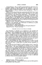
Figure 5.3.6-138 Mach Contours from Panel 8/9 T-Seal Damage Coupled External/Internal Flow 

Simulation (15 million-cell Model; Postprocessed using every other points) 

Figure 5.3.6-139 Mach Contours from Panel 8/9 T-Seal Damage Coupled External/Internal Flow 

Simulation (15 million-cell Model; Postprocessed using every other points) 

NSTS-37398 AeroAerothermalThermalStructuresTeamFinalReport.pdf 

458 

R EPORT V OLUME V OCTOBER 2003 

444 

CTF091-0450


COLUMBIA 


Figure 5.3.6-140 Pressure Contours on Earmuff Insulation and Rib Channel from Panel 8/9 T-Seal 

Damage Coupled External/Internal Flow Simulation ( 2 million-cell Model) 

Figure 5.3.6-141 Heating Contours on Earmuff Insulation and Rib Channel from Panel 8/9 T-Seal 

Damage Coupled External/Internal Flow Simulation ( 2 million-cell Model) 


445 

CTF091-0451 

R EPORT V OLUME V OCTOBER 2003 459


COLUMBIA 


Figure 5.3.6-142 Pressure Contours on Earmuff Insulation and Rib Channel from Panel 8/9 T-Seal 

Damage Coupled External/Internal Flow Simulation (15 million-cell Model) 

Figure 5.3.6-143 Heating Contours on Earmuff Insulation and Rib Channel from Panel 8/9 T-Seal 

Damage Coupled External/Internal Flow Simulation (15 million-cell Model) 


460 


446 

CTF091-0452


COLUMBIA 


Figure 5.3.6-144 BHB Panel8/9 T-seal Damage Internal Streamtraces 

5.3.6.2.4 BRPP 3-D Panel 8/9 Damaged T-Seal Solution 

5.3.6.2.4.1 Case Description 

The first objective of this effort was to compute convective heating rates on key surfaces of the Leading 

Edge Structural Subsystem (LESS) for the scenario of a damaged T-Seal in the RCC 8/9 location. These 

included: 

• RCC T-Seal 

- Cavity 

- Rib channel 

• Internal insulation units: 

- Forward spar insulator units (hot tubs) 

- Spanner Beam Insulator units (earmuffs) 

The T-Seal damage was assumed to be a piece missing from the intersection of the T-Seal and the lower 

edge of the earmuff to the geometric leading edge as shown in Figure 5.3.6-145. 


447 

CTF091-0453 



COLUMBIA 


Figure 5.3.6-145 – Damaged T-Seal Geometry 

The intended application of the data was to enhance the engineering heat transfer models and to improve 

understanding of this flow field structure. The second objective of this effort was to construct an accurate 

CAD model of the LESS components that would serve as a universal model usable for all types of 

multidimensional analysis via IGES export. This would possess clean, “watertight”, trimmed surfaces for 

import to modeling software. 

5.3.6.2.4.2 Grid/Solution Development 

The universal CAD model was constructed with the Pro/Engineer parametric CAD system. Sources for 

geometry included imported CAD models for the RCC panels, forward wing spar, and RCC attachment 

brackets. Design specifications combined with photographs were used for the earmuffs, hot tubs, and wick 

insulators. No detailed drawings for the latter three components have been located to date. The model 

has been completed however issues precluded its use for CFD grid generation. The imported RCC parts 

were too complex for analysis use. They contained over 1,000 surfaces per RCC panel as well as 

duplicate surfaces. In addition, the model architecture requires a large amount of prep work prior to export 

for analysis grid generation due to the grouping of surfaces with solids. It was anticipated that an 

additional 1-2 weeks would be required to complete this task. A fallback plan was implemented in which 

development of the universal CAD model would continue, while the NASA JSC-based model for internal 

region used in for the 10” Leading Edge Breach would be modified for use in this analysis. The T-Seal 

channel geometry was extracted from the Pro/E CAD model and integrated into the JSC model (Figure 

5.3.6-145). As discussed in Section 5.3.6.1.4, the JSC model included the RCC 7/8, 8/9, 9/10 earmuffs 

and the hot tubs in between them. The negative aspect of this model was that all of the edges were sharp, 

which conflicted with other models and photographs. Dimensions of key components, such as the 

earmuffs and hot tubs, were also somewhat uncertain since the JSC dimensions conflicted with a model 

used by Boeing Huntington Beach and some photographs. 


462 


448 

CTF091-0454


Earmuffs 

JSC model 

COLUMBIA 


Pro/E Universal model 

Hot tub 

Earmuff 

Hot tub 

Earmuff 

Figure 5.3.6-146 – Internal Region Geometry Models 

JSC model with 

RCC panels 

removed 

The JSC and the Pro/E Universal model are compared in Figure 5.3.6-146. Extruded “dump” regions were 

added on either side of RCC 8 and 9 to enable the application of constant pressure outflow boundary 

conditions. The dimensions of these regions were based on the results of the 2-D T-Seal analysis of 

Sec.5.3.6.2.2. 

Previous analyses had shown that a high degree of coupling existed between the internal and external 

flow fields. A NASA LaRC LAURA external flow solution was used to provide the necessary coupling, but 

only a small three-zone portion of it. This was carefully selected to reduce the size of the model while 

preserving the external solution in the region of interest (Figure 5.3.6-147). Not all of Zone 36 was 

required so it was sectioned with a cutting-plane interpolation. 

Zone 36 

Zone 37 

Zone 38 

Figure 5.3.6-147 - LAURA Solution Zones Used as External Domain 


449 

CTF091-0455 



The Boeing APPT system was used to generate the hybrid viscous unstructured computational grid. The 

unstructured approach greatly reduces the time required to generate the grid and eliminates wasted 

clustering cells in complex internal regions. After a number of revisions, final grids (Figure 5.3.6-148) were 

produced containing 4.1M elements with a wall spacing of 1.0e -4 inches, and 5.7M elements with a wall 

spacing of 1.0e -5 inches. Results from the 2-D T-Seal analysis (Sec. 5.3.6.2.2) along with a cardboard 

model and discussion among compressible flow experts were used to determine the clustering of elements 

in the internal region. 

Internal region 

with some 

RCC 

components 

removed 

Earmuff and 

RCC rib detail 

RCC RCC 88 

Earmuff Earmuff 

Hot Hot tub tub 

RCC RCC 99 

Figure 5.3.6-148 – Hybrid Viscous Unstructured Grid 

Broken T-Seal 

detail 

The solutions were obtained using the Boeing ICAT code. Fully laminar flow was assumed based on the 

extremely low Reynolds numbers present. Liu-Vinokur equilibrium air thermochemistry and Tannehill 

transport properties were used. The convergence criteria were to drive net fluxes to an initial steady-state 

and also to drive integrated heat load in key areas to steady-state. Contours of heat flux in key areas were 

also plotted at different time steps. 

The CFD Condition 1 trajectory point was used to define the freestream conditions. All wall temperatures 

were set to 3,000º R. This corresponds to the melting temperature for the Inconel 601 outer layer of the 

Dynaflex surfaces such as the earmuffs and hot tubs. The pressure on the cavity outflow surfaces was set 

according to Table 5.3.6.1-1. These values were established from venting analysis. Note that the values 

have evolved over time as has the venting analysis. The current level of 10.8 psf (517 Pa) is the result of 

the 2-D T-Seal computations being fed back into the venting analysis. 

5.3.6.2.4.3 Results 

COLUMBIA 


5.3.6.2.4.4 Major flow structure comments 

Figure 5.3.6-149 shows the flow inside the LESS cavity. The walls are colored by static pressure, and the 

streamlines are colored by Mach number and are launched from the center of rib channel. Subsonic flow 

is observed exiting the rib channel into the LESS cavity. This is due to the high cavity backpressure of 

.075 psia vs. ~.060 psia at the rib channel exit. The latter number comes from examination of the T-Seal 

2-D solutions (Sec. 5.3.6.2.2) and represents the rib channel exit pressure without the influence of 

backpressure. Overexpanded laminar flow, such as this, easily separates, and normal shock structures 

reduce the flow to subsonic and also reduce total pressure. Both of these effects reduce the capability of 

the flow to generate heat flux on impingement surfaces. The majority of the LESS cavity flow is largescale 

subsonic vortices. 


464 


450 

CTF091-0456


Figure 5.3.6-150 shows the flow in the RCC rib channel. Again, the walls are colored by static pressure, 

and the streamlines are colored by Mach number, however this time they are launched from a boundary 

layer rake in the external flow. This flow field has features similar to the 2-D T-Seal solutions (Sec. 

5.3.6.2.2). These include the aerodynamic throat, the upstream edge separation, and the downstream 

edge bow shock. Surface pressures are also close to the 2-D solutions. 

RCC 7/8 earmuff 

RCC 8/9 earmuff 

RCC 8 hot tub 

RCC RCC 8/9 8/9 ribs ribs 

Figure 5.3.6-149 - Mach-colored Cutting Plane and Wall Static Pressure Detail View From in Front of 

Leading Edge 

Aerodynamic 

throat 

Upstream 

edge 

separation 

COLUMBIA 


Bow shock 

Figure 5.3.6-150 – View Into RCC Rib Channel 


451 

CTF091-0457 



5.3.6.2.4.5 Surface heating and pressure comments 

Figure 5.3.6-151 shows surface heat flux in the region where the RCC 8/9 earmuff and the RCC 8 hot tub 

intersect. This is the area of highest heating on the earmuff and hot tub surfaces, as would be expected 

based on the pressure and Mach fields observed. The levels are low compared to the peaks observed for 

the 2-D T-seal solution (Sec. 5.3.6.2.2) where supersonic flow is impinging on the earmuff. Heat fluxes in 

the rib channel closely match the USA 2-D T-Seal solutions (Sec. 5.3.6.2.2). The medium grid solution 

was run a total of 28,000 time steps. The solution was monitored periodically using flow visualization. No 

indication of unsteady flow was found, however there is still a possibility that this could occur. Many more 

time steps would be needed to be certain. 

RCC RCC 8 8 hot hot tub tub 

COLUMBIA 


RCC RCC 8/9 8/9 

earmuff earmuff 

RCC RCC 8/9 8/9 ribs ribs 

Figure 5.3.6-151 - Surface Heat Flux Detail View From in Front of Leading Edge 


466 


452 

CTF091-0458


5.3.6.3 CFD of Simplified Internal Wing Geometry 

5.3.6.3.1 Methodology and Philosophy of “Insight CFD” 

CFD was used not only to help characterize fine details in the flow field with large, detailed CFD models, 

but also to help understand some of the larger scale flow phenomenon. For this purpose a few large scale, 

simplified models were created to understand the flow patterns once a breach of the internal wing cavity 

was initiated. These models were primarily used to visualize flow patterns within the wing cavity. They 

were not relied upon for detailed information such as wall heat fluxes, heat transfer coefficients, surface 

temperatures, or transient calculations. 

Two simplified models were created. The first was a simplified model of the entire left wing aft of the 1040 

wing spar and without the wheel well cavity. Wing spar designations are shown in Figure 5.3.6-153 for 

reference. This model did not include the RCC cavity along the wing leading edge. The purpose of this 

model was to visualize the flow field within the wing cavity immediately after the leading edge spar breach. 

This model assumed that the flow coming onto the wing cavity was normal to the spar. The second 

“insight” CFD model was a 2-D model of the left wing cavity and the RCC cavity. This model was used to 

visualize the flow through the RCC breach, through the wing spar breach, then into the wing cavity directly 

outboard of the wheel well. The purpose of this model was to verify whether or not it was possible for the 

flow to come into the wing cavity normal to the leading edge spar or not. 

Models are “simplified” in the sense that only the necessary surfaces needed to characterize the flow field 

satisfactorily are included. The 3-D wing model has none of the internal circular struts connecting the 

upper and lower wing surfaces. Only the internal spars and spar vents and the wing upper and lower 

surfaces are included. The wing upper and lower surfaces were generated based solely on the spar 

outlines; therefore some of the finer details in the wing curvature were not captured in the models. All walls 

within the models are smooth walls, which in reality is not the case, particularly in the area of the wheel 

well walls. 

FLUENT 6.1 was the CFD code used to model these simplified geometries. FLUENT 6.1 is a commercial 

Navier-Stokes solver for unstructured meshes. It is a cell-centered, finite-volume code. FLUENT's three 

solvers can be used to compute the flow and heat transfer for all flow regimes, from low subsonic via 

transonic and supersonic to hypersonic. The unstructured grid capability in FLUENT allows for modeling of 

complex geometries similar to the geometry found in the wing and wheel well areas of Columbia. A more 

detailed description of FLUENT can be found in the Appendix and in [1]. 

5.3.6.3.2 3-D Solution Cases 

COLUMBIA 


5.3.6.3.2.1 3-D Wing Model, 6 inch and 10 inch Spar Breach 

The purpose of the analysis was to determine the flow path of the plume entering the wing through the 

wing leading edge spar. A steady state analysis was done using boundary conditions corresponding to the 

time immediately following the wing spar breach, approximately 490 seconds after entry interface. 

A simplified model of the left wing of Columbia was created, Figure 5.3.6-152, and shows the outer wall 

boundaries of the model including the wing upper and lower surfaces and the leading edge spar. A circular 

breach hole was located in the wing spar leading edge at the intersection of RCC panels 8 and 9. Two 

different spar breach hole diameters were modeled - circular breach sizes of 6 inches and 10 inches 

diameter were chosen based upon other analyses performed as part of the investigation. An assumption 

was made that the flow coming into the wing area would be normal to the spar. 

Figure 5.3.6-153 shows the internal spars and vents not visible in Figure 5.3.6-152. Three flow exit areas 

are included in the wing model and are shown in Figure 5.3.6-153. A rectangular vent area of 180 in 2 is 

located in the 1040 wing spar. The internal wing volume forward of the 1040 spar was not included in the 

model, instead pressures obtained from the MSFC analyses outlined in Section 5.3.5.7 were used to set 

the conditions at that interface. The other two flow exits are located at the rear of the model at the 1365 

spar location. These vents are located at the approximate locations where the inboard and outboard 

elevons penetrate the 1365 spar. Vent areas were 2.55 in 2 and 5.5 in 2 for the inboard and outboard 


453 

CTF091-0459 



COLUMBIA 


elevons, respectively. Four internal vents allow for flow between the various internal wing compartments 

and are shown along with their areas in Figure 5.3.6-153. 

The wing geometry was simplified in order to reduce the computational expense of the model. None of the 

tubular struts supporting the upper and lower wing surfaces were included in the model. As mentioned 

previously, the wing volume forward of the 1040 spar was not included. The wheel well volume was not 

included due to the complex geometry in the wheel well and because the primary focus of the analysis was 

flow paths within the wing, not the wheel well area. Another area of simplification was the wing surfaces. 

These were not imported directly from CAD geometry, but were created within the FLUENT geometry 

generation program. This means that there may be subtle differences between the FLUENT wing surfaces 

and the actual wing surface geometry, however due to the overall size of the model it is not anticipated that 

this difference would have a significant effect on the results. The size of the 3D wing model computational 

domain was approximately 340,000 cells. 

Boundary conditions for the 3-D model are shown in Figure 5.3.6-154 for the 6-inch breach case and in 

Figure 5.3.6-155 for the 10-inch breach case. Pressure boundary conditions were applied at the breach 

hole and three flow exit boundaries. These pressure values were obtained from the MSFC venting model 

discussed in Section 5.3.5.7. The pressures correspond to the boundary pressures at 500 seconds after 

entry interface. This time is 10 seconds after the estimated spar breach time of 490 seconds. 

The standard k-e turbulence model available in FLUENT was activated for all of the 3-D and 2-D analyses. 

The working fluid was air modeled as an ideal gas. No attempt was made to model the chemical reactions 

occurring within the gas at these elevated temperatures using FLUENT. A correlation for determining the 

specific heat of air as a function of temperature from 495 o R to 10400 o R was used in the all of the 2-D and 

3-D FLUENT models due to the large variation of specific heat over this temperature range. This 

correlation was input into FLUENT as a piecewise-polynomial function, and a plot of this correlation versus 

the data used to generate it can be found in Figure 5.3.6-156. The models were run until convergence was 

met on the net mass flow in and out of the domain, and pressures reached a steady state value. 

5.3.6.3.2.2 Results – 3D Model, 6 inch Breach hole 

Results of the 3-D internal wing flow case with a 6-inch diameter spar leading edge breach are shown in 

Figure 5.3.6-157 through Figure 5.3.6-161. Figure 5.3.6-157 is a contour plot of velocity magnitude on a 

plane cut horizontally through the entire wing. The plot shows that the flow does not penetrate significantly 

beyond the 1191 spar, and that it tends to circulate within the cavity outboard of the wheel well and exit 

through the 1040 spar vent. Some flow does penetrate all the way to the rear elevon vents, and Figure 

5.3.6-158 shows this with a velocity contour plot with a different scale. 

Mass flow rates and Mach numbers for the flow inlet and three flow exits are shown in Table 5.3.6.3-1. The 

mass flow rates indicate that 78% of the incoming gas exits the wing cavity through the 1040 spar vent. 

Table 5.3.6.3-1 6-inch Breach Hole Mass Flow Rates and Mach Numbers 

Vent Mass Flow Flow Mach 

Lb/min direction Number 

6” Dia breach Hole 0.686 In 1.06 

1040 Spar Vent 0.535 Out 0.105 

Inboard elevon 0.0667 Out 0.83 

Outboard elevon 0.0835 Out 0.39 

Figure 5.3.6-159 shows pathlines (colored by velocity magnitude) to indicate the flow paths of hot gas 

entering the wing cavity. The pathlines begin at the breach hole location. The flow impinges directly on the 

outboard wheel well wall then turns 180 degrees and the majority of the flow exits through the 1040 vent 

hole. A small percentage of the flow does penetrate all the way to the rear of the wing but at a much slower 

velocity than seen in the cavity outboard of the wheel well. 


468 


454 

CTF091-0460


COLUMBIA 


Figure 5.3.6-160 shows a contour of static pressure within the wing. The figure indicates that the pressure 

at the 1040 spar vent drives the resulting static pressure. This is due to the large size of that vent in 

relation to the two smaller rear vents. Figure 5.3.6-161 shows a contour plot of static temperature within 

the wing. 

5.3.6.3.2.3 3D Model, 10 inch Breach hole 

Results of the 3-D internal wing flow case with a 10-inch diameter spar leading edge breach are shown in 

Figure 5.3.6-162 through Figure 5.3.6-166. Figure 5.3.6-162 and Figure 5.3.6-163 are contour plots of 

velocity magnitude on a plane cut horizontally through the entire wing using two different scales to help 

visualize both the higher speed flow outboard of the wheel well and the low speed flow rear of the 1191 

spar. The plots shows that even with the higher energy flow coming in the breach, the flow still does not 

penetrate significantly beyond the 1191 spar. Table 5.3.6.3-2 lists the mass flow rates and Mach numbers 

that again indicate that the majority of the flow (87%) entering the wing exits forward through the 1040 spar 

vent. 

Table 5.3.6.3-2 10-inch Breach Hole Mass Flow Rates & Mach Numbers 

Vent Mass Flow Flow Mach 

Lb/min direction Number 

6” Dia breach Hole 7.13 In 1.06 

1040 Spar Vent 6.19 Out 0.75 

Inboard elevon 0.29 Out 0.95 

Outboard elevon 0.65 Out 0.95 

Figure 5.3.6-164 shows pathlines (colored by velocity magnitude) to indicate the flow paths of hot gas 

entering the wing cavity. The flow impinges directly on the outboard wheel well and exits primarily through 

the 1040 vent hole, similar to the 6-inch breach case. As in the 6-inch breach case some flow penetrates 

the cavity aft of the 1191spar. Figure 5.3.6-165 shows a contour of static pressure within the wing. Figure 

5.3.6-166 shows a contour plot of static temperature within the wing. Comparing the temperature contour 

plots between the 6-inch breach (Figure 5.3.6-161) and the 10-inch breach case (Figure 5.3.6-166), the 

area behind the 1191 spar is much warmer in the 10-inch case. The larger breach hole size is able to push 

more flow beyond the 1191 spar vent into this region. 

5.3.6.3.3 2-D Simplified Wing Model Solutions 

The purpose of the analysis was to trace the flow path of the plume as it enters the RCC cavity and 

impinges on the RCC attach hardware, then passes through a breach hole in the wing spar. It was 

assumed that the plume would be deflected by the RCC attach hardware and burn a hole through the 

spar, entering the wing cavity in the direction approximately normal to the spar. The analysis is an attempt 

to support the 3-D model assumption that flow is entering the wing cavity normal to the spar. A steady 

state analysis was done using boundary conditions corresponding to the time immediately following the 

wing spar leading edge breach, approximately 490 seconds after entry interface. 

A simplified 2-D model of the left wing of Columbia was created and is shown in Figure 5.3.6-167. The 

view is looking up from below the left wing. The model consists of the wing cavity bounded by the wheel 

well outer wall, the 1040 spar, the 1191 spar, and the leading edge spar. This wing geometry was derived 

from the 3-D model. A section representing the RCC cavity was added along the length of the wing leading 

edge spar. The 2-D RCC cavity geometry was approximated with a 29-inch deep channel. A 10-inch 

diameter hole was located on the leading edge of the RCC cavity in the approximate location of panel 8. 

The green lines shown in Figure 5.3.6-167 represent interior zones in the domain and are not hard walls. 

Four flow exit areas are included in the wing model. A pressure outlet is located in the 1040 wing spar, and 

another pressure outlet represents the vent in the 1191 spar that allows flow to pass to the rear cavities of 

the wing. The RCC cavity has two pressure outlets located at either end of the RCC cavity. These 

openings were sized based upon leakage areas obtained from the MSFC venting model discussed in 

Section 5.3.5.7 


455 

CTF091-0461 



Figure 5.3.6-167 also shows the simplified RCC attach hardware used in the model. The attach hardware 

(representing the spanner beam insulation) in the model represents the hardware associated with RCC 

panel #8, and the breach hole in the spar is located directly adjacent to this attach hardware. 

Boundary conditions for the 6 inch and 10 inch breach hole 2-D models are shown in Table 5.3.6.3-3. 

Static pressure boundary conditions were applied at the four flow exit boundaries. These pressure values 

were obtained from the MSFC venting model discussed in section 5.3.5.7. The pressures correspond to 

the boundary pressures at 500 seconds after entry interface. 

RCC Leading 

Edge Breach 

Table 5.3.6.3-3 2-D Model Boundary Conditions 

Breach 

Pressure 

Lb/ft 2 

COLUMBIA 


Breach 

Temperature 

o R 

1040 Spar 

Vent 

Lb/ft 2 

1191 Spar 

Vent 

Lb/ft 2 

RCC Fwd 

Vent 

Lb/ft 2 

RCC Rear 

Vent 

Lb/ft 2 

6 inches 37 6000 0.92 1.04 13.2 13.2 

10 inches 37 6000 8.6 9.65 13.2 13.2 

The flow entering the RCC cavity was redirected to impinge directly at the corner of the RCC attach 

hardware. This assumption was supported by other coupled external/internal CFD analyses which show 

the RCC inlet plume impinging directly on the corner of the attach hardware. All walls of the domain were 

set at a constant temperature of 50 o F, and the same turbulence models and specific heat correlations 

were used as in the 3-D models. 

5.3.6.3.3.1 2-D Results - 6 inch Spar Breach 

Results of the 2-D internal wing flow case are shown in Figure 5.3.6-168 and Figure 5.3.6-169. The 

velocity contour plot of Figure 5.3.6-168 shows the flow does penetrate the spar approximately normal to 

the spar. This figure as well as the pathlines of Figure 5.3.6-169.shows how the spanner beam insulation 

hardware turns the flow. Both plots support the assumption made in the 3-D model that initially the flow 

coming into the wing cavity was normal to the spar. There are some differences in the flow patterns 

compared with the 3-D model results, and this is likely due to the restrictions on the flow imposed by the 2- 

D geometry. In the 3-D case the flow can circulate around the wing cavity by splitting and traveling over 

and under the incoming jet, while in the 2-D model the flow is blocked from doing this by the incoming jet. 

The flow direction into the wing cavity at a later time would depend upon the length of time that the RCC 

attach hardware remained in place. 

5.3.6.3.3.2 2-D Results - 10 inch Spar Breach 

Results of the 2-D internal wing flow case are shown in Figure 5.3.6-170 and Figure 5.3.6-171. As in the 6inch 

wing spar breach case, the velocity contour plot of Figure 5.3.6-170 shows the spanner beam 

insulation hardware turns the flow so it enters the wing approximately normal to the spar. This is also 

indicated in the pathline plot of Figure 5.3.6-171. Both plots support the assumption made in the 3-D model 

that initially the flow coming into the wing cavity was normal to the spar. 


470 


456 

CTF091-0462


Vent, 408.5 in 2 

Vent, 397.6 in 2 

1040 Spar Vent 

180.1 in 2 

Spar breach hole 

Figure 5.3.6-152 3-D Simplified Wing Geometry 

Vent, 404.6 in 2 

1191 Spar 

Wheel well wall 

COLUMBIA 


1365 Spar 

Inboard elevon 

2.55 in 2 (circular hole) 

Wing leading edge spar 

Figure 5.3.6-153 3-D Model Vent sizes 


Outboard elevon 

5.5 in 2 (circular hole) 

Vent, 404.6 in 2 

Breach hole (6 in, 10 in diameter) 

457 

CTF091-0463 



8.57 lb/ft 2 

2.67 lb/ft 2 

COLUMBIA 


1.37 lb/ft 2 

9.9 lb/ft 2 , 6000 o R 

2.4 lb/ft 2 

All walls set at 50 o F 

Constant temperature 

Figure 5.3.6-154 6-inch Breach Hole Boundary Conditions 

2.29 lb/ft 2 

37.1 lb/ft 2 , 6000 o R 

5.26 lb/ft 2 

All walls set at 50 o F 

Constant temperature 

Figure 5.3.6-155 10-inch Breach Hole Boundary Conditions 


472 


458 

CTF091-0464


COLUMBIA 


Figure 5.3.6-156 Specific Heat of Air Curve Fit used in FLUENT CFD Cases 

Figure 5.3.6-157 6-inch Breach hole, Velocity Contour Plot 


459 

CTF091-0465 



COLUMBIA 


Figure 5.3.6-158 6-inch Breach Hole, Velocity Contour Plot 

Figure 5.3.6-159 6-inch Breach Hole, Pathlines 


474 


460 

CTF091-0466


COLUMBIA 


Figure 5.3.6-160 6-inch Breach Hole, Static Pressure 

Figure 5.3.6-161 6-inch Breach Hole, Static Temperature 


461 

CTF091-0467 



COLUMBIA 


Figure 5.3.6-162 10-inch Breach Hole Velocity Contours 

Figure 5.3.6-163 10-inch Breach Hole Velocity 


476 


462 

CTF091-0468


COLUMBIA 


Figure 5.3.6-164 10-inch Breach Hole, Pathlines 

Figure 5.3.6-165 10-inch Breach Hole, Static pressure Contours 


463 

CTF091-0469 



Figure 5.3.6-166 10-inch Breach Hole, Static Temperature Contours 

1040 spar vent 

1191 spar vent 

COLUMBIA 


RCC outlet 

6 inch and 10 inch 

wing spar breach 

10 inch breach 

in leading edge 

Wing cavity 

Spanner beam insulation, 

RCC panel 8-9 I/F 

RCC cavity 

RCC outlet 

Figure 5.3.6-167 2-D Model Geometry – 10 inch Breach in RCC Leading Edge, 6 and 10-in Spar 

Breach 


478 


464 

CTF091-0470


COLUMBIA 


Figure 5.3.6-168 2-D Model, 6-inch Breach in Wing Spar, Velocity Contours 

Figure 5.3.6-169 2-D Model, 6-inch Breach in Wing Spar, Pathlines 


465 

CTF091-0471 



COLUMBIA 


Figure 5.3.6-170 2-D Model, 10-inch Breach in Wing Spar, Velocity Contour 

Figure 5.3.6-171 2-D Model, 10-inch Breach in Wing Spar Pathlines 

5.3.7 Application of Data to the Working Scenario 

5.3.7.1 Plume impingement angle in WLE 

The insight provided by the CFD results for RCC penetrations with coupled flow fields allowed the 

adjustment of the assumed jet internal direction from normal to the interior surface to an angle reflective of 

the transverse momentum ingested into the RCC penetration. Figure 5.3.7-1 displays the two-inch 

penetration solution in RCC panel 6 by Peter Gnoffo. The streamlines turn into the hole initially at a 20degree 

angle, that then interacts with the downstream lip shock resulting in a final flow turning angle of 41 

degrees. It is desired to take advantage of this solution to generalize the internal jet direction to any 

penetration location. In doing so, the panel 6 results are assessed for a simple correlating parameter. A 


480 


466 

CTF091-0472

local velocity based coordinate system is defined, as shown in Figure 5.3.7-1, with one component aligned 

with the velocity vector at the boundary layer edge and the other along the inward normal to the surface. 

Directional components were then assigned to the vectors. Many combinations of momentum components 

were tried, but with the uncertain impact of the lip shock, a simple correlation of boundary layer edge 

dynamic pressure (qe) and surface static pressure (pe) was chosen. The initial 20-degree flow turning angle 

was well reproduced with the ratio of static pressure over average ingested dynamic pressure. Boundarylayer 

edge properties are used to simplify the application to the entire wing. Figure 5.3.7-2 shows the 

process used to derive the correlation parameter, C, to apply to the edge properties in establishing the flow 

turning into a penetration. Therefore, once the local coordinates are established, the predicted internal jet 

direction can be calculated as 

r 

( 0 . × q ) V + p P 

J = 176 e e 

With this definition established, a series of points along the projected debris path were chosen as 

illustrated in Figure 5.3.7-3 with the symbols. The J vectors are represented in three dimensions in the 

accompanying views of Figure 5.3.7-3, with the view from inboard on top and the view looking down on the 

RCC outlines on the bottom. Due to the double delta shape of the Orbiter wing, and the projected impact 

path at the juncture, the vectors primarily point to the spar region behind panel 8.In Figure 5.3.7-4 a 

representation of the RCC insulation system has been added in investigating the impact points of the 

selected jet penetrations. Due to the vector alignment and insulation configuration the conclusion is that 

the most likely primary impingement location for an RCC penetration along the predicted foam path is the 

spar region behind panel 8 or the earmuff region between panels 8 and 9. Table 5.3.7.1-1 provides the 

selected penetrations and the associated jet direction unit vectors. 

_ 

V 


COLUMBIA 


Figure 5.3.7-1 Panel 6 penetration and Jet direction coordinate system. 


r 

_ 

P 

r 

467 

CTF091-0473 



COLUMBIA 


Figure 5.3.7-2 Jet direction correlation parameter derivation 

Figure 5.3.7-3 Selected penetration locations and projected plume directions 


482 


468 

CTF091-0474


COLUMBIA 


Figure 5.3.7-4 Jet penetration assessment 

X Y Z JetX JetY JetZ 

1087.40 226.40 283.69 0.773 0.185 0.607 

1088.09 221.74 282.61 0.775 0.173 0.608 

1085.12 224.67 283.66 0.775 0.178 0.606 

1082.34 226.31 284.54 0.776 0.179 0.605 

1085.03 222.34 283.15 0.776 0.173 0.607 

1084.47 218.03 282.33 0.777 0.165 0.607 

1082.20 221.60 283.44 0.778 0.169 0.605 

1079.10 223.87 284.55 0.779 0.169 0.603 

1077.42 221.25 284.19 0.780 0.164 0.604 

1079.82 217.54 282.90 0.780 0.159 0.605 

1075.67 216.60 283.35 0.782 0.156 0.604 

1074.39 220.23 284.52 0.783 0.157 0.602 

1069.58 222.38 286.20 0.778 0.164 0.606 

1071.82 218.29 284.50 0.784 0.151 0.602 

1071.67 214.38 283.50 0.784 0.149 0.603 

1067.86 213.76 284.04 0.786 0.145 0.601 

1069.25 215.53 284.25 0.785 0.147 0.601 

1064.78 218.99 286.31 0.785 0.149 0.601 

1062.50 215.94 285.84 0.785 0.149 0.602 

1065.37 212.72 284.25 0.788 0.141 0.600 

1061.87 210.19 284.23 0.790 0.137 0.598 

1058.09 213.32 286.04 0.792 0.135 0.596 

1066.90 210.78 283.45 0.787 0.142 0.601 

1058.65 208.86 284.49 0.792 0.134 0.596 

1054.96 211.26 286.07 0.794 0.129 0.594 

1051.40 211.92 287.24 0.797 0.121 0.592 

1054.82 214.19 287.20 0.796 0.124 0.592 

1050.94 209.88 286.56 0.797 0.122 0.591 

1054.97 205.85 284.35 0.794 0.130 0.594 

1057.20 206.49 284.10 0.793 0.132 0.595 

1049.54 208.27 286.30 0.798 0.121 0.591 

1045.30 210.44 288.34 0.801 0.104 0.590 

1047.57 212.37 288.55 0.803 0.102 0.588 

1046.34 206.93 286.58 0.798 0.119 0.590 

1043.32 206.24 287.06 0.800 0.114 0.589 

1041.77 207.76 288.11 0.806 0.104 0.583 

1040.48 202.72 286.38 0.802 0.107 0.588 

1036.79 205.16 288.31 0.810 0.087 0.581 

1040.43 203.92 286.85 0.801 0.108 0.589 

1046.73 205.56 285.99 0.797 0.119 0.591 

1050.73 202.89 284.32 0.795 0.126 0.593 

1056.37 207.78 284.63 0.793 0.132 0.595 

Table 5.3.7.1-1Jet penetration directions 

5.3.7.2 Plume heating distribution 

As the investigation team narrowed in on a preferred working scenario, the internal flow team was asked to 

pull together internal heating distributions for assumed penetration locations that incorporate not only the 

primary impingement heating, like that described in 5.3.3.2, but also convective heating rates to the 


469 

CTF091-0475 



COLUMBIA 


surrounding internal TPS surfaces. Based on an assumed hole location and size, internal plume 

impingement environments were created that incorporate heating distributions for the panel 8/9 region 

based on assumed internal direction (5.3.7.1), degree of secondary splash heating, and geometric flow 

shadowing effects. Full 3-D CFD results for panel 7/8 penetrations were not yet complete, so the best fully 

coupled CFD solution with internal heating was used as a basis. Given the degree of engineering involved 

in producing the environments, uncertainty values of +/- 50% were applied to the final results and 

additional comparisons to higher fidelity CFD results were pursued to provide independent assessment of 

the expected internal heating. 

5.3.7.2.1 Selection of assumed hole location 

The present working scenario includes penetration of RCC from panels 6-9 with subsequent spar breach 

at 488 seconds from entry interface. The team chose a single penetration location for complete analysis in 

order to ballpark the hole size required to match the flight data for the panel 9 spar and clevis temperature 

measurements and the spar breach time of 488 seconds from E.I. Given similar heating analysis 

completed early in the investigation using the basic MMOD plume model, 5.3.3.2, hole sizes of 4, 6, and 

10 inches in diameter were chosen and anticipated to bound the data. Hole location was chosen to 

maximize the predicted primary impingement heating rate, based on the internal flow direction analysis of 

5.3.7.1. Using the simple 1-D plume heating model, the plume vectors of Table 5.3.7.1-1 were assessed 

and vector # 18 chosen and colored red in Figure 5.3.7-5. The anticipated heating rates at the primary 

impingement point are increased both by the short distance to the earmuff and the small radius of 

curvature on the TPS edge. The coordinates of the assumed penetration are X=1065 in, y=-219 in, and z= 

286.3 in. 

Figure 5.3.7-5 Panel 8 lower surface penetration location 

5.3.7.2.2 Distribution methodology 

Internal heating distributions are based on a modification of the baseline engineering methodology for 

holes as outlined Section 5.3.3.3 and take advantage of ingested flow enthalpy calculates using the 

methodology in Section 5.3.2 and a computed internal pressure using the methodology of Section 5.3.5. 

The local axis of the plume is assumed to align along the predicted direction of 5.3.7.1, independent of the 

hole diameter. This assumption was made due to the lack of available internal CFD at the time. (In truth, 

the larger holes will allow more transverse momentum to enter the hole and cause the jet to hug the 

interior RCC surface more than the present methodology based on 2” diameter hole results, but the 

heating distribution will only be shifted in space with little impact on peak heating values.) The radial 

position correction of the baseline methodology is replaced with computed three-dimensional factors as a 

function of hole size, which are presented in the results section below. Trajectory corrections remain the 

same, resulting in a final equation of 

q& 

q ( t) 

V ( t) 

q& × & 

( 488) 

∞ 

∞ 

( x y, 

z, 

t, 

d ) = ( x, 

y, 

z, 

d ) × × q ( d ) 

, hole q& 

hole 

2 

plate 

q∞ 

( 488) 

V ∞ 

The baseline heating values, qplate, are given for each hole size, computed for a trajectory time of 488 

seconds from E.I., in Table 5.3.7.2-1. 


484 


2 

plate 

hole 

470 

CTF091-0476


COLUMBIA 


10” Hole 55.9 Btu/ft 2 sec for plate 



Table 5.3.7.2-1 Panel 8 penetration heating values 

5.3.7.2.3 Correlation and geometry correction factors 

The methodology was adjusted based on the LAURA 2” diameter hole panel 6 penetration calculation of 

Section 5.3.6.1.4.1. Interior surface heating rates are extracted for the primary impingement region and the 

secondary splash surface. Corrections to the baseline model are made to bring the results into line with the 

CFD results. Comparison lead to a narrowing of the distribution by raising the values of Table 5.3.3.3-1 to 

the 1.6 power (also indicated by the comparisons in Figure 5.3.3-7) and the development of a splash 

heating approach to account for flow turning and secondary stagnation flows anticipated in the RCC cavity. 

Examination of the LAURA results indicated flow physics similar to a forward-facing step. Forward-facing 

step amplifications of 3.5 times the undisturbed value are appropriate for the observed internal Mach 

numbers and produced a good comparison on the splash surface of Figure 5.3.7-6. Secondary stagnation 

values are within 20% and the engineering methodology remains conservative as the flow moves down the 

surface. 

In addition to secondary splash factors, other corrections to the baseline methodology are applied to 

account for “shadowing,” where the flow cannot directly impinge on the surface, local surface radius of 

curvature effects to earmuff edges and a general convective heating equal to three percent of peak values. 

The final geometry corrections are presented in Figure 5.3.7-7. Spar and carrier panel surfaces behind 

panel 8 are assumed to be secondary splash surfaces with a preference for the flow to splash on the upper 

surface and hence have amplification factors from 1 to 3.5. The edge of the panel 8/9 earmuff facing the 

assumed breach location shows high amplification factors to correct for local radius of curvature effects. 

The region behind panel 9 cannot be directly impinged upon from the assumed location and therefore has 

shadowing corrections that decrease the heating. 

Figure 5.3.7-6 Comparison of 3D methodology with LAURA calculations with LAURA 


471 

CTF091-0477 



• Corrections given on a zone by 

zone basis to partially account 

for 

1. Secondary splash surface 

(based on forward facing step and 

panel 6 hole comparisons) 

2. Radius of curvature 

corrections to modeled 

geometry (Spanner beam 

insulation modeled with square 

corners, corrected to 1” radius 

heating) 

3. Line of sight shadowing and 

separation (panel 9 spar heating) 

4. Background heating values 

of 3% assumed on backward 

facing surfaces (on par with 

panel 6 and T-seal simulations) 

COLUMBIA 


Figure 5.3.7-7 Geometry correction for heating 

5.3.7.2.4 Resulting Distributions 

Engineering predicted heating distribution factors are presented in Figure 5.3.7-8 through Figure 5.3.7-10. 

All cases show a peak heating point on the earmuff between panels 8 and 9 at the edge of the TPS along 

the jet axis. By comparison, as the hole grows larger, so does the high heating region, with higher splash 

heating factors to secondary surfaces. Peak amplification factors do not change since the driving factor on 

the earmuff edge is local curvature, which is consistent between predictions. Keeping the previous 

equation and Table 5.3.7.2-1 in mind, however, shows that while the geometry amplification factors are the 

same, the 10” hole will experience significantly higher heating to the entire internal geometry. 


486 


472 

CTF091-0478


COLUMBIA 


Figure 5.3.7-8 Heating factors for a 4" diameter hole in panel 8 lower surface 


473 

CTF091-0479 



COLUMBIA 




488 


474 

CTF091-0480


COLUMBIA 



5.3.7.2.5 Comparison with 3D CFD/DSMC 

The final STS-107 3-D plume heating methodology was developed based on very limited CFD results and 

represented a “highly engineered” environment for thermal analysis. It was desired to compare the 

engineering methodology to high fidelity CFD results for STS-107 type of geometries and assess the 

quality of the engineering predictions used for the subsequent thermal analysis. Given the complexity of 

the problem, the comparisons represent more of an independent assessment than a validation of the 

methodology, primarily since time did not allow a second loop through the process incorporating CFD 

lessons learned. Rather, the comparisons focused on gross fluid dynamic features and qualitative 

assessments. Comparisons with previously presented CFD results are given in Figure 5.3.7-11 through 

Figure 5.3.7-14. 

Two types of comparisons with the DSMC results of 5.3.6.1.5 are displayed in Figure 5.3.7-11. On the left 

of the figure, both sets of data have been normalized by the peak impingement heating values on the 

panel 8/9 earmuff. The DSMC results fully couple the internal and external flow fields and provide 

additional support for the predicted internal jet direction since both methodologies predict peak heating 

values in the same location. DSMC results also provide an independent source for secondary splash 

heating to the spar region behind panel 8, again inline with the engineering methodology. Shadowing of 

the panel 9 spar region and some enhanced heating to the panel 9/10 earmuff are also predicted by the 

DSMC results inline with engineering assumptions. The right side of the figure provides a comparison of 

predicted heating magnitudes with the STS-107 engineering methodology. The engineering method 

predicts higher heating by roughly a factor of two. However, the engineering methodology is based on 

continuum assumptions and the calculations are made at rarefied condition so the conservatism is not 

surprising. Furthermore, the engineering method heat flux scaling appears to represent the physics well, 

given the two order of magnitude change in dynamic pressure. 


475 

CTF091-0481 


Application of the engineering approach to the uncoupled panel 7 6” hole case, section 5.3.6.1.1, is 

displayed in Figure 5.3.7-12. Adjustments to the engineering methodology were made to account for the 

normal flow through the penetration, due to the uncoupled nature of the solution, and correction for total 

enthalpy variance. Comparison with two levels of grid refinement highlights a couple of conclusions. First, 

the STS-107 engineering methodology achieves qualitative agreement in terms of the size of the impinging 

jet, matching the spreading as the jet expands into the interior of the RCC. Peak heating values achieve 

excellent match with the medium grid results on the left. However, as more flow structure is captured with 

mesh refinement, the jet peak heating region changes shape and amplitude due to secondary flow 

patterns acting to self-focus the jet, enhancing peak heat transfer rates. While there remains a moderate 

level of unsteadiness in the results, as much as a factor of two increase over the engineering methodology 

is indicated. This phenomenon is independently predicted in the panel 8 results of section 5.3.6.1.4.2. The 

engineering methodology does not account for these flow interactions. 

Figure 5.3.7-13 points out the dramatic change in internal heating distribution due to the external flow 

coupling. Here the same hole location produces a very concentrated, high enthalpy flow impingement on 

the interior rib surface of panel 7 just downstream of the hole. Examination of the engineering 

methodology indicates that the jet would, indeed, impact the rib, there is no automatic correction applied to 

account for it. The flow that strikes the rib has all of its downstream momentum arrested and winds up 

producing only moderate heating to the spar behind panel 7 while the STS-107 methodology shows a 

panel 8 spar impingement with elevated heating rates. Figure 5.3.7-14 shows the impact of local geometry 

changes to the distribution once more, as the earmuff between panels 7/8 is added and greatly changes 

the result. Fortunately, the additional interaction of the rib splash flow with the earmuff geometry produces 

heating distributions and magnitudes in line with the engineering methodology. While this is clearly a case 

of two wrongs make a right, it lends support to the use of the engineering approach for thermal analysis 

and does not negate the resulting outcome the thermal analysis to the panel 8 and 9 spar surfaces. RCC 

rib heating is handled by a separate modeling approach; section 5.3.3.6.5. 

Overall, thermal analysis performed with the provided internal heat flux distributions will produce results 

consistent with CFD results, given the high levels of uncertainty applied to the approach. Final results may 

slightly change the hole size or hole location, but not invalidate the scenario. 

Normalized Distributions 


COLUMBIA 


Computed Heat Rate 

Panel 9 

Spar 

Panel 9 

Spar 

8/9 Earmuff 

Panel 8 

Spar 

Panel 8 

Spar 

Figure 5.3.7-11 Comparison of engineering methodology with DSMC calculations at 350,000 feet 


490 


476 

CTF091-0482


COLUMBIA 


Figure 5.3.7-12 Comparison of STS107 methodology with panel 7 6” uncoupled CFD 

Figure 5.3.7-13 Comparison of STS107 methodology with panel 7 6” coupled CFD 


477 

CTF091-0483 



COLUMBIA 


STS107 Engineering Methodology 

BHB Medium Grid Preliminary Results 

Figure 5.3.7-14 Comparison of STS107 methodology with panel 7 6” coupled CFD with earmuff 

5.3.7.3 Assessment of Secondary Plume/Spar Breach 

Thermal analysts keyed into wire burn-through times early in the investigation as a piece of known 

information that may be use to identify breach time, location, and size. The plume methodology of section 

5.3.3.3 has been utilized in such assessment with one large, early assumption: that the plume enters 

through the spar normal to the surface. Early investigation activities, in fact, depended on the direction 

assumption with no conflicting information until the first coupled CFD results came out of Langley 

(5.3.6.1.4.1). With the additional knowledge that a significant fraction of transverse momentum is carried 

through the RCC breach, the question was raised about the secondary breach direction. 

Secondary breach fluid dynamics are significantly different than RCC penetration for several reasons: 1) 

the internal RCC cavity geometry offers many surfaces to arrest momentum, 2) the highest heating point to 

the spar insulation is likely in a stagnant flow, high pressure region, 3) internal shock structures absorb 

significant portions of available flow energy, and 4) the flow must turn through several inches of structure 

and insulation rather than just 0.25 inches of RCC. With this information in hand, investigative activities 

continued assuming normal jet penetration. Final CFD calculations have continued to support the 

conclusion that the jet, at least initially, penetrated the spar normal to the surface. 

Figure 5.3.7-15 represents the insight CFD results where the jet penetration direction was assumed normal 

to the spar. In the solution the jet structure remains coherent and impinges on the wheel well wall before 

being turned downstream and circulating through the mid wing volume. Figure 5.3.7-16 displays similar 

fluids dynamics from a two dimensional CFD solution where the flow initially carries streamwise 

momentum through the RCC breach and impacts internal geometry in the region where a hole is placed in 

the spar. This computed internal flow direction and mid wing fluid dynamic structure match the Figure 

5.3.7-15 results quite well. While the two dimensional results modeled a large structural interference, the 


492 


478 

CTF091-0484


COLUMBIA 


BHB results of Figure 5.3.7-17 illustrate that even a relatively small geometric feature, in this case an RCC 

rib, can sufficiently absorb momentum to cause the jet to change direction completely. Any secondary 

burn-through of the spar in this case would clearly produce a normal jet through the breach. 

In providing this assessment, however, the best that can be said is that initially the jet was certainly 

produced normal to the secondary breach surface. Given heating rates many times external values, 

eventually the primary impingement zone will be completely melted to the dimensions of the jet and there 

is then nothing to inhibit the free flow of the jet into the mid wing volume with full momentum. The time 

required to achieve such a state is entirely dependent on the initial damage and the TPS surface that is 

directly impinged. 

Figure 5.3.7-15 Assumed normal direction flow field 

Figure 5.3.7-16 Computed flow field with RCC cavity obstruction 


479 

CTF091-0485 



COLUMBIA 


Figure 5.3.7-17 BHB Panel 7, 6" hole coupled internal flow field 

5.3.7.4 Panel 8 penetration fluid dynamics and forensic evidence 

Full three-dimensional CFD solutions for the panel 8 penetration provide invaluable insight into the flow 

inside the RCC that led to the eventual demise of the wing structure. Examination of the fluid dynamics 

and flowfield properties provides an explanation for, and independent verification of, hardware forensic 

evidence of a panel 8 breach. Figure 5.3.7-18 displays the internal streamline patterns for a 10” breach 

into the lower panel 8 surface. A supersonic stream of high-energy flow enters and directly impinges on 

the 8/9 earmuff, producing locally high pressures and heat rates. The flow re-expands and creates a 

supersonic “splash” flow that jets inward and upward into the panel 8 spar region before recirculating 

around to the panel 8 upper RCC inner surface and eventually exiting through the vents. This resultant 

flow field directly explains four key forensic features seen in the debris. 

5.3.7.4.1 Inconel deposits on panel 8 inner surface 

The initial deposits on the backside of the surviving panel 8 RCC have been analyzed and identified as 

Inconel nodules. The flow field predicted by BRPP provides the transport mechanism for the Inconel 

deposits. Initially high speed, high temperature flows impinge on the Dynaflex insulation, melting the outer 

Inconel surface. The melted/vaporized Inconel is deposited to the back of the panel as the supersonic tail 

jets scrub the panel 8 spar insulation and then the back side of panel 8. 

5.3.7.4.2 Panel 8 and 9 rib erosion (knife-edging) 

The BHB panel 7 CFD solution predicted heating rates over 200 Btu/ft 2 -sec to the panel 7 interior rib 

surface in the primary jet impingement zone. BRPP results to the 8/9 earmuff are also over 200 Btu/ft 2 -sec 

for the panel 8 penetration. Examination of Figure 5.3.7-18 shows how a slight adjustment of hole location 

would place the primary jet impingement heating region directly on the RCC rib. The directional aspect of 

the knife-edging observed in the debris can only be explained with a jet flowing internally from panel 8. 

5.3.7.4.3 Erosion of panel 9 lower carrier panel tiles 

Examination of panel carrier panel tiles shows clear indications of flow out from the corner of RCC panel 8, 

through the horse-collar seal and out and over the panel 9 lower carrier panel with significant erosion 

patterns. In order to produce such a flow, the internal pressure must be significantly higher than the lower 

surface pressure. In addition that erosion pattern indicates a coherent jet. Figure 5.3.7-19 shows the local 

pressure field for the panel 8 breach in the outboard lower panel 8 corner. Pressure values of 0.3 psia are 

greater than 2.5 times the external surface pressure at the same location on the lower surface of the 

Orbiter, more than sufficient to drive highly energetic flow out through the horse-collar. Of great 

significance is the localized aspect of the distribution: regions merely inches from the secondary stagnation 

point in the corner of the panel do not possess sufficient pressure to drive flow out onto the lower surface. 

5.3.7.4.4 Panel 8 upper carrier panel “chimney” tile 

Preferential jet splash patterns off of the earmuff surface and up and into the panel 8 spar region focus 

high temperature gases directly into the RCC leeside vents at the upper carrier panel. With the poor 


494 


480 

CTF091-0486


COLUMBIA 


radiation relief of tile to RCC, enhanced heating will quickly elevate the tile surface above the slump 

temperature and open the vent even more. Debris forensic evidence contains a panel 8 upper carrier 

panel tile with deposit buildup consistent with the internal insulation materials over 0.4” thick. Examination 

of Figure 5.3.7-20 shows the jet shape as it comes off the earmuff clearly heading directly into the region 

where the tile would be located, carrying with it any melted/vaporized material for deposit to the relatively 

cooler surface of the tile. 

Figure 5.3.7-18 Panel 8 penetration internal flow streamlines 

Figure 5.3.7-19 Panel 8 penetration internal stagnation pressures 


481 

CTF091-0487 



COLUMBIA 


Figure 5.3.7-20 Panel 8 penetration internal jet shape 

5.4 Aerothermodynamic Environments Summary 

Aerothermodynamic analysis and testing has been conducted in support of the STS-107 Columbia 

accident investigation. The work presented above (in sections 5.1 – 5.3) explored various off-nominal 

external and internal aerothermodynamic events experienced by STS-107. The external 

aerothermodynamic analysis examined changes to the external Orbiter environment that result from a 

large matrix of possible damage types and locations. The internal aerothermodynamic analysis examined 

environments due to high temperature gas ingestion from the varying extent, location and type of damage. 

These analyses and test data were used to provide substantiating evidence in support of the Working 

Scenario: Damage to RCC Panels 5 through 9. In order to be considered as substantiating, the 

aerothermodynamic data had to be, (1) consistent with the results of data provided by the other technical 

disciplines and reported in this document, (2) consistent with evidence gathered through the recovered 

Columbia debris and data mapping, and (3) consistent with any other relevant evidence that became 

available during the investigation. Particularly important in this process of substantiating the 

aerothermodynamic data was correlating the aerothermodynamic team’s analysis results with the data 

obtained from the STS-107flight instrumentation. Since the exact size, shape, and location of the damage 

was unknown, the process taken was to assume a damage configuration and evaluate the results on the 

aerothermodynamic environment. This was done by comparing the analysis or test results with the 

available flight data, as in the case of the surface thermocouples, or by providing the environments for 

thermal analysis to determine if the provided heating environment, coupled with the thermal model, was 

consistent with other data from the Orbiter. 

Investigations of changes to the external environments through wind tunnel and numerical analyses have 

yielded much critical information. Although the chin panel and vent nozzle data could not be explained by 

these results, the side fuselage and OMS pod surface temperature and skin temperature responses were 

shown to be consistent with progressive wing leading edge damage. The extensive amount of wind tunnel 

test data obtained at Mach 6 Air and CF4 facilities was mostly qualitative; however, the testing methods 

allowed for the rapid evaluation of multiple damage configurations and guided the focusing of the damage 

scenarios that were examined with computational analysis. High quality numerical simulations of the 

Orbiter with wing leading edge damage provided engineering information on leeside flow field features and 

surface heating. The combined efforts of numerical analyses and wind tunnel testing demonstrate that the 

reduced heating effect seen from the early part (< EI + 480 sec.) of the STS-107 flight instrumentation was 

caused by high pressure flow entering a hole on the windward side of the left wing leading edge and 

exiting to the lee side either through the leeside RCC channel vents or in combination with some localized 

leeside RCC/upper carrier panel breach. Analysis of the mass flow rates exiting the tested vent area 


496 


482 

CTF091-0488


COLUMBIA 


indicate that a hole size on the WLE windward side on the order of 80 square inches at flight scale was 

required to provide sufficient flow to affect leeside surface heating in a way that was consistent with flight 

data. The test and analyses data also showed that the increased leeside heating (side of fuselage and 

OMS pod) that occurred after EI + 480 seconds had to be associated with a significantly damaged leading 

edge; either severely damaged or missing upper carrier panels (more than one), the loss of significant 

portions of upper RCC panel(s), or even upper wing skin just aft of the WLE. 

Supporting evidence for these damage geometries was generated with CFD tools, providing critical 

information at flight conditions. These CFD simulations represent a substantial effort, but they succeed in 

identifying the source of increased side fuselage heating as a jet emanating from a damaged RCC leading 

edge. This jet convects high-temperature/high-pressure gas onto the Orbiter leeside where, in sufficient 

strength, it both severely perturbs the leeside vortex flow field and impinges directly on the side fuselage. 

This side fuselage jet impingement was demonstrated to generate surface heating increases of more than 

a factor of ten. Damage configurations involving mass and energy convection to the Orbiter lee side, with 

less strength due to smaller leeside damage area, lack the strong coherent jet that impinges on the side 

fuselage. However, this weaker leeside flow disturbance still generates perturbations to the leeside vortex 

structure leading to movement of the wing strake vortices and the heating footprints associated with their 

flow structures. The identification of leeside surface heating differences was critical to interpreting these 

two classes of STS-107 flight data. The first being the early decrease in OMS pod and side fuselage 

heating, and the second being a substantially increased side fuselage heating together with moderate 

OMS pod heating increases. 

The accuracy of leeside flow field computational simulations remains a concern for several reasons: (1) A 

comprehensive effort to validate leeside heating predictions has never been attempted. (2) The actual 

shape, location of the damage will never be known. (3) The progressive nature of the damage and the 

complicated mixed internal/external flows implies rapidly changing time dependent phenomena and hence 

unsteady solutions. (4) Details of modeling the proper internal cavity geometry and surface boundary 

conditions (both within the cavity and on the lee side) are beyond the scope of the currently available CFD 

methods. Nevertheless, the CFD simulations provided critical flow field information at flight conditions that 

allowed for an engineering perspective to draw the previously discussed conclusions. Similarly, questions 

remain about whether the Mach 6 air or Mach 6 CF4 facility provide a more accurate representation of the 

high Mach number re-entry conditions of the Orbiter leeside flow field. However, these questions are less 

critical when considering the data in an engineering context and noting that the computational techniques 

are solving the equations for the conservation of mass, momentum, and energy and that both facilities 

reproduce the same basic physics of hypersonic flow. 

In order to provide the internal heating environments in support of thermal analysis, new tools and 

techniques were developed. These included a process for the calibration and verification of the plume 

heating model, the development of a coupled equilibrium air venting and thermal model of the entire left 

wing, and the application of available CFD and DSMC computational tools on internal flows with complex 

geometry. As was discussed, the heating to an object is a function of its geometry. This problem is made 

even more difficult when the size, shape, and location of the original penetration is unknown, the internal 

configuration is complex and not designed for a convective environment, and the configuration is changing 

over the period in question. Thus, in order to provide internal heating environments, a static geometry 

strategy was pursued. For cases where a penetration in RCC panel acreage was assumed, a round hole 

was evaluated for simplicity. The area of the hole was the more critical factor because it determined the 

amount of energy ingested. 

The engineering plume heating model used in the investigation had been previously applied for evaluation 

of micro-meteoroid penetrations of 0.25” to 1.0 “. For this work, holes as large as 10” in diameter were 

assessed. Experimental data for impinging plumes in a relevant environment were not readily available. 

This demanded that a process be developed to verify the applicability of the model to these larger diameter 

penetrations. The first step in the process was to analyze a series of relevant plume flows with two CFD 

codes. As there were no experimental data available, the CFD analysis relied on current best practices to 

estimate heat rates due to impinging plumes. Two CFD codes were run independently to develop 

confidence in the plume heating results. With confidence in the CFD established, the CFD results were 

compared to the engineering plume model at the same conditions. The engineering plume heating model 

was shown to compare to within +/- 30% of the CFD solutions. This plume model was used to evaluate 

plume heating on the wire bundles, wheel well wall, and the interior of the upper wing skin, as well as the 


483 

CTF091-0489 



COLUMBIA 


primary penetration in the WLE cavity. Arc jet tests were pursued to provide another source of verification 

of the plume model, the results of which are currently being evaluated. 

An equilibrium air coupled venting and thermal model of the entire left wing of the Orbiter was developed 

principally to provide the best assessment possible of where the mass and energy of the high temperature 

gas was propagating within the wing outside of the direct plume impingement zone. This allowed for the 

evaluation of various penetration sizes and their effect on the interior surfaces and mass and energy 

distribution. This tool showed the internal compartment pressure and temperature effect that result from 

primary and secondary penetrations on the WLE, as discussed above, and a penetration of the wing spar. 

For the case of a 10” diameter hole in the wing spar behind RCC panel 8, it was shown that there was 

sufficient energy ingested to result in significant thermal damage to the interior of the intermediate wing 

prior to LOS. The case was used as substantiation for the configurations that were assessed for structural 

deformation. It also showed that the majority of the high temperature gas would flow towards the wing 

glove payload bay vent. These results provided the boundary conditions for CFD analysis of the interior 

wing volume. 

CFD analysis was performed on the flow of the wing interior to provide insight into how the high 

temperature gases entering the wing from a breach of the spar behind RCC panel 8 would behave. The 

results of these analysis showed that a plume would remain coherent until impacting the wheel well wall 

and a majority of the flow would circulate back towards the 1040 spar vent as discussed above. The data 

from this analysis were used to update the heat transfer coefficients in the coupled vent / thermal analysis 

tool. Also, the analysis was used to assess whether or not an obstruction in the WLE cavity would be 

enough to redirect the flow such that it would enter into the wing interior normal to the spar. This 

assessment is important in that it would dictate the size of hole necessary to burn the wire bundle at the 

observed rate because of the distance involved in reaching the bundle from the WLE spar. The results 

indicated that any hardware impinged upon by the primary plume would be enough to arrest the 

momentum and redirect the flow. Since the interior geometry of the WLE cavity and the exact location, 

size, and shape of the WLE damage location remain unknown, it is likely that the plume entering the WLE 

did come in normal to the spar even if the flow entered the WLE cavity with some momentum. 

Another concern of the internal heating group was the additional energy produced by the combustion of 

the aluminum that makes up the structure of the Orbiter. There was some concern that the combustion of 

aluminum could provide more than twice the energy available from only the ingested high temperature gas. 

Although more applicable to oxygen rich atmospheres, an analysis was performed to provide an estimate 

of the additional energy available at the high altitudes where the Orbiter was flying prior to breakup. The 

results showed that prior to EI+600 seconds only 30% additional energy could be released due to 

aluminum combustion and that variations in the breach hole size would result in larger changes in the total 

energy ingested. Given the uncertainty in the breach hole size, and therefore, the energy of the reentrygas 

ingested, and the uncertainty in the predicted heating rates to the internal structures, the additional 

heating due to aluminum combustion was enveloped by these uncertainties. 

In order to evaluate various size damage configurations of the WLE in support of the working scenario, an 

engineering heating distribution model of the internal WLE cavity was developed. This was needed not 

only to assess the direct plume impingement heating but also to provide secondary plume heating or 

“splash” effects. These “splash” environments were required in order to assess the thermal response of the 

RCC panel 9 clevis and spar temperature gauges, and again to establish consistency of the assumed 

damage size and location. But prior to this model’s development, the question of, given a large enough 

hole, how does the external environment couple into the internal WLE cavity environment (i.e., does the 

plume come in normal to the penetration surface or does it flow in with momentum), had to be understood. 

The first ever coupled external / internal CFD analysis of the Orbiter was performed having only a simple 

one-foot vented cube as the interior volume. The results showed that for hole sizes 2” in diameter and 

greater, the majority of the upstream boundary layer was ingested into the interior volume. This result 

meant that the gases outside of the shock layer, at > 10,000° F, were being pulled into the WLE cavity. It 

also showed that the flow coming in carried with it its momentum and thus the plume no longer came in 

normal to the surface. This was critical for determining the location of plume impingement from a 

penetration in the acreage of an RCC panel. The initial engineering model was checked against these 

initial CFD solutions and provided to the thermal group for use in their analysis. 


498 


484 

CTF091-0490


Additional CFD and DSMC analysis of the interior of the WLE was pursued to confirm the engineering 

model further and to include various degrees of complexity in the interior geometry of the WLE cavity. 

These involved holes in RCC panels 7 and 8 with and without the complex interior geometry and also 

partially missing T-Seal cases. All involved coupling the external flow field to the WLE interior. Each case 

provided further insight into the flow field of the interior WLE cavity. Several significant items resulted from 

these cases: (1) the heating rate on the edge of the RCC hole was an order of magnitude greater than the 

peak heating on the exterior of the Orbiter; (2) without a structural obstruction, the interior plume heating 

rate was an order of magnitude greater than the peak heating on the exterior of the Orbiter; (3) if 

obstructed, the momentum of the incoming gas would be arrested and redirected towards the spanner 

beam and spar insulation; (4) the heating distributions from the DSMC and CFD cases with obstructions 

agreed well with the engineering model; and (5) the heating from a partially missing T-Seal would be 

enough to burn through the spanner beam insulation but rapidly drops off as the flow reaches the spar. 

The latter indicated that although there was enough energy to get through the spar in the time required, 

there was not enough energy available to burn a wire bundle at the observed rate. Thus, the damage site 

was more likely either on the RCC panel acreage or a combination of panel acreage and T-Seal and less 

likely a partially missing T-Seal alone. 

5.5 References 

Bertin, John J. (1994), ”Hypersonic Aerothermodynamics,” American Institute of Aeronautics and 

Astronautics, Inc., Washington, DC. 

Anderson Jr., John D. (1989), “Hypersonic and High Temperature Gas Dynamics,” McGraw-Hill, Inc., New 

York, NY. 

NSTS-37384 Image Analysis Team Final Report projected completion date June 25, 2003 

NSTS-37376 Data Review and Timeline Reconstruction Team Final Report in support of the Columbia 

Accident Investigation, June 3, 2003 

NSTS-37379 Starfire Team Final Report in support of the Columbia Accident Investigation, 

June 3, 2003. 

NSTS-37383 Vehicle Data Mapping Final Report in support of the Columbia Accident Investigation, June 

18, 2003 

NSTS-37385 Hardware Forensics Team Final Report in support of Columbia Accident Investigation 

projected completion, June 20, 2003 

STS-107 Mishap Investigation – Combined Master Timeline, Revision 19. 

NSTS-37397 Vehicle Reconstruction Team Final Report in support of the Columbia Accident Investigation, 

June 25, 2003 

NSTS-60502 Columbia Working Scenario Final Report, projected completion date July 1, 2003 

Chao, D. C. (2002), ”STS-107 Pre-Flight Aeroheating Report,” Boeing Technical Memorandum, Boeing 

NASA Systems – Houston, No. ATA-TM-02-0009. 

Fay, J. A. (1958), and Riddell, F. R. “Theory of Stagnation Point Heat Transfer in Dissociated Air,” Journal 

of the Aeronautical Sciences, Vol. 25, No.2. 

References for Section 5.2.2 

COLUMBIA 


“Orbiter Entry Heating Prediction Methods and Database,” Rockwell International Document STS 83-0948, 

Rev. 1, July 1988. 


485 

CTF091-0491 



Fay, J.A. (1958) and Riddell, F.R., “Theory of Stagnation Point Heat Transfer in Dissociated Air,” Journal of 

the Aeronautical Sciences, Vol. 25, No. 2, pp 73-85. 

Beckwith, J.E. (1961), and Cohen, N.B., “ Application of Similar Solutions to Calculation of Laminar Heat 

Transfer on Bodies with Yaw and Large Pressure Gradients in High Speed Flow,” NASA TND-625. 

Eckert, E.R.G. (1955), “Engineering Relations for Friction and Heat Transfer to Surfaces in High Velocity 

Flow,” Journal of the Aeronautical Science, pp 585-587. 

Spalding, D.G. (1964), and Chi, S.W., “The Drag of a Compressible Turbulent Boundary Layer on a 

Smooth Flat Plate with and without Heat Transfer,” Journal of Fluid Mechanics, Vol. 18, pp 117-143. 

Miller, B.A. (1984), “An Engineering Approach for Estimating Aeroheating to the Partially Catalytic STS 

Orbiter TPS Surface,” Rockwell International Document STS 84-0015. 

Holden, M.S. (????), “Boundary Layer Displacement and Leading Edge Bluntness Effects on Attached and 

Separated Laminar Boundary Layer in a Compressible Corner, Part I; Theoretical Study,” AIAA Journal, 

Vol. 8, No. 12, pp 2179-2188, and “Part II: Experimental Study,” AIAA Journal, Vol. 9, No. 1, pp 84-93. 

Keys, J.W. (1973), and Hains, F.D., “Analytical and Experimental Studies of Shock Interference Heating in 

Hypersonic Flows,” NASA TND-7139. 

Bertin, J.J. (1975), Graumann, B.W. and Goodrich, W.D., “High Velocity and Real Gas Effects on Weak 

Two-Dimensional Shock Interaction Patterns,” Journal of Spacecraft, Vol. 12, No. 3, pp 155-161. 

Bertin, J.J. (1976), Mosso, S.J., Bacrette, D.W. and Goodrich, W.D., “Engineering Flowfields and Heating 

Rates for Highly Swept Wing Leading Edges,” Journal of Spacecraft, Vol. 13, No. 9. 


Stone, David R. (1972), and Cary, Aubrey M. jr, “Discrete Sonic Jets Used as Boundary-Layer Trips at 

Mach Numbers of 6 and 8.5”, NASA TN D-6802. 

Zukoski, Edward E. (1964), and Spaid, Frank W., “Secondary Injection of Gases into a Supersonic Flow”, 

AIAA J., vol. 2, no. 10, pp. 1689-1696. 


COLUMBIA 


Steinbrenner, J. P. (1990), Chawner, J. R., and Fouts, C. L., “The GRIDGEN 3D Multiple Block Grid 

Generation System,” WRDC-TR-90-3022, Wright Research and Development Center Report. 

Alter, S.J. (1997), “The Volume Grid Manipulator (VGM): A Grid Reusability Tool,” NASA CR-4772. 

Sorenson, R.L. (1995), and Alter, S.J., “3DGRAPE/AL Users’ Manual,” NASA RP-1377, October 1995. 

AMTEC Engineering Inc., (2002), “CFD Analyzer 3.0: User’s Manual.” 

Olynick, D.D.R. (1996), “Importance of 3-D Grid Resolution and Structure for Calculating Reentry Heating 

Environments,” AIAA Paper 96-1857. 

Strang, W.Z. (1988), “QBERT: A Grid Evaluation Code,” AFWAL Technical Memorandum 99-193, Wright 

Research and Development Center Report. 

Thompson, J.F. (1985), Warsi, Z.U.A., and Mastin, C.W., Numerical Grid Generation Foundations and 

Applications, pp. 171-184, North-Holland, 1 st ed. 


500 


486 

CTF091-0492


COLUMBIA 


Bird, G.A. (1976), Molecular Gas Dynamics, Clarendon Press, Oxford. 

Boyles, K.A. (2003), LeBeau, G.J., Lumpkin, F.E., Wilmoth, R.G., “The Use of Virtual Sub-Cells in DSMC 

Analysis of Orbiter Aerodynamics at High Altitudes Upon Reentry”, 41 st AIAA Aerospace Sciences Meeting 

and Exhibit, Reno, NV. 

Stewart, D. (1997), “Surface Catalysis and Characterization of Proposed Candidate TPS for Access-to- 

Space Vehicles,” NASA TM 112206. 

DeVenezia, J. (1995), Wang, K.C., and Caram, J.M., “Space Shuttle Orbiter Wing Leading Edge Heating 

Predictions and Measurements,” NASA CP 3248, Part 2, pp.741-809. 

Baranowski, L. C. (1983), and Kipp, H. W., “A Study of Leeside Flow Field Heat Transfer On Shuttle 

Orbiter Configurations,” NASA Contract NAS1-16839. 

Berry, S.A. (2002), Hamilton, H.H., “Discrete Roughness Effects on Shuttle Orbiter at Mach 6,” AIAA Paper 

2002-2744. 

Bouslog, S.A. (1995), An, M.Y., and Derry, S.M., “Orbiter Windward-Surface Boundary-Layer Transition 

Flight Data,” Orbiter Experiments (OEX) Aerothermodynamics Symposium, NASA CP 3248, Part 2, pp. 

703-740. 

Brauckmann, G.J. (1995), Paulson, J.W., and Weilmuenster, J.K., “Experimental and Computational 

Analysis of Shuttle Orbiter Hypersonic Trim Anomaly,” Journal of Spacecraft and Rockets, Vol. 32, No. 5, 

pp. 758-764. 

Buck, G.M. (1989), “Automated Thermal Mapping Techniques Using Chromatic Image Analysis,” NASA 

TM 101554. 

Buck, G.M. (2000), “Rapid Model Fabrication and Testing for Aerospace Vehicles,” AIAA Paper 2000- 

0826. 

Buck, G.M. (1993), and Vasquez, P., “An Investment Ceramic Slip-Casting Technique for Net-Form, 

Precision, Detailed Casting of Ceramic Models,” U. S. Patent 5,266,252. 

Daryabeigi, K. (2003), Berry, S.A., Horvath, T. J., and Nowak, R. J., “Finite Volume Numerical Methods for 

Aeroheating Rate Calculations From Infrared Thermographic Data,” AIAA Paper 2003-3634. 

Fay, J.A. (1958), and Riddell, F.R., “Theory of Stagnation Point Heat Transfer in Dissociated Air,” Journal 

of Aeronautical Sciences, Vol. 25, No. 2. 

Haney, J.W. (1995), “Orbiter Pre STS-1 Aeroheating Design Data Base Development Methodology: 

Comparison of Wind Tunnel and Flight Test Data,” Orbiter Experiments (OEX) Aerothermodynamics 

Symposium, NASA CP 3248, Part 2, pp. 607-676. 

Joels, M.K. (1982), and Kennedy, G.P., “The Space Shuttle Operators Manual,” Ballantine Books, New 

York. 

Jones, R.A. (1969), and Hunt, J.L., “Use of Tetrafluoromethane to Simulate Real-Gas Effects on the 

Hypersonic Aerodynamics of Blunt Vehicles,”, NASA TR 312. 

Merski, N.R. (1998a), “Reduction and Analysis of Phosphor Thermography Data With the IHEAT Software 

Package,” AIAA Paper 98-0712. 

Merski, N.R. (1998b), “Global Aeroheating Wind-Tunnel Measurements Using Improved Two-Color 

Phosphor Thermography Method” Journal of Spacecraft and Rockets, Vol. 36, No. 2, pp. 160-170. 


487 

CTF091-0493 



Miller, C.G. (1982), “Experimental Investigation of Gamma Effects on Heat Transfer to a 0.006 Scale 

Shuttle Orbiter at Mach 6,” AIAA Paper 82-0826. 

Miller, C.G. (1999), “Development of X-33/X-34 Aerothermodynamic Data Bases: Lessons Learned and 

Future Enhancements,” NATO Research and Tech. Org., Applied Vehicle Technology Symposium 

Aerodynamic Design and Optimization of Flight Vehicles in a Concurrent Multi-Disciplinary Environment, 

paper no. 32. 

Miller, C.G. (1990), “Langley Hypersonic Aerodynamic/Aerothermodynamic Testing Capabilities - Present 

and Future,” AIAA Paper 90-1376. 

Throckmorton, D.A. (1995), “Orbiter Leeside Surface Aeroheating Environment Characterization,” Orbiter 

Experiments (OEX) Aerothermodynamics Symposium, NASA CP 3248, Part 2, pp. 811-822. 

Hartung, L.C. (1988), and Throckmorton, D.A., “Space Shuttle Entry Heating Data Book: Volume I – STS- 

2,” NASA RP 1191. 

Stewart, D., (1997), "Surface Catalysis and Characterization of Proposed Candidate TPS for Access-to- 

Space Vehicles", NASA TM 112206. 


Shapiro, A.H. (1953), “The Dynamics and Thermodynamics of Compressible Fluid Flow,” John Wiley & 

Sons, Inc. 


Hiester, N.K. (1966), and Clark, C.F., “Feasibility of Standard Evaluation Procedures for Ablating 

Materials,” NASA CR-379. 

Kays, W.M. (1980), and Crawford, M.E., “Convective Heat and Mass Transfer”, McGraw-Hill Book 

Company, 2 nd Edition. 

Shapiro, A. (1958), "The Dynamics and Thermodynamics of Compressible Fluid FLow – Volume 1", 1953. 

Moeckel, W. and Weston, K. "Composition and Thermodynamic Properties of Air in Chemical Equilibrium", 

NACA TN 4265. 

Hrycak, P. (1970), et al., "Experimental Flow Characteristics of a Single Turbulent Jet Impinging on a Flat 

Plate", NASA TN D-5690. 

Abramovich, (1963), "Theory of Turbulent Jets". 

COLUMBIA 


O'Connor, T. J. (1965), Comfort, E. H., and Cass, L. A. "Turbulent Mixing of Axisymmetric Jets of Partially 

Dissociated Nitrogen and Ambient Air", AVCO Corp Report RAD-TR-65-18. 

Donaldson, C. DuP. (1971), and Snedeker, R. S. "A Study of Free Jet Impingements, Parts 1 & 2", J. Fluid 

Mechanics, Vol 45. 

Rebrov, A.K. (1982), “Free Jet as an Object of Non-equilibrium Processes Investigation”, 13 th International 

Symposium on Rarified Gas Dynamics, Vol II, pgs 849-864. 

Chen, Y.-S. (1993), Liaw, P., Shang, H.-M. and Chen, C. P., “Numerical Analysis of Complex Internal and 

External Viscous Flows with a Second-Order Pressure-Based Method,” AIAA Paper 93-2966. 

Roy, C. J. (2002), McWherter-Payne, M. A., and Oberkampf, W. L., “Verification and Validation for Laminar 

Hypersonic Flowfields Part 1: Verification,” manuscript submitted to the AIAA Journal. 


502 


488 

CTF091-0494



Gordon, S. (1994), and McBride, B.J., “Computer Program for Calculation of Complex Chemical 

Equilibrium Compositions and Applications,” NASA Reference Publication 1311, National Aeronautics and 

Space Administration. 

Glassman, I. (1977), “Combustion,” Third Edition, Academic Press. 

Werley, B. (1993), Barthelemy, H., Gates, R., Slusser, J.W., Wilson, K.B., and Zawierucha, R., “A Critical 

Review of Flammability Data for Aluminum,” Flammability and Sensitivity of Materials in Oxygen-Enriched 

Environments, ASTM STP 1197, D.D. Janoff and J.M. Stoltzfus, Eds., American Society for Testing and 

Materials. 

Newton, B. (2000), Hull, W., Stradling, J., “Failure Analysis of Aluminum-Bodied Medical Regulators,” 

Flammability and Sensitivity of Materials in Oxygen-Enriched Environments, ASTM STP 1395, T.A. 

Steinberg, B.E. Newton, and H.D. Beeson, Eds., American Society for Testing and Materials. 


Fay, J.F. (1993), “Program CHCHVENT Version 5 User’s Manual and Software Description.” Sverdrup 

Technology/MSFC Group, Report 631-001-93-007. 

Gnoffo, P.A. (1995), Weilmuenster, K.J., and Alter, S.J., “A Multiblock Analysis for Shuttle Orbiter Re-entry 

Heating from Mach 24 to Mach 12,” NASA CP 3248. 

Shapiro, A.H. (1953), The Dynamics and Thermodynamics of Compressible Fluid Flow, Volume 1, New 

York: John Wiley & Sons. 

Haukohl, J. (1972), and Forkois, J.L. “Inflow Venting Orifice Efficiency Test Report.” Lockheed Missiles & 

Space Company Report LMSC-HREC D225598, January. 

Wong, LC. (1994), et al, “Orbiter Entry Venting Substantiation Report.” Rockwell International Space 

Systems Division, SSD94D0275. 

Cline, D.E. (2002), “As Built OV-102, Flight 27, STS-109 Integrated Vent Model,” Boeing Company- 

Houston, DWC-2002-003. 

Cline, D.E. (2003), and Torres, “Main Gear Wheel Well Leakage Mapping and Model,” presentation to 

Aero-Thermal Mishap Investigation team, Boeing-PVD. 

Hartung, L.C. (1988), Throckmorton, D.A., “Space Shuttle Entry Heating Data Book, Volume III – STS-5”, 

NASA RP-1193. 

Gong, L. (1984), Ko, W.L., Quinn, R.D., “Thermal Response of Space Shuttle Wing During Reentry 

Heating”, NASA TM-85907, June 1984. 

Thermal Protection Systems Expert and Material Property Database (TPSX), Web Edition Version 3, 

NASA Ames Research Center, 2003. 

Incropera, F.P. (1985), Dewitt, D.P., “Fundamentals of Heat and Mass Transfer”, Second Edition, John 

Wiley and Sons, Inc.. 


COLUMBIA 


Anon. (1976), U.S. Standard Atmosphere, 1976, National Oceanic and Atmospheric Administration, NASA, 

and U.S. Air Force. 

“RCC 8-9 T-Seal Coupled Internal/External 2-D Bridging Phase II Results”, Boeing Rocketdyne Propulsion 

and Power, CFDPUB00862. 


489 

CTF091-0495 



“High Enthalpy Flow Benchmark Results”, Boeing Rocketdyne Propulsion and Power, CFDPUB00822. 

“High Enthalpy Flow Benchmark Extension Results”, Boeing Rocketdyne Propulsion and Power, 

CFDPUB00865. 

“Underexpanded Jet Benchmark Results”, Boeing Rocketdyne Propulsion and Power, CFDPUB00866. 

“RCC8 10in Leading Edge Breach Results”, Boeing Rocketdyne Propulsion and Power, CFDPUB00867. 

“Hybrid Viscous Unstructured CFD Mesh Technology”, Boeing Rocketdyne Propulsion and Power, 

CFDPUB00756. 

“Application of ICAT/BCFD in the Rocketdyne Design Environment”, Boeing Rocketdyne Propulsion and 

Power, CFDPUB00752. 

Goulard, R., “On Catalytic Recombination Rates in Hypersonic Stagnation Heat Transfer,” Jet Propulsion, 

vol. 28, no. 11, 1958, pp. 737-745. 

FLUENT 6.1 Users Guide, Volumes 1-24. Fluent Incorporated, 10 Cavendish Court, Centerra Resource 

Park, Lebanon, N.H. 03766. 


COLUMBIA 


Gnoffo, P.A. (1989), Gupta, R.N., and Shinn, J., “Conservation Equations and Physical Models for 

Hypersonic Air Flows in Thermal and Chemical Nonequilibrium,” NASA TP 2867. 

Cheatwood, F.M. (1996), and Gnoffo, P.A. “Users Manual for the Langley Aerothermodynamic Upwind 

Relaxation Algorithm (LAURA),” NASA TM 4674. 

Roe, P.L. (1981), “Approximate Riemann Solvers, Parameter Vectors, and Difference Schemes,” Journal 

of Computational Physics, Vol.43, pp357-372. 

Yee, H.C., (1986), “On Symmetric and Upwind TVD Schemes,” NASA TM-88325. 

Weilmuenster, K.J. (1994), Gnoffo, P.A., Greene, F.A., "Navier-Stokes Simulations of Orbiter Aerodynamic 

Characteristics Including Pitch Trim and Bodyflap," Journal of Spacecraft and Rockets, Vol. 31, No. 3, 

pp355-366. 

Gnoffo, P.A. (1994), Weilmuenster, K.J., Alter, S.J., "Multiblock Analysis for Shuttle Orbiter Re-entry 

Heating from Mach 24 to Mach 12," Journal of Spacecraft and Rockets, Vol. 31, No. 3, pp367-377. 

Kleb, W.L. (1994), Weilmuenster, K.J., "Characteristics of the Shuttle Orbiter Leeside Flow Dring a Re- 

Entry Condition," Journal of Spacecraft and Rockets, Vol. 31, No. 1, pp8-16. 

Orbiter Experiments (OEX) Aerothermodynamics Symposium (1995), Edited by David Throckmorton, 

NASA Conference Publication 3248, Part I and II. 

Wong, C.C. (1995), Soetrisno, M., Blottner, F.G., Imlay, S.T., and Payne, J.L., “PINCA:A ScalableParallel 

Program for Compressible Gas Dynamics with Nonequilibrium Chemistry,” SAND 94-2436, Sandia 

National Laboratories, Albuquerque, NM. 

Wong, C.C., Blottner (1995), F.G., Payne, J.L., and Soetrisno, M., “Implementation of a Parallel Algorithm 

for Thermo-Chemical Nonequilibrium Flow Solutions,” AIAA Paper 95-0152. 

Hassan, B. (1998), Kuntz, D.W., and Potter, D.L., “Coupled Fluid/Thermal Prediction of Ablating 

Hypersonic Vehicles,” AIAA Paper 98-0168. 


504 


490 

CTF091-0496


COLUMBIA 


Kuntz, D.W. (1999), Hassan, B., and Potter, D.L., “An Iterative Approach for Coupling Fluid/Thermal 

Predictions of Ablating Hypersonic Vehicles,” AIAA Paper 99-3460. 

Yoon, S. (1988), and Jameson, A., “An LU-SSOR Scheme for the Euler and Navier Stokes Equa-tions,” 

AIAA Paper 87-0600. 

Peery, K.M. (1986), and Imlay, S.T., “An Efficient Implicit Method for Solving Viscous Multi-Stream 

Nozzle/Afterbody Flow Fields,” AIAA Paper 86-1380, June 1986. 

Steger, J.L. (1981), and Warming, R.F., “Flux Vector Splitting of the Inviscid Gasdynamic Equations with 

Applications to Finite Difference Methods,” Journal of Computational Physics, Vol. 40, pp. 263-293. 

Van Leer, B. (1979), “Towards the Ultimate Conservative Difference Scheme. V. A Second Order Sequel 

to Godunov’s Method,” Journal of Computational Physics, Vol. 32, No. 1, pp. 101-136. 

Payne, J.L. (1999), and Hassan, B., “Massively Parallel Computational Fluid Dynamics Calculations for 

Aerodynamics and Aerothermodynamic Applications,” Proceedings of the 1998 HPC-CP/CAS Workshop, 

NASA/CP 1999-208757, pp. 111-116. 

Srinivasan, S. (1986), Tannehill, J.C., and Weilmuenster, K.J., “Simplified Curve Fits for the 

Thermodynamic Properties of Equilibrium Air,” ISU-ERI-AMES-86041, Iowa State University. 

Roy, C.J. (2000), McWherter-Payne, M.A., and Oberkampf, W.L., “Verification and Validation for Laminar 

Hypersonic Flowfields,” AIAA Paper 2000-2550. 

Roy, C.J. (2002), McWherter-Payne, M.A., and Oberkampf, W.L., “Verification and Validation for Laminar 

Hypersonic Flowfields Part 1: Verification,” manuscript submitted to the AIAA Journal. 

Payne, J.L. (1995), and Walker, M.A., “Verification of Computational Aerodynamic Predictions for Complex 

Hypersonic Vehicles using the INCA TM Code,” AIAA Paper 95-0762. 

Roy, C.J. (2002), Gallis, M.A., Bartel, T.J., and Payne, J.L., “Navier-Stokes and DSMC Simulations for 

Hypersonic Laminar Shock-Shock Interaction Flows,” AIAA Paper 2002-0737. 

Roy, C.J. (2002), Gallis, M.A., Bartel, T.J., and Payne, J.L., “Navier-Stokes and DSMC Predictions for 

Laminar Hypersonic Shock-Induced Separation,” manuscript to be submitted to the AIAA Journal. 

Alter, S.J. (1997), “The Volume Grid Manipulator (VGM): A Grid Reusability Tool,” NASA CR-4772,. 

Taubin, G. (1995), “A Signal Processing Approach to Fair Surface Design,” SIGGRAPH. 

Bartel, T.J. (2001), Plimpton, S.J., and Gallis, M.A., “Icarus: A 2-D Direct Simulation Monte Carlo (DSMC) 

Code for Multi-Processor Computers: User’s Manual - v 10.0,” Sandia Report SAND2001-2901, Sandia 

National Laboratories, Albuquerque, NM. 

Bird, G.A. (1994), Molecular Gas Dynamics and the Direct Simulation of Gas Flows, Clarendon Press, 

Oxford. 

Wagner, W. (1992), “A convergence proof for bird direct simulation Monte-Carlo method for the 

Boltzmann-equation,” J. Stat. Phys., 66(3-4), pp.1011-1044. 

Gallis, M.A. (2001), Torczynski, J.R., and Rader, D.J., “An approach for simulating the transport of 

spherical particles in a rarefied gas flow via the direct simulation Monte Carlo method,” Phys. Fluids, 

13(11), pp.3482-3492. 

Gallis, M.A. (2002), Torczynski, J.R., and Rader, D.J., “Calculations of the near-wall thermophoretic force 

in rarefied gas flow,” Phys. Fluids, 14(12), pp.4290-4301. 


491 

CTF091-0497 



Torczynski, J.R. (2002), Gallis, M.A., and Piekos, E.S., “Comparison of methods for simulating gas forces 

on moving microbeams,” ASME Paper IMECE2002-33788. 

Roy, C. J. (2002), Gallis, M. A., Bartel, T. J., and Payne, J. L., “Navier-Stokes and DSMC Simulations for 

Hypersonic Laminar Shock-Shock Interaction Flows,” AIAA Paper 2002-0737. 

Roy, C. J. (2002), Gallis, M. A., Bartel, T. J., and Payne, J. L., “Navier-Stokes and DSMC Predictions for 

Laminar Hypersonic Shock-Induced Separation,” manuscript to be submitted to the AIAA Journal. 

Shufflebotham, P.K. (1995), Bartel, T.J., Berney, B., “Experimental validation of a direct simulation by 

Monte Carlo molecular gas flow model,” J. Vac. Sci. Technol. B, 13(4), pp. 1862-1866. 

Johannes, J.J. (1997), Bartel, T.J., Hebner, G.A., Woodworth, J., Economou, D.J., “Direct simulation 

Monte Carlo of inductively coupled plasma and comparison with experiments,” J. Electrochem. Soc., 

144(7), pp. 2448-2455. 

Gallis, M.A. (1999), and Bartel, T.J., “Direct simulation Monte Carlo modeling of viscous interactions,” AIAA 

Paper 99-3453. 

Chakravarthy, S.R. (1985), and Osher, S., Computing With High-Resolution Upwind Schemes for 

Hyperbolic Equations, Proceedings of the 1983 AMS-SIAM Summer Seminar on Large-Scale 

Computations in Fluid Mechanics, published by American Mathematical Society in Lectures in Applied 

Mathematics, Vol. 22. 

Rajagopal, K. (1997), Numerical Simulation of Flow Inside an Orbiter Wing Section during Entry through a 

Hole from a Possible On-Orbit Debris Impact Damage, AIAA Paper No. 97-2227. 

Bird, G.A. (1976), Molecular Gas Dynamics, Clarendon Press, Oxford (1976). 

Wilmoth, R.G. (1996), LeBeau, G.J. and Carlson, A.B., “DSMC Grid Methodologies for Computing Low- 

Density, Hypersonic Flows About Reusable Launch Vehicles”, AIAA Paper No. 96-1812. 

LeBeau, G.J. (1999), "A Parallel Implementation of the Direct Simulation Monte Carlo Method", Computer 

Methods in Applied Mechanics and Engineering, Vol. 174, pp. 319-337. 

LeBeau, G.J. (2001), and Lumpkin III, F.E., “Application highlights of the DSMC Analysis Code (DAC) 

software for simulating rarefied flows”, Computer Methods in Applied Mechanics and Engineering, Vol. 

191, Issue 6-7, pp. 595-609. 


COLUMBIA 


Steinbrenner, J.P. (1990), Chawner, J.R., and Fouts, C.L., “The GRIDGEN 3D Multiple Block Grid 

Generation System,” WRDC-TR-90-3022, Wright Research and Development Center Report. 

Alter, S.J. (1997), “The Volume Grid Manipulator (VGM): A Grid Reusability Tool,” NASA CR-4772. 

Sorenson, R.L. (1995), and Alter, S.J., “3DGRAPE/AL Users’ Manual,” NASA RP-1377 

AMTEC Engineering Inc. (2002), “CFD Analyzer 3.0: User’s Manual.” 

Olynick, D.D.R. (1996), “Importance of 3-D Grid Resolution and Structure for Calculating Reentry Heating 

Environments,” AIAA Paper 96-1857. 

Strang, W.Z. (1988), “QBERT: A Grid Evaluation Code,” AFWAL Technical Memorandum 99-193, Wright 

Research and Development Center Report. 

Thompson, J.F. (1985), Warsi, Z.U.A., and Mastin, C.W., Numerical Grid Generation Foundations and 

Applications, pp. 171-184, North-Holland, 1 st ed. 


506 


492 

CTF091-0498


Alter, S.J. (1997) “The Volume Grid Manipulator (VGM): A Grid Reusability Tool,” NASA CR-4772. 

Taubin, G. (1995), “A Signal Processing Approach to Fair Surface Design,” SIGGRAPH. 

5.6 Appendix for Aerothermodynamics 

5.6.1 Engineering Tools 

5.6.1.1 XF0002 

XF0002/Exact Attitude Aerothermal Heating Computer Program is the main tool utilized for predicting reentry 

heating of the Orbiter. The XF0002 Aeroheating Computer Program was formulated as a design tool 

for predicting ascent or re-entry heating to geometrically simple vehicle shapes. The program accurately 

predicts local properties and heat fluxes within the scope of the many user selected options. The options 

were obtained through the application of open literature publications on the subject and have been 

modified as required. 

For re-entry, 2008 body points (aeroheating models) are used to cover the whole Orbiter body. The 

models are correlated with wind tunnel test data and the flight data from STS-1 through 5. The technical 

approaches and the body point heating methodology used in this program are described in Section 5.2.1. 

XF0002 is under configuration control by Boeing Orbiter Vehicle Engineering Office. 

5.6.2 Wind Tunnel Facilities & Measurement Techniques 

The purpose of this section is to provide brief descriptions of the hypersonic aerothermodynamic windtunnel 

facilities and global heating measurement techniques at the NASA Langley Research Center 

utilized in support of the STS-107 accident investigation. Details regarding these facilities can be found in 

Miller (1990,1999). 

5.6.2.1 Mach 6 Air 

Heated, dried, and filtered air is used as the test gas. Typical operating conditions for the tunnel are: 

stagnation pressures ranging from 30 to 500 psia; stagnation temperatures from 760 deg to 1000 deg R; 

freestream unit Reynolds numbers from 0.5 to 8 million per ft., freestream and post normal shock gamma 

of 1.4, and a normal shock density ratio of 5.3. A two-dimensional, contoured nozzle is used to provide 

nominal freestream Mach numbers from 5.8 to 6.1. The test section is 20.5 by 20 in; the nozzle throat is 

0.399 by 20.5 in. The test core varies from 12 to 14 inches depending on the operating condition. A floormounted 

model injection system can insert models from a sheltered position to the tunnel centerline in less 

than 0.5 s. For heat-transfer and flow visualization tests, the model residence time in the flow is only a few 

seconds; nominal run time for force & moment testing is approximately 60 to 120 s in this facility although 

longer run times are possible. Table 1 (sec 4.3.2) summarizes the nominal test conditions for the tests 

performed for this investigation. 

5.6.2.2 Mach 6 CF4 

COLUMBIA 


Heated, dried, and filtered carbon tetrafluoride (CF4 or Freon 14; molecular weight of 88 which is three 

times heavier than air) is used as the test gas. Typical operating conditions for the tunnel are: stagnation 

pressures ranging from 60 to 2000 psia, stagnation temperatures up to 1300 R, freestream unit Reynolds 

numbers from 0.01 to 0.55 million per ft., freestream gamma of 1.21 and a post normal shock gamma of 

1.1, and a normal shock density ratio of 11.7. A contoured axisymmetric nozzle is used to provide a 

nominal freestream Mach numbers from 5.9 to 6.0. The nozzle exit diameter is 20 in with the flow 

exhausting into an open jet test section; the nozzle throat diameter is 0.466 in. The test core varies from 

12 to 14 inches depending on the operating condition. A floor-mounted model injection system can inject 

models from a sheltered position to the tunnel centerline in less than 0.5 s. For heat-transfer and flow 

visualization tests, the model residence time in the flow is only a few seconds; nominal run time for force & 


493 

CTF091-0499 



moment testing is approximately 20 s. Table 1 (sec 4.3.2) summarizes the nominal test conditions for the 

tests performed for this investigation. 

5.6.2.3 IR Thermography 

Model surface temperatures were measured using a FLIR SC2000 infrared imaging system having an uncooled 

microbolometer-based focal plane array detector with 320 × 240 detector elements. The imager 

has a field of view of 24° × 18°, and is sensitive to infrared radiation in the 7–12 micrometer range of the 

electromagnetic spectrum. An eight-inch diameter zinc selenide window with a transmittance of 0.98 in the 

7-14 micrometer spectral range was used for optical access to the test section. The measured infrared 

radiation was converted to actual surface temperatures using the emittance of a target, which for the 

phosphor-coated fused silica model was determined to be 0.906. The imager produces 30 frames of 

images per second, while the data acquisition hardware used with the infrared imaging system was only 

capable of real–time digital storage of approximately 6 frames per second. With temperature images 

acquired at different times during a wind-tunnel run, global heat-transfer images are computed assuming 

one-dimensional semi-infinite heat conduction formulation with convective boundary conditions. Details 

regarding the test methodology can be found in Daryabeigi, (2003). 

5.6.2.4 Phosphor Thermography 

With the two-color relative-intensity phosphor thermography technique (Buck, 1989; Merski, 1998a-b), 

ceramic wind-tunnel models are fabricated and coated with phosphors that fluoresce in two regions of the 

visible spectrum when illuminated with ultraviolet light. The fluorescence intensity is dependent upon the 

amount of incident ultraviolet light and the local surface temperature of the phosphors. By acquiring 

fluorescence intensity images with a color video camera of an illuminated phosphor model exposed to flow 

in a wind tunnel, surface temperature mappings can be calculated on the portions of the model that are in 

the field of view of the camera. A temperature calibration of the system conducted prior to the study 

provides tables used to convert the ratio of green and red intensity images to global temperature 

mappings. With temperature images acquired at different times during a wind-tunnel run, global heattransfer 

images are computed assuming one-dimensional semi-infinite heat conduction. The primary 

advantage of the phosphor technique is the global resolution of the quantitative heat-transfer data. Such 

data can be used to identify the heating footprint of complex, three-dimensional flow phenomena (e.g., 

boundary layer transition locations, flow separation and reattachment locations, etc.) that are extremely 

difficult to resolve by discrete measurement techniques. 

5.6.2.5 Flow Visualization 

COLUMBIA 


Flow visualization in the form of schlieren and oil-flow techniques was used to complement the surface 

heating and force & moment tests. The LaRC 20-Inch Mach 6 air and CF4 Tunnels are equipped with a 

pulsed white-light, Z-pattern, single-pass schlieren system with a field of view encompassing the entire test 

core. Images were recorded on a high-resolution digital camera. 

Surface streamline patterns were obtained using an oil-flow technique. Orbiter models were coated with a 

phosphorescent material dispersed in a thin layer of silicon oil. After the model surface was prepared, the 

model was injected into the airstream and the development of the surface streamlines was recorded with a 

conventional video camera. The model was retracted immediately following flow establishment and 

formation of streamline patterns, and post-run digital photographs were taken. 


508 


494 

CTF091-0500


5.6.3 CFD/DSMC Tools 

5.6.3.1 GASP (ARC) 

COLUMBIA 


The GASP Real-Gas Navier-Stokes code was the primary code for solutions accomplished at Ames 

Research Center. This code originated as a commercially available code developed at AeroSoft, Inc, but 

has been modified at ARC to enhance both capability and robustness specifically for hypersonic reentry 

applications. 

The GASP Reynolds Averaged Navier-Stokes code is a three-dimensional (3D) finite-volume code. 

Upwind flux options exist for this code, but for the present solutions the Van Leer inviscid flux formulation 

was applied in all three directions. A formally 3rd order upwind-biased MUSCL scheme combined with 

min-mod limiter is selected to provide higher order accuracy. Experience at ARC with this code has 

indicated that wall normal spacing is sufficient to obtain accurate heat transfer with the Van Leer flux 

formulation and 3rd order accuracy provided the wall node Cell Reynolds number is kept below a value of 

5. For most of the calculations provided in the present work the wall node Cell Reynolds number is 

approximately 1, which yields the best results in convergence and accuracy. Time advancement to steady 

state is accomplished with either a 2D Approximate Factorization, AF2, in the nominal cross-flow plane 

with planar relaxation in the streamwise direction, or, alternatively, with a point-Jacobi algorithm with inner 

iterations. Experience at ARC has shown that these two time-advancement schemes as implemented in 

GASP are nearly identical in convergence, robustness and speed. 

The 5-species finite reaction rate model for dissociating air of Park was used in these calculations using 

GASP. In this chemistry model, air is composed primarily of molecular nitrogen, N2, and molecular 

oxygen, O2, with the possibility of dissociation at high temperature into atomic nitrogen, N, and atomic 

oxygen, O, followed by formation of NO. For the high Mach number, high altitude portion of a low Earth 

orbit reentry trajectory as considered herein, the molecular oxygen, O2, present in the atmosphere will 

almost entirely dissociate into atomic oxygen, O, upon encountering the bow shock. However, N2 will 

undergo but slight dissociation with lesser amounts of N and NO formed. The reaction rates are typically 

slow enough that little recombination occurs for hypersonic flows prior to the exit boundary except for that 

due to the catalytic effect of certain thermal protection surface materials. 

The real-gas air chemistry has an important effect on the hypersonic flow about the orbiter by altering the 

shock location since energy is required to dissociate the molecular oxygen through the shock, the 

temperature and density rise through the shock are not as great as would otherwise occur for a perfect gas 

thereby reducing the effective gamma for the real gas in the shock relations. A further real-gas effect is 

that chemical energy is released at the shuttle surface due to recombination of O to O2 as a consequence 

of the catalytic behavior of the RCG shuttle tile material. This catalytic wall effect yields a higher heating 

rate to the wall than for non-catalytic materials. Species transport properties are calculated using Blottner 

relations with mixture properties calculated using Eucken relations. 

Stewart characterized the surface catalytic recombination of air due to various thermal protection system 

insulation materials including RCG as used on the windward side of the shuttle orbiter. RCG and other 

catalytic materials act to enhance the rate of recombination of atomic oxygen into molecular oxygen and of 

atomic nitrogen into molecular nitrogen. Molecular NO is assumed to experience no catalytic effect. In the 

process, additional thermal energy is released to the wall due to the chemical reaction occurring at the 

surface. 

The primary wall boundary condition used for these shuttle calculations is that of radiative equilibrium 

combined with the above RCG catalytic behavior. In this viscous wall boundary condition, there is an 

assumption that the radiative heat transfer from the wall exactly balances the thermal energy transfer to 

the wall due to convective heat transfer combined with energy release to the wall due to the surface 

catalytic chemical reaction. The radiative equilibrium boundary condition requires the simultaneous 

solution of 4 species equations (molecular NO is not considered catalytic) combined with an equation for 

the energy balance, all of which are written at the wall node. To then solve this wall boundary condition for 

each Navier-Stokes solver iteration, a Newton-Raphson method achieves quadratic convergence. 


495 

CTF091-0501 



Additional boundary conditions used include conventional point-to-point zonal boundaries, adiabatic 

viscous wall, free-stream, and a specified back-pressure outflow boundary condition. Point-wise boundary 

conditions can be specified optionally for any of the 6 faces of each grid block and were used for the 

vented cavity panel 9 solutions. 

Most of the solutions delivered were laminar throughout the solution domain. However, some eddyviscosity 

turbulence models calculations were conducted to establish approximate turbulence heating 

enhancements and for validation purposes. Turbulence models implemented into this code include the 

Baldwin-Lomax algebraic model of Baldwin-Lomax and the 2-eq SST/K-Omega turbulence model of 

Menter. These models have compressibility corrections suitable for hypersonic flows and have been 

validated for heat transfer in hypersonic strong interactions as implemented in the ARC version of the 

GASP code. A means for specification of turbulence transition is implemented in the code, but is not used 

for the present work. 

The GASP code was run initially on a serial processor computer (Intel 2 GHz XEON processor running 

RedHat Linux v 7.3). These early runs were for fully catalytic solid surface rather than RCG on grids of 

approximately 3/4 million grid points and took 96 hours. To improve throughput, subsequent work was 

moved to the NAS parallel-processing cluster, chapman, which is based on up to 1024 SGI Origin O3K 

cpus. For the parallel processor runs, the grids were decomposed into as many as 48 grid blocks each of 

which was then run on a separate SGI processor in the NAS chapman cluster. With grids of 1.9 million 

grid points, the chapman parallel processor runs took approximately 48 hours. 

Convergence criterion was based on examination of residual history, temperature and pressure history for 

selected surface points during the entire iteration sequence, and when convergence was nearly complete 

examination of delta T and delta P surface plots separated by 50 to 200 iterations. Typically the L2 

residual would drop by 5 orders of magnitude and the selected surface temperatures and pressures would 

become constant. The delta T and delta P surface plots were facilitated by the gasptools package written 

by D. Prabhu and M. Wright of Ames and which is based on perl scripts making use of the GASP print 

utility and the Tecplot plotting package. Typically the delta T surface plots were examined for constant 

temperature within 5 degrees over the entire shuttle surface. Some of the damage cases exhibited some 

oscillation of approximately a 10 degree K magnitude which was deemed acceptable inasmuch as there 

existed a physical basis. 

5.6.3.2 LAURA (LaRC) 

COLUMBIA 


The Langley Aerothermodynamic Upwind Relaxation Algorithm (LAURA) was applied to external and 

internal flow simulations for the Columbia investigation. LAURA is a high fidelity analysis tool, specialized 

for hypersonic re-entry physics, utilizing state-of-art algorithms for computational fluid dynamic (CFD) 

simulations. Key elements of LAURA include Roe’s averaging and Yee’s Total Variation Diminishing (TVD) 

formulation of second-order, inviscid flux. Yee’s TVD formulation has been found to be exceptionally robust 

and Courant-number-independent using point-implicit relaxation for hypersonic flow simulations. The TVD 

algorithm uses a non-linear, minmod function as a flux limiter that maintains second-order accuracy away 

from extrema but can admit limit cycles in the convergence process, particularly in the vicinity of captured 

shocks. This occurrence usually manifests itself as a stalling of convergence at a very low error norm, 

essentially a benign ringing in the solution at a level that has no impact on aerothermodynamic quantities. 

Viscous flux is computed using central differences. 

Previous simulations of STS 1,2 and 5 with LAURA to resolve questions of a pitching moment anomaly 

(STS 1) and to validate heating predictions were published in the AIAA Journal of Spacecraft and Rockets 

in 1994. Some of this material was also presented in an ITAR restricted document with more detail and 

dimensions. All of the current simulations specify laminar flow of air in chemical nonequilibrium (N, O, N2, 

O2, NO) and thermal equilibrium. Only CFD point 1 is simulated for internal cavity flow simulations with 

freestream conditions: V∞ = 7350.6 m/s, ρ∞ = 3.9005 10 -5 kg/m 3 , T∞ = 217.3 K, α = 40.1681 deg., and time 

= 13.50.53.0. The external flow simulations are implemented on the shared, baseline grid developed for 

the External Environments Team. The baseline grid has been modified to allow coupling of the external 

flow with flow through a breach in the wing entering a vented cavity. 


510 


496 

CTF091-0502


5.6.3.3 SACCARA (SNL) 

The Sandia Advanced Code for Compressible Aerothermodynamics Research and Analysis, SACCARA, 

was developed from a parallel distributed memory version of the INCA code, originally written by Amtec 

Engineering. SACCARA employs a massively parallel distributed memory architecture based on multiblock 

structured grids. The solver is a Lower-Upper Symmetric Gauss-Seidel scheme based on the works 

of Yoon et al., and also Peery and Imlay, which provides for excellent scalability up to thousands of 

processors. 

For the current simulations, SACCARA was used to solve the Navier-Stokes equations for conservation of 

mass, momentum, and energy. The convective fluxes at the interface were calculated using the Steger 

and Warming flux vector splitting scheme. Second-order reconstructions of the interface fluxes were 

obtained via MUSCL extrapolation. A flux limiter was employed which reduces the spatial discretization to 

first order in regions of large second derivatives of pressure and temperature. This limiting process is used 

to prevent oscillations in the flow properties at shock waves. The use of flux limitiers results in a mixture of 

first- and second-order spatial accuracy. In this study three different equations of state were used 

depending on the physics that where being modeled. 

The simulations for wind tunnel conditions assumed a perfect gas equation of state. The ratio of specific 

heat and the gas constant were specified and the remaining state variables were calculated. The viscosity 

was calculated using Keyes curve fit for air and conductivity was determined by assuming a constant 

Prandtl number. An iso-thermal, no-slip wall boundary condition was applied to the shuttle surface. This 

boundary condition enforces a zero velocity condition at the surface and keeps the wall temperature fixed 

at specified a value, while also assuming a zero pressure gradient at wall. The supersonic inflow boundary 

condition allows the user to specify inflow variables which remain fixed during the simulation. The outflow 

boundary condition assumes a zero order extrapolation. 

A number of the simulations at flight conditions assumed equilibrium air. Tannehill’s curve fits were used to 

determine the pressure and temperature from the known energy and density. The viscosity was calculated 

using Sutherland’s law for air. The conductivity was calculated by assuming a constant Prandtl number. A 

radiative-equilibrium, no-slip wall boundary condition was applied to the shuttle surface. The wall 

temperature was calculated using an emissivity of 0.9. Remaining boundary conditions were as stated 

above. 

The solutions were assumed to be converged when the residuals dropped by six or more orders of 

magnitude. The iteration histories of the quantities of interest were also carefully examined 

A number of code verification studies provide confidence that the SACCARA code is free from coding 

errors. These studies included comparison to established numerical benchmark solutions as well as codeto-code 

comparisons with Navier-Stokes and Direct Simulation Monte Carlo approaches. 

5.6.3.4 USA (BHB) 

COLUMBIA 


The unified solution algorithm (USA) code is a very versatile flow solver that can be used to compute 

numerical solutions to a large class of aerodynamic and aerothermodynamic problems by solving the Euler 

or Reynolds averaged Navier-Stokes (RANS) equations. The discretization is of TVD formulation using 

finite volume framework. Various Riemann solvers can be used with the preferred one being the modified 

Lax-Freidrichs scheme. A multizonal structural grid bookkeeping method facilitates the treatment of 

complex geometric topologies. A real gas approach based on a finite rate chemistry formulation can be 

coupled or uncoupled with the fluid dynamics to treat reacting and nonreacting gaseous species. 

Additional information on the USA code can be obtained in Chakravarthy (1985). In this work, the 

approximate factorization scheme using the implicit time marching option was used. The simulations 

discussed in Sections 5.3.6.1.1 and 5.3.6.2.2 modeled laminar flow conditions using equilibrium air 

chemistry model. The external flow surface had radiative equilibrium temperature boundary condition 

whereas the internal surfaces were kept at cold wall temperature of 0 degree F. The simulations were 

speeded up using grid-sequencing. The convergence of flow simulations were confirmed by monitoring the 

time history of surface heating results. An additional reference for the framework in which the USA code 

was applied can be found in Rajagopal (1997). 


497 

CTF091-0503 



5.6.3.5 ICAT (B-RKDN) 

ICAT is a general Navier-Stokes code that extends the well-validated numerical algorithms and physical 

models found in the structured USA code into an unstructured solver. ICAT can be used to compute a 

numerical solution to a large class of aerodynamic and aerothermodynamic problems by solving the Euler 

or Reynolds averaged Navier-Stokes (RANS) equations, and offers most of the chemistry, boundary 

condition and solver features of USA. However, the unstructured grid solver available in ICAT offers the 

advantage of being able to use hybrid viscous grids, which take an order of magnitude less time to create 

than structured grids, for complex geometries. The use of ICAT, along with Boeing grid generation tools, 

enabled the modeling and solution of complex orbiter wing and internal geometries in days, rather than in 

the weeks required for a comparable structured grid model and solution. The most important features of 

ICAT are currently being integrated into BCFD, Boeing’s next generation structured/unstructured solver. 

5.6.3.6 FLUENT (LMSC) 

FLUENT 6.1 is a commercial Navier-Stokes solver for unstructured meshes. It is a cell-centered, finitevolume 

code. It is easy to use and the license entails full technical support, as well as two meshing 

programs called "Gambit" and "TGrid". Users can add their own functionality and models to FLUENT 

through the use of C-programs, with 

Fluent providing a wide range of looping macros for accessing cell centers and face centers. 

FLUENT's three solvers can be used to compute the flow and heat transfer for all flow regimes, from low 

subsonic via transonic and supersonic to hypersonic. The turbulence can be modeled by means of the 

Spalart-Allmaras model, the k-epsilon or k-omega families, the Reynolds Stress Model, the LES model, or 

the DES model. The software includes an integrated postprocessing suite. 

FLUENT's broad range of physical models, designed to work on unstructured grids, is what differentiates it 

from other codes. The physical models include combustion models and associated multi-species 

capability, multiphase models, and radiation models. Finally, problems in which object boundaries move 

with respect to each other (e.g., stage 

separation and store separation) are treated via FLUENT's moving-deforming mesh model. 

Fluent Inc. also offers two finite-element solvers - FiDAP and PolyFlow 

for engineers working with low-Reynolds number flows, i.e., materials 

processing applications, viscoelastic flows, etc. 

5.6.3.7 DAC (JSC) 

COLUMBIA 


DAC represents NASA’s state-of-the-art implementation of the Direct Simulation Monte-Carlo (DSMC) 

method for simulating rarefied gas dynamic environments. Different than traditional CFD techniques, the 

DSMC method is a more direct physical simulation of a gas at the molecular level. Molecules are tracked 

as they move in space and time, colliding with surfaces and other molecules. The move and collision 

phases are decoupled, allowing molecules to move linearly a distance corresponding to the product of the 

molecule’s velocity and the size of the time step, before collisions are considered. The microscopic 

quantities tracked during the simulation are converted to more familiar flowfield quantities of density, 

velocity and temperature by statistically sampling the ensemble of particles in the simulation. Although 

DSMC solutions are continuously unsteady, steady-state results are achieved by averaging an ensample 

of samples once a pseudo steady-state condition is achieved. Often, the cells of the grid used to group 

the molecules for collisions are also used as sampling zones for the flowfield quantities. This provides a 

distribution of the flowfield quantities throughout the computational domain. Likewise, the moleculesurface 

collisions simulated at the microscopic level are also converted macroscopic quantities by 

employing appropriate sampling techniques. For example, the pressure on a surface element is simply the 

time-rate-of-change of momentum for molecules impacting the surface element, divided by the area of the 

element. Similar techniques are used to obtain shear stress and heating on surface elements. Further 

details on the DSMC method can be found in the Reference section. 


512 


498 

CTF091-0504


COLUMBIA 


The DAC Series can simulate 2D, axi-symmetric and 3D problems using a handful of programs that 

perform specific tasks in the analysis process. The software employs a two level embedded Cartesian grid 

system that is used to both pair neighboring molecules, and for sampling of the macroscopic quantities. 

Embedded within the flowfield grid is the surface geometry. DAC represents the surface geometry as a 

collection of unstructured triangular elements, which also act as sampling zones for surface properties. 

Each triangle in the surface geometry may be assigned a specific boundary condition type. There are five 

types of boundary conditions: 1) a solid wall, 2) an outgassing wall, 3) an inflow boundary, 4) an outflow 

boundary, and 5) as a freestream. A solid wall means no molecules are produced at the wall and none 

pass through. An outgassing wall is the same as a solid wall, except molecules are created on the 

flowfield side of the triangle at a rate that matches the specified flux. An inflow boundary also creates 

molecules on the flowfield side of the triangle, but any molecules that hit that surface will disappear, as will 

those that hit an outflow boundary or a freestream boundary. Three types of boundary conditions can also 

be applied to edges of the computational domain: 1) vacuum, 2) freestream, and 3) a symmetry plane. 

The rectangular bounding box for the computational domain is specified by the user, as is the 

discretization in each of the three Cartesian directions. The cells created by this uniform Cartesian grid are 

referred to as Level-I Cartesian cells – or simply Level-I cells. Each of these Level-I Cartesian cells can 

be further refined by its own embedded Cartesian grid. These embedded Cartesian grids allow varying 

degrees of refinement from one Level-I cell to the next as required by the local flowfield properties in that 

region of the computational domain. These embedded Cartesian grids form Level-II Cartesian cells – or 

simply Level-II cells. While the Level-II cells may be much smaller than their parent Level-I cell, they may 

be no larger than the parent Level-I cell, which would be the case if a Level-I cell was refined by a 1x1x1 

Level-II grid. 

The two-level embedded Cartesian grid system permits variable refinement throughout the computational 

domain, which is essential for meeting the local mean-free-path cell size requirement. The catch-22 here 

is that in order to create an appropriate grid, you need to know the local flowfield properties. But in order 

to accurately predict the flowfield properties, you have to have an appropriate grid. This issue is 

addressed in DAC through an adaptation process that allows the solution on one grid system to be used 

as the basis for the creation of a new more appropriate grid. This is an iterative process typically requiring 

one and sometimes two adaptations. Metrics provided by the post-processing software can be used to 

determine if additional adaptation in warranted. Figure 5.6.3-1 displays the ratio of the local mean-freepath 

to the flowfield cell size for the DSMC Point AA solution. As is shown in the figure, mean-free-path 

resolution was obtained near the body and greater-than-mean-free-path resolution was obtained 

everywhere else in the computational domain. Historically, solutions that have reached mean free path 

resolution in their flowfield grids have compared well with experimental data. It should be noted that for the 

DSMC Point A solution, the mean-free-path resolution requirement was approximated but not satisfied due 

to the excessive computational load that this would result in. Violation of this rule results in overestimation 

of the transport properties and the heat flux to the walls (the viscosity and heat conductivity of the flow is 

overestimated). Based on convergence analysis performed on these solutions the error should not exceed 

10%, so the heat fluxes given Section 5.4 should be interpreted as maximum values. 

In addition to controlling grid refinement, the adaptation process is also used to automatically specify other 

simulation parameters throughout the computational domain. The DSMC method also has very specific 

requirements for the size of the time step used in the simulation, and for having each cell be populated 

with an adequate number of simulated molecules. The DAC software efficiently addresses these 

requirements by allowing the time step and ratio of real-to-simulated molecules to be specified 

independently within each Level-I cell as needed. 

In addition to the preprocessor (PREDAC) and the run code (DAC), the DAC Software also contains two 

post-processing codes, SLICE and SPROP, for viewing flowfield and surface properties, and a utility code, 

Surface Tools Plus (STP), which can be used for importing different file types, modifying boundary 

conditions, managing groups, manipulating geometry and performing diagnostic testing of the user created 

surface grids. 


499 

CTF091-0505 



Figure 5.6.3-1 Ratio of Local Mean-Free-Path to Flowfield Cell Size for Nominal Orbiter 

Configuration DSMC Point AA. 

5.6.3.8 ICARUS (SNL) 

COLUMBIA 


Icarus is a 2D gas dynamics code developed at Sandia by Bartel et al. based on the direct-simulation 

Monte Carlo (DSMC) method of Bird. It can model flowfields ranging from the continuum to the free 

molecular regime on Cartesian and axisymmetric grids. Icarus was optimized for a parallel computational 

environment with thousands of processors. 

The DSMC method has been shown to approximate the Boltzmann equation. It employs computational 

particles that each represent a number of real molecules. During each time step, these particles undergo 

a deterministic move followed by a stochastic collision process. Collisions can involve multiple species, 

internal energy modes (rotation and vibration), and chemistry. Macroscale variables, such as temperature 

and velocity, are obtained by taking appropriate moments over the statistically-represented distribution 

functions. 

The simulations of jet expansion were performed using both Cartesian and axisymmetric grids. The jet 

was modeled by introducing a constant flux of a given temperature, species mole fraction, and 

temperature. A vacuum condition was enforced at the outlet by deleting all particles that contact the 

boundary. The remaining boundaries were modeled as symmetry planes or solid surfaces, as the 

geometry required. Solid surfaces were treated as isothermal with full thermal accommodation. 

The simulations of cavity flow were performed with Cartesian grids. A freestream boundary condition with 

a specified temperature, pressure, and velocity was enforced at the inflow edge. A vacuum was enforced 

at the outflow edge. Solid surfaces defining the wing and an open cavity were treated as isothermal with a 

specified thermal accommodation coefficient. In some calculations a vent was opened in the cavity with a 

specified outlet pressure. 


514 


500 

CTF091-0506


The solutions were deemed steady-state when the total number of particles on the domain reached an 

asymptote. Statistical sampling then commenced and continued until the scatter was reduced to an 

acceptable level for all required quantities. 

Extensive code verification studies have been performed on Icarus. These studies include comparison to 

data from analytic solutions, independent codes, and wind tunnel measurements. 

5.6.3.9 VGM (LaRC) 

The Volume Grid Manipulator (VGM) software was utilized on the Shuttle Orbiter Columbia 

Accident Investigation to modify, improve, refine, etc., structured surface and volume grids for viscous flow 

simulations. The software was developed in the late 1990’s based on a set of existing grid manipulation 

tools. The suite of tools shared one specific drawback – they each required input and output which was the 

slowest part of operating on a grid. A grid manipulation language to couple the suite together was 

developed, and the VGM code was produced. Since its inception, the software has found application 

beyond its original intent, including the removal of negative celled volumes, feature based grid adaptation, 

and volume grid extrusion. 

For the Columbia Accident Investigation, the VGM software was used to: 

Correct negative celled volumes. 

COLUMBIA 


Transfer and adapt an existing solution to an entirely different topological grid. 

Impose an orthogonal boundary condition on a block boundary attached to the wall of the shuttle orbiter. 

Implement a C-II continuous matching block boundary condition in three dimensions. 

Smooth surface and volume grids produced from adapting a grid to a specific solution. 

Increase and decrease grid dimensionality to improve flow simulation accuracy without having to 

reconstruct the entire volume grid. 

Expand existing volume grids to ensure outer bow-shock and entire flow field capture. 

Reduce grid stretching and increase grid line intersection orthogonality to improve grid quality for flow 

simulations. 

Smooth solution adapted grids through the implementation of method suggested by Taubin, but extended 

to fully three-dimensional problems. 

The VGM language consists of 10 commands, where each command may have as many as 10 different 

options with up to 3 different settings for each option. Exercising each command with each option and 

setting produces a language with over 1000 individual operations. Coupling the individual operations 

enables the user to expand the capabilities of VGM to do extremely complex manipulations efficiently and 

with very few commands. Overall, the software provides a set of capabilities that do not exist in any other 

tool. As such, the user of this software can solve problems posed with structured grids that cannot be 

solved with any other grid generation software. 

5.6.4 Hypersonic Boundary Layer Transition Effective Trip Height Calculation 

The effective trip heights shown in Figure 5.2.5-15 were computed at Mach Numbers of 22.91 and 17.9 

along the STS-107 flight path. The computations were based on a Euler/approximate boundary layer 

technique and on a Shuttle ground test boundary layer transition correlation (Berry,2002). Effective trip 

heights are defined in the study as the height required to move transition onset to the trip location. The 

transition correlation is presented by Berry as the momentum thickness Reynolds Number divided by the 

local Mach Number as a function of the roughness height divided by the boundary layer thickness (Figure 

5.3.2.15). To establish the correlation, transition data were obtained on a Shuttle model over a range of 


501 

CTF091-0507 



COLUMBIA 


parameters including free stream Reynolds Number, angle of attack and roughness heights. The 

Euler/approximate boundary layer technique was used to compute the flow conditions to form the 

correlation parameters. Note that in Figure 5.3.2.15 the line defined as incipient transition relates to a trip 

height that promotes transition downstream of the disturbance( as opposed to occurrence at the trip). Data 

below the incipient line denote laminar flow, and data above the effective line represent turbulent 

conditions. Also, the data for the wing attachment line shown in the figure were obtained in the current 

study. The correlation results were extended to the two fight conditions shown in Figure 5.2.5-15 by first 

computing the momentum thickness Reynolds Number to Mach Number ratio over the Shuttle and 

mapping at the same locations the corresponding effective roughness height to boundary layer thickness 

ratio. For the computed values of boundary layer thickness, the appropriate effective trip heights were then 

computed and shown in the figure. 


516 


502 

CTF091-0508

5.6.5 STS-107 End of Mission (EOM) 3 Pre-Entry Trajectory 

STS-107 EOM3 1/22/03 KSC15 FEBRUARY WT/234200 XCG/1079.1 INC/39.0 D/L 8 XR 

Time 

(Seconds) 


Altitude 

(Feet) 

Velocity 

(Feet/Sec) 

COLUMBIA 


Alpha 

(Degrees) 

Beta 

(Degrees) 

∆ Elevon 

(Degrees) 

∆ Body 

FS Density 

Flap 

(Slugs/Ft 

(Degrees) 

3 FS Temp 

) (°R) 

0 399984.1 24639.3 39.53 0.46 1.98 -4.40 3.84E-11 682.9 

10 395245.6 24651.6 39.71 0.43 1.98 -4.40 4.57E-11 650.9 

20 390509.6 24661.4 40.09 0.38 1.98 -4.40 5.48E-11 619.8 

30 385776.5 24668.6 40.20 0.31 1.98 -4.40 6.60E-11 589.7 

40 381047.2 24672.2 40.00 0.23 1.98 -4.40 7.98E-11 560.5 

50 376322.3 24671.4 39.46 0.13 1.98 -4.40 9.71E-11 532.1 

60 371602.0 24668.9 39.40 0.01 1.98 -4.40 1.19E-10 504.6 

70 366887.2 24663.7 39.54 -0.13 1.98 -4.40 1.47E-10 477.7 

80 362178.4 24656.2 39.91 -0.30 1.98 -4.40 1.84E-10 450.7 

90 357476.6 24646.7 40.10 -0.31 1.98 -4.40 2.30E-10 427.2 

100 352782.9 24635.5 39.64 -0.03 1.98 -4.40 2.91E-10 406.8 

110 348097.6 24623.6 39.44 0.28 1.98 -4.40 3.71E-10 387.3 

120 343421.9 24612.9 39.82 -0.05 1.98 -4.40 4.76E-10 370.8 

130 338757.1 24603.3 39.52 0.45 1.98 -4.40 6.12E-10 358.3 

140 334104.5 24595.3 39.56 -0.12 1.98 -4.40 7.89E-10 348.4 

150 329465.6 24589.4 39.63 0.20 1.98 -4.40 1.02E-09 339.5 

160 324842.9 24585.3 39.61 -0.29 1.98 -4.40 1.32E-09 334.1 

170 320238.7 24583.5 39.59 -0.30 1.98 -4.40 1.70E-09 331.5 

180 315656.4 24583.6 39.59 -0.42 1.98 -4.40 2.18E-09 329.1 

190 311100.3 24584.5 39.57 -0.39 1.98 -4.40 2.80E-09 330.0 

200 306575.6 24585.9 39.55 0.21 1.98 -4.40 3.56E-09 334.9 

205 304327.1 24586.9 39.59 0.25 1.98 -4.40 4.01E-09 338.2 

210 302089.3 24587.8 39.59 0.04 1.98 -4.40 4.50E-09 341.7 

215 299863.2 24588.6 39.56 -0.31 1.98 -4.40 5.05E-09 345.4 

220 297649.9 24589.0 39.55 -0.30 1.98 -4.40 5.65E-09 348.9 

225 295450.7 24589.2 39.58 -0.36 1.98 -4.40 6.31E-09 352.1 

230 293267.3 24587.7 39.57 -0.03 -0.10 -4.40 7.03E-09 354.9 

235 291100.9 24584.5 39.56 0.01 -2.15 -3.15 7.81E-09 357.0 

240 288953.2 24580.9 39.58 -0.31 -4.24 -1.82 8.66E-09 358.9 

245 286825.9 24576.9 39.62 -0.53 -6.32 -1.82 9.58E-09 360.7 

250 284720.9 24572.3 39.82 -0.45 -7.28 -3.59 1.06E-08 362.7 

255 282640.6 24567.1 40.46 -0.62 -5.80 -4.69 1.17E-08 364.6 

260 280587.2 24561.0 41.26 -0.36 -2.87 -6.35 1.29E-08 366.5 

265 278564.2 24551.6 41.32 -0.07 -1.52 -6.35 1.42E-08 368.2 

270 276574.4 24541.8 40.55 -0.05 -2.32 -6.35 1.57E-08 369.8 

275 274620.0 24531.8 39.45 -0.37 -4.80 -6.35 1.72E-08 371.3 

280 272703.3 24520.6 39.16 -0.21 -5.63 -6.35 1.89E-08 372.8 

285 270827.1 24508.2 40.17 -0.21 -3.08 -7.73 2.07E-08 374.2 

290 268996.3 24494.3 41.21 -0.36 -0.63 -8.16 2.27E-08 375.6 

295 267216.2 24479.3 41.08 -0.27 -0.48 -8.16 2.47E-08 377.1 

300 265491.1 24463.8 40.01 -0.30 -2.70 -6.44 2.69E-08 378.3 

305 263823.5 24448.1 39.37 -0.17 -3.70 -6.44 2.91E-08 379.6 


503 

CTF091-0509 



COLUMBIA 


310 262216.6 24431.6 39.99 -0.29 -2.10 -6.44 3.14E-08 380.7 

315 260676.1 24413.5 40.77 -0.07 -0.60 -5.58 3.38E-08 381.7 

320 259207.7 24394.4 40.44 -0.24 -2.02 -3.87 3.61E-08 382.5 

325 257815.7 24375.1 39.80 -0.14 -4.02 -3.02 3.85E-08 383.2 

330 256503.1 24355.2 40.10 -0.09 -2.47 -3.02 4.09E-08 383.8 

335 255274.6 24333.9 40.51 -0.05 -2.00 -3.02 4.32E-08 384.3 

340 254135.1 24311.9 40.22 0.04 -2.68 -3.02 4.55E-08 385.0 

345 253087.5 24289.6 40.19 -1.99 -2.41 -3.02 4.77E-08 385.4 

350 252135.7 24266.0 40.72 -0.41 -0.41 -2.40 4.97E-08 385.9 

355 251278.6 24241.6 40.27 -0.29 -1.81 -1.03 5.17E-08 386.3 

360 250503.9 24217.5 39.83 0.67 -2.30 0.39 5.35E-08 386.8 

365 249792.7 24193.1 39.67 0.32 -3.60 0.39 5.52E-08 387.1 

370 249134.9 24168.1 39.98 0.27 -3.27 0.39 5.69E-08 387.5 

375 248524.0 24142.2 40.14 0.18 -3.34 0.39 5.85E-08 387.8 

380 247953.5 24115.8 40.05 0.21 -3.52 0.39 6.00E-08 388.1 

385 247417.5 24089.3 40.01 0.21 -3.36 0.39 6.15E-08 388.5 

390 246911.2 24062.9 39.98 0.16 -3.45 0.39 6.29E-08 388.8 

395 246430.6 24036.0 40.06 0.12 -3.38 0.39 6.42E-08 389.0 

400 245973.2 24008.5 40.08 0.05 -3.49 0.39 6.56E-08 389.3 

405 245536.9 23980.5 40.02 -0.06 -3.22 0.39 6.69E-08 389.5 

410 245119.6 23952.3 39.96 0.01 -3.35 0.39 6.81E-08 389.8 

415 244718.0 23923.6 40.03 -0.05 -3.32 0.39 6.94E-08 390.1 

420 244329.6 23894.3 40.09 -0.02 -3.04 0.39 7.06E-08 390.3 

425 243951.4 23864.7 40.00 -0.09 -3.17 0.39 7.18E-08 390.5 

430 243581.0 23834.7 39.94 0.01 -3.36 0.39 7.30E-08 390.7 

435 243215.1 23804.4 40.02 -0.07 -3.26 0.39 7.42E-08 391.0 

440 242851.1 23773.4 40.04 -0.01 -3.04 0.39 7.54E-08 391.2 

445 242485.7 23742.3 39.94 0.08 -3.20 0.39 7.67E-08 391.4 

450 242116.3 23710.7 39.96 0.05 -2.85 0.39 7.80E-08 391.7 

455 241741.2 23678.6 40.04 0.07 -3.11 0.39 7.93E-08 391.9 

460 241359.5 23645.9 40.00 0.05 -3.43 0.39 8.07E-08 392.1 

465 240971.8 23613.0 39.92 0.02 -3.24 0.39 8.21E-08 392.4 

470 240579.1 23579.7 40.00 -0.01 -3.25 0.39 8.36E-08 392.6 

475 240183.4 23545.8 40.03 -0.02 -2.90 0.39 8.51E-08 392.8 

480 239787.2 23511.4 39.94 -0.11 -3.24 0.39 8.66E-08 393.1 

485 239393.0 23476.7 39.96 -0.10 -3.23 0.39 8.82E-08 393.4 

490 239002.9 23441.3 40.05 -0.15 -2.91 0.39 8.98E-08 393.6 

495 238618.7 23405.3 39.98 -0.15 -3.29 0.39 9.13E-08 393.8 

500 238241.2 23369.0 39.92 -0.18 -3.07 0.39 9.29E-08 394.0 

505 237870.2 23332.3 39.98 -0.14 -2.87 0.39 9.45E-08 394.3 

510 237504.4 23294.8 40.01 -0.11 -2.77 0.39 9.61E-08 394.5 

515 237141.4 23256.9 39.94 -0.01 -2.95 0.39 9.77E-08 394.7 

520 236777.7 23218.7 39.91 -0.06 -3.14 0.39 9.94E-08 394.9 

525 236411.6 23179.8 40.00 0.01 -2.89 0.39 1.01E-07 395.1 

530 236040.2 23140.4 39.95 0.05 -3.12 0.39 1.03E-07 395.4 

535 235662.3 23100.6 39.90 0.06 -3.04 0.39 1.05E-07 395.6 

540 235277.9 23060.2 40.00 0.07 -2.91 0.39 1.06E-07 395.8 

545 234888.7 23019.0 39.98 0.03 -2.94 0.39 1.08E-07 396.0 

550 234498.6 22977.4 39.92 -0.09 -2.90 0.39 1.10E-07 396.3 

555 234112.4 22935.3 39.95 -0.12 -2.67 0.39 1.12E-07 396.5 


518 


504 

CTF091-0510


COLUMBIA 


560 233734.7 22892.3 39.98 -0.17 -3.18 0.39 1.14E-07 396.7 

565 233369.4 22849.0 39.93 -0.19 -2.78 0.39 1.16E-07 397.0 

570 233018.4 22805.0 39.91 -0.22 -2.87 0.39 1.18E-07 397.2 

575 232681.6 22760.6 39.94 -0.20 -2.79 0.39 1.20E-07 397.4 

580 232356.9 22715.7 39.92 -0.14 -2.84 0.39 1.22E-07 397.6 

585 232039.2 22670.3 39.94 -0.04 -2.81 0.39 1.24E-07 397.8 

590 231722.1 22624.3 39.92 0.04 -2.81 0.39 1.26E-07 398.0 

595 231399.7 22578.0 39.93 0.08 -2.84 0.39 1.27E-07 398.2 

600 231067.7 22531.0 39.95 0.12 -2.93 0.39 1.29E-07 398.4 

605 230723.7 22483.6 39.91 0.09 -2.43 0.39 1.32E-07 398.6 

610 230368.9 22435.8 39.74 0.04 -2.91 0.39 1.34E-07 398.9 

615 230007.4 22387.5 39.82 -0.07 -2.56 0.39 1.36E-07 399.1 

620 229646.0 22338.7 39.65 -0.10 -2.71 0.39 1.38E-07 399.3 

625 229290.8 22289.6 39.71 -0.18 -2.27 0.39 1.41E-07 399.6 

630 228946.8 22239.9 39.51 -0.22 -2.89 0.39 1.43E-07 399.9 

635 228616.4 22189.9 39.58 -0.22 -2.21 0.39 1.45E-07 400.1 

640 228299.4 22139.4 39.54 -0.18 -2.40 0.39 1.47E-07 400.4 

645 227992.3 22088.4 39.54 -0.07 -2.44 0.39 1.49E-07 400.6 

650 227689.0 22036.9 39.54 -0.03 -2.39 0.39 1.51E-07 400.9 

655 227383.4 21985.1 39.55 0.02 -2.47 0.39 1.54E-07 401.1 

660 227070.9 21932.6 39.55 0.00 -2.38 0.39 1.56E-07 401.4 

665 226748.5 21879.6 39.56 0.04 -2.39 0.39 1.58E-07 401.7 

670 226414.7 21826.1 39.55 0.00 -2.41 0.39 1.61E-07 402.0 

675 226070.6 21772.1 39.59 -0.05 -2.25 0.39 1.63E-07 402.3 

680 225719.2 21717.4 39.56 -0.10 -2.43 0.39 1.66E-07 402.6 

685 225363.4 21662.0 39.57 -0.06 -2.74 0.39 1.69E-07 403.0 

690 225005.7 21606.1 39.58 -0.14 -2.37 0.39 1.71E-07 403.3 

695 224649.0 21549.6 39.56 -0.15 -2.45 0.39 1.74E-07 403.6 

700 224294.1 21492.3 39.59 -0.11 -2.30 0.39 1.77E-07 404.0 

705 223939.5 21434.5 39.58 -0.10 -2.44 0.39 1.80E-07 404.4 

710 223582.2 21376.0 39.59 -0.06 -2.66 0.39 1.83E-07 404.7 

715 223218.1 21316.9 39.59 -0.02 -2.38 0.39 1.86E-07 405.1 

720 222843.4 21257.2 39.56 -0.03 -2.45 0.39 1.89E-07 405.5 

725 222455.1 21196.6 39.60 0.00 -2.22 0.39 1.93E-07 405.9 

730 222052.1 21135.4 39.59 0.00 -2.43 0.39 1.96E-07 406.3 

735 221634.7 21073.3 39.51 -0.09 -2.50 0.39 2.00E-07 406.7 

740 221205.8 21010.7 39.55 -0.07 -2.22 0.39 2.04E-07 407.1 

745 220767.2 20947.2 39.54 -0.07 -2.15 0.39 2.08E-07 407.6 

750 220320.4 20882.8 39.49 -0.07 -2.39 0.39 2.12E-07 408.1 

755 219866.1 20818.0 39.47 1.91 -1.69 0.39 2.17E-07 408.5 

760 219416.1 20750.2 39.74 0.39 -1.39 1.22 2.21E-07 408.9 

765 219064.8 20683.0 39.21 -0.22 -1.59 2.88 2.25E-07 409.2 

770 218859.4 20616.0 39.23 -0.30 -1.80 2.88 2.27E-07 409.5 

775 218768.1 20549.0 39.22 -0.16 -2.22 2.88 2.28E-07 409.6 

780 218696.7 20482.4 39.41 -1.77 -3.45 2.88 2.29E-07 409.6 

785 218569.9 20414.7 39.91 -0.13 -3.75 2.88 2.30E-07 409.7 

790 218392.9 20345.5 40.30 -0.07 -3.76 1.95 2.32E-07 409.9 

795 218166.4 20274.7 40.60 -0.03 -3.31 1.02 2.34E-07 410.2 

800 217889.0 20203.2 40.65 -0.04 -3.48 1.02 2.37E-07 410.4 

805 217555.9 20130.6 40.84 -0.12 -3.62 1.02 2.41E-07 410.7 


505 

CTF091-0511 



COLUMBIA 


810 217162.0 20057.2 40.83 -0.20 -3.58 0.30 2.45E-07 411.1 

815 216705.4 19982.2 41.03 -0.09 -3.44 0.09 2.51E-07 411.6 

820 216190.2 19906.1 41.04 -0.14 -3.35 0.09 2.56E-07 412.1 

825 215621.9 19828.7 41.04 -0.09 -3.67 0.09 2.63E-07 412.7 

830 215009.4 19749.8 41.01 -0.09 -3.61 0.09 2.70E-07 413.2 

835 214362.1 19669.6 40.86 -0.05 -3.29 0.09 2.78E-07 413.9 

840 213690.7 19588.8 40.72 0.01 -3.23 0.09 2.87E-07 414.6 

845 213005.6 19506.7 40.57 0.02 -3.18 0.09 2.95E-07 415.3 

850 212313.4 19423.8 40.40 -0.10 -2.86 0.09 3.04E-07 416.0 

855 211617.7 19339.5 40.27 -0.02 -2.91 0.09 3.14E-07 416.7 

860 210923.6 19254.1 40.11 -0.02 -2.81 0.09 3.23E-07 417.5 

865 210234.9 19167.5 39.99 -0.08 -2.75 0.09 3.33E-07 418.3 

870 209553.6 19079.7 39.87 -0.08 -2.69 0.09 3.43E-07 419.0 

875 208882.0 18990.7 39.75 -0.04 -2.77 0.09 3.53E-07 419.7 

880 208222.7 18900.2 39.72 -0.08 -2.42 0.09 3.63E-07 420.4 

885 207576.7 18808.7 39.64 -0.04 -2.59 0.09 3.73E-07 421.1 

890 206944.3 18715.7 39.54 -0.06 -2.41 0.09 3.83E-07 421.8 

895 206326.2 18621.5 39.55 -0.04 -2.39 0.09 3.93E-07 422.5 

900 205722.0 18525.8 39.55 -0.10 -2.46 0.09 4.04E-07 423.2 

905 205129.3 18428.6 39.54 -0.03 -2.47 0.09 4.14E-07 423.8 

910 204545.9 18330.0 39.55 -0.08 -2.45 0.09 4.24E-07 424.4 

915 203967.2 18230.1 39.55 -0.05 -2.46 0.09 4.35E-07 425.1 

920 203388.7 18128.8 39.56 -0.04 -2.48 0.09 4.45E-07 425.8 

925 202806.1 18026.1 39.55 -0.04 -2.51 0.09 4.56E-07 426.4 

930 202213.9 17922.2 39.55 -0.10 -2.54 0.09 4.68E-07 427.1 

935 201606.7 17816.8 39.65 -0.06 -2.59 0.09 4.80E-07 427.7 

940 200980.4 17709.5 39.68 -0.06 -2.37 0.09 4.92E-07 428.5 

945 200330.4 17600.9 39.75 -0.14 -2.52 0.09 5.06E-07 429.3 

950 199653.1 17489.9 39.85 -0.07 -2.72 0.09 5.20E-07 430.0 

955 198950.2 17377.0 39.92 -0.05 -2.90 0.09 5.35E-07 430.9 

960 198224.3 17261.9 39.90 -0.10 -2.71 0.09 5.52E-07 431.8 

965 197476.9 17144.9 39.98 -0.04 -2.77 0.09 5.69E-07 432.7 

970 196710.1 17025.8 39.93 -0.08 -3.00 0.09 5.87E-07 433.7 

975 195925.2 16904.5 40.01 -0.09 -2.91 0.09 6.06E-07 434.6 

980 195124.4 16781.0 39.95 -0.03 -2.84 0.09 6.25E-07 435.8 

985 194310.2 16656.0 39.99 -0.06 -3.13 0.09 6.46E-07 436.8 

990 193484.9 16529.1 39.96 -0.08 -3.08 0.09 6.68E-07 438.0 

995 192649.8 16400.4 39.94 -0.03 -3.07 0.09 6.90E-07 439.2 

1000 191807.3 16269.1 39.94 -0.07 -3.00 0.09 7.14E-07 440.4 

1005 190957.4 16135.7 39.98 -0.06 -3.12 0.09 7.38E-07 441.7 

1010 190100.0 16000.1 39.95 -0.05 -3.02 0.09 7.63E-07 443.0 

1015 189235.4 15862.3 39.95 -0.09 -3.26 0.09 7.89E-07 444.3 

1020 188362.9 15722.2 39.93 -0.07 -3.49 0.09 8.16E-07 445.6 

1025 187481.4 15579.5 40.00 -0.06 -3.56 0.09 8.45E-07 447.0 

1030 186589.8 15434.7 39.97 -0.05 -3.53 0.09 8.74E-07 448.4 

1035 185686.8 15287.5 40.03 -0.06 -3.61 0.09 9.05E-07 449.8 

1040 184770.8 15137.9 40.06 -0.05 -3.89 0.09 9.37E-07 451.2 

1045 183839.6 14985.8 40.10 -0.08 -4.09 0.09 9.71E-07 452.5 

1050 182888.3 14831.0 40.17 -0.06 -4.19 0.09 1.01E-06 454.0 

1055 181913.1 14673.7 40.19 -0.07 -4.57 0.09 1.04E-06 455.3 


520 


506 

CTF091-0512


COLUMBIA 


1060 180910.5 14513.1 40.36 -0.36 -4.71 0.09 1.09E-06 456.6 

1065 179889.1 14350.3 40.21 -0.08 -4.64 0.09 1.13E-06 457.9 

1070 178918.9 14186.9 39.91 0.21 -4.86 0.09 1.17E-06 459.1 

1075 178067.7 14023.6 39.67 0.19 -4.56 0.09 1.21E-06 460.1 

1080 177347.1 13860.6 39.52 0.03 -4.68 0.09 1.24E-06 460.9 

1085 176724.9 13697.9 39.43 -0.13 -4.90 0.09 1.27E-06 461.6 

1090 176152.3 13536.1 39.39 -0.16 -4.82 0.09 1.30E-06 462.2 

1095 175593.1 13374.4 39.46 -0.10 -5.16 0.09 1.33E-06 462.8 

1100 175031.4 13213.0 39.50 -0.08 -5.51 0.09 1.36E-06 463.5 

1105 174461.4 13051.5 39.58 -0.05 -5.86 0.09 1.39E-06 464.1 

1110 173878.9 12890.1 39.66 -0.07 -6.34 0.09 1.42E-06 464.8 

1115 173276.2 12728.6 39.73 -0.05 -6.69 0.09 1.45E-06 465.5 

1120 172645.7 12567.1 39.79 -0.05 -6.89 0.09 1.48E-06 466.1 

1125 171982.4 12405.4 39.90 -0.03 -6.49 -0.86 1.52E-06 466.9 

1130 171283.6 12244.0 39.84 -0.04 -6.75 -0.86 1.56E-06 467.7 

1135 170547.6 12082.6 39.84 -0.08 -6.61 -0.86 1.60E-06 468.5 

1140 169773.5 11921.5 39.83 -0.06 -6.99 -0.86 1.65E-06 469.3 

1145 168966.5 11760.6 39.75 -0.06 -7.13 -0.86 1.70E-06 470.2 

1150 168134.2 11599.5 39.69 -0.04 -7.35 -0.86 1.75E-06 471.1 

1155 167281.4 11438.7 39.65 -0.03 -7.33 -0.86 1.81E-06 471.9 

1160 166408.7 11278.1 39.59 -0.04 -7.40 -0.86 1.87E-06 472.8 

1165 165514.7 11117.6 39.47 -0.05 -7.45 -0.86 1.93E-06 473.5 

1170 164596.2 10957.6 39.34 -0.08 -7.39 -0.86 2.00E-06 474.2 

1175 163649.5 10798.0 39.21 -0.06 -7.59 -0.86 2.07E-06 474.8 

1180 162672.1 10638.6 39.10 -0.34 -7.24 -0.86 2.15E-06 475.5 

1185 161677.1 10477.8 39.06 -0.24 -7.18 -0.86 2.23E-06 475.9 

1190 160830.2 10316.7 38.82 -0.20 -6.97 -0.86 2.30E-06 476.1 

1195 160265.4 10156.2 38.73 -0.10 -6.93 -0.86 2.35E-06 476.2 

1200 159937.2 9996.5 38.68 -0.05 -7.19 -0.86 2.38E-06 476.2 

1205 159630.2 9840.8 38.65 0.21 -8.15 -0.86 2.41E-06 476.3 

1210 159171.9 9686.7 38.84 0.22 -7.97 -2.72 2.46E-06 476.3 

1215 158523.9 9534.9 38.76 0.19 -7.55 -2.76 2.52E-06 476.3 

1220 157702.7 9385.1 38.64 0.10 -7.61 -2.76 2.60E-06 476.3 

1225 156769.7 9237.0 38.31 -0.20 -7.54 -2.76 2.69E-06 476.3 

1230 155801.8 9091.0 37.98 -0.30 -7.25 -2.76 2.80E-06 476.3 

1235 154846.5 8947.1 37.61 -0.26 -7.07 -2.76 2.90E-06 476.4 

1240 153910.6 8805.3 37.26 -0.12 -6.93 -2.76 3.01E-06 476.6 

1245 152971.8 8665.4 36.89 0.03 -6.59 -2.76 3.12E-06 476.8 

1250 151997.5 8527.8 36.58 0.09 -6.64 -2.76 3.23E-06 477.1 

1255 150968.2 8391.9 36.26 0.09 -6.35 -2.76 3.36E-06 477.3 

1260 149885.0 8257.8 35.92 0.02 -6.47 -2.76 3.51E-06 477.3 

1265 148768.0 8125.5 35.51 -0.09 -6.15 -2.76 3.66E-06 477.2 

1270 147644.2 7994.6 35.13 -0.15 -5.97 -2.76 3.83E-06 476.8 

1275 146532.0 7865.3 34.77 -0.17 -5.66 -2.76 4.00E-06 476.1 

1280 145434.1 7737.4 34.33 -0.08 -5.61 -2.76 4.19E-06 475.1 

1285 144338.0 7611.0 33.93 -0.02 -5.39 -2.76 4.38E-06 474.0 

1290 143225.8 7486.2 33.58 0.01 -5.26 -2.76 4.58E-06 472.7 

1295 142085.4 7362.9 33.18 -0.02 -5.15 -2.76 4.81E-06 471.4 

1300 140912.7 7241.0 32.78 -0.06 -5.00 -2.76 5.05E-06 470.2 

1305 139708.6 7120.4 32.39 -0.06 -4.60 -3.61 5.31E-06 468.8 


507 

CTF091-0513 



COLUMBIA 


1310 138474.9 7001.0 31.91 0.00 -4.52 -3.69 5.59E-06 467.6 

1315 137213.0 6883.0 31.49 -0.02 -4.32 -3.69 5.89E-06 466.3 

1320 135927.7 6766.3 31.05 -0.07 -4.05 -4.61 6.21E-06 464.9 

1325 134625.6 6650.7 30.60 -0.05 -4.23 -4.61 6.56E-06 463.5 

1330 133313.5 6534.3 30.44 -0.06 -3.76 -5.53 6.94E-06 462.1 

1335 131989.1 6418.4 29.99 0.03 -3.55 -5.83 7.34E-06 460.6 

1340 130641.9 6303.3 29.54 -0.02 -3.06 -7.37 7.78E-06 458.9 

1345 129273.4 6189.6 29.02 -0.04 -3.27 -7.37 8.25E-06 457.1 

1350 127888.4 6077.3 28.53 -0.04 -2.97 -7.50 8.76E-06 455.3 

1355 126494.6 5965.6 28.07 -0.04 -2.65 -9.19 9.32E-06 453.3 

1360 125095.7 5855.4 27.57 -0.03 -2.59 -9.19 9.91E-06 451.3 

1365 123694.3 5746.2 27.08 -0.03 -2.59 -9.19 1.06E-05 449.2 

1370 122292.7 5637.8 26.66 -0.02 -2.38 -10.10 1.12E-05 447.2 

1375 120891.7 5530.4 26.15 -0.02 -2.25 -11.01 1.20E-05 445.2 

1380 119488.9 5424.5 25.68 0.00 -2.31 -11.01 1.27E-05 443.2 

1385 118083.1 5319.7 25.24 -0.04 -2.44 -11.01 1.36E-05 441.1 

1390 116676.7 5215.7 24.84 -0.01 -2.59 -11.01 1.45E-05 439.1 

1395 115269.8 5112.6 24.36 -0.04 -2.76 -11.01 1.54E-05 437.0 

1400 113861.7 5010.4 23.89 -0.03 -2.78 -11.01 1.64E-05 434.9 

1405 112454.1 4909.3 23.38 -0.01 -2.57 -11.01 1.76E-05 432.8 

1410 111049.2 4809.3 22.88 0.00 -2.48 -11.01 1.87E-05 430.6 

1415 109649.6 4710.2 22.40 0.00 -2.53 -11.01 2.00E-05 428.4 

1420 108257.4 4612.0 21.98 0.59 -2.03 -11.01 2.14E-05 426.2 

1425 106943.1 4512.5 21.62 0.15 -1.82 -11.01 2.27E-05 424.1 

1430 105846.0 4412.5 21.20 0.12 -1.91 -11.01 2.39E-05 422.4 

1435 104929.4 4313.0 20.92 -0.18 -2.00 -11.01 2.50E-05 420.9 

1440 104021.4 4215.3 20.63 -0.01 -2.55 -11.01 2.61E-05 419.5 

1445 103047.8 4119.0 20.47 0.03 -2.24 -11.01 2.73E-05 418.1 

1450 102006.9 4024.6 20.19 -0.02 -2.48 -11.01 2.87E-05 416.5 

1455 100890.1 3930.9 20.03 0.01 -2.38 -11.01 3.03E-05 414.8 

1460 99695.7 3838.1 19.74 -0.03 -2.14 -11.01 3.21E-05 413.1 

1465 98427.7 3746.1 19.43 0.01 -1.80 -11.01 3.42E-05 411.3 

1470 97103.3 3655.7 18.97 0.00 -1.69 -11.01 3.64E-05 409.5 

1475 95739.6 3566.6 18.56 0.00 -1.36 -11.01 3.89E-05 407.7 

1480 94355.4 3477.7 18.15 0.01 -1.01 -11.01 4.16E-05 406.0 

1485 92967.9 3389.3 17.72 0.04 -0.55 -11.01 4.46E-05 404.4 

1490 91587.4 3301.5 17.29 0.04 -0.48 -11.01 4.77E-05 402.7 

1495 90220.6 3214.1 16.78 0.01 -0.21 -11.01 5.10E-05 401.1 

1500 88871.4 3127.4 16.35 0.03 -0.15 -11.01 5.45E-05 399.6 

1525 82491.2 2702.0 14.77 0.03 -1.47 -11.01 7.49E-05 392.1 

1550 76943.2 2283.9 13.52 0.20 -3.26 -11.01 9.92E-05 386.9 

1575 72271.4 1882.0 11.73 0.10 -4.83 -11.01 1.26E-04 381.3 

1600 66475.0 1568.7 10.26 0.10 -6.25 -11.01 1.72E-04 373.1 

1625 59398.3 1276.8 9.30 0.17 -2.91 -11.01 2.52E-04 365.6 

1650 52749.6 1010.9 8.98 0.27 2.18 -11.01 3.50E-04 368.7 

1675 46737.0 848.5 10.47 0.28 7.04 -7.42 4.61E-04 378.1 

1700 40406.4 777.7 11.07 -0.35 6.16 0.35 6.04E-04 392.0 

1725 31130.9 801.1 10.03 -0.03 0.08 8.62 8.64E-04 420.0 

1750 25762.5 735.9 8.30 -0.01 0.74 4.90 1.04E-03 441.3 

1775 22151.3 675.3 8.16 -0.02 1.19 4.90 1.17E-03 455.9 


522 


508 

CTF091-0514


COLUMBIA 


1800 18315.8 636.5 7.52 -0.12 2.44 9.85 1.32E-03 470.8 

1825 13676.3 604.1 7.19 -0.23 3.71 12.31 1.53E-03 485.9 

1850 8865.0 593.3 5.14 -0.05 6.47 1.16 1.78E-03 500.7 

1875 4352.1 544.0 5.17 -0.10 6.62 0.35 2.05E-03 511.1 

1900 474.5 526.8 7.25 -0.07 2.96 0.35 2.31E-03 521.9 

1923.48 -168.8 365.5 9.00 -0.02 2.14 0.35 2.35E-03 524.1 


509 

CTF091-0515 



6 THERMAL 

6.1 Panel 8/9 Spar & Clevis Thermal Analysis 

COLUMBIA 


A thermal analysis was conducted to compare the flight data instrumentation of the spar (V09T9895) and 

clevis (V09T9910) to the predicted thermal response in a plume heating environment of each of these 

panel 9 locations. The wing leading edge (WLE) cavity is shown in Figure 6-1. Two independent thermal 

math models, one from JSC and the other from Boeing Huntington Beach (B-HB), were utilized to perform 

this analysis. 

The B-HB RCC panel 9 finite element model includes the entire RCC panel/T-Seal, internal insulation and 

metallic hardware including the spar aluminum honeycomb. Radiation between the RCC IML and internal 

insulation was simulated using the Thermal Radiation Analyzer System (TRASYS) software. Radiation 

was also simulated from the aluminum spar to the wing cavity using an existing structural model of the 

upper and lower wing without damage. The RCC inner mold line (IML), internal insulation, and metallic 

hardware, at the thermocouple locations, were compared to flight data to assure accuracy of the model. 

The flight certified model is used to support RCC mission life evaluation. This TMM was modified to 

simulate RCC damage with 6 and 10 inch holes at the center of the RCC panel. STS-107 nominal End- 

Of-Mission2 (EOM2) was utilized for the outer mold line (OML) heating. Internal plume heating, to be 

discussed later in detail, was taken from reference heating mapped on the internal RCC and insulation 

components with stagnation heating of 1.9 times the entering plume and significantly reduced over the 

spanner beam and spar insulation. As the internal components’ material temperature limit exceeded its 

melting point the analysis was stopped in order to re-configure the TMM. A new geometry was developed 

to account for missing components and additional heating. The internal component material melting 

points used in the analysis are listed; Inconel (2500°F), Nextel Fabric (3000°F), Cerachrome (2600°F), 

and Aluminum (1000°F). 

A simplified finite element TMM of the spar, spar insulation, and RCC fitting was developed by the JSC for 

this investigation. The spar is made entirely of Aluminum 2024-T6 with 0.03-inch thick facesheets that 

are adhesively bonded to a 1.0-inch thick honeycomb core. The Generic Honeycomb Modeling Tool was 

used to generate the effective heat transfer properties for the honeycomb spar. The honeycomb 

attributes for the spar in the region of panel 8 and 9 were gathered from stress report STS89-0537. 

These effective properties were then used to model the spar in the simplified finite element thermal model 

of the spar. The embedded aluminum fitting support bars are also included in the model. The spar 

insulation was modeled and an emittance of 0.85 was used for the outer Inconel foil material. The 

aluminum/cerachrome interface was assumed to be in intimate contact with no temperature difference at 

the gap. The four RCC attach fittings are made of steel A-286 and attached to the clevis hardware on the 

RCC. The RCC attach fittings were modeled each as a single diffusion node. The fitting temperatures 

are representative of the clevis temperatures and are reported as the clevis temperatures. Nominally, the 

clevis temperatures do not change until after 550 sec; well after STS-107 V09T9910 went off scale low. 

During this time, conduction from the RCC is insignificant and the only paths for heat to flow to the clevis 

are from the RCC fittings and through additional convective heating. The radiative boundary conditions 

for entry were based on the entry RCC inner mold line (IML) temperatures predicted for STS-107 by the 

Boeing Houston aero-thermal group. These boundary conditions were applied to the outer spar insulation 

surface. On the backside of the spar, where the inner wing structure is located, a constant boundary 

temperature of 22°F is used. 

For the ascent thermal analysis using the JSC model, the boundary conditions are changed to the 

predicted ascent RCC IML temperatures. On the backside, the radiative boundary temperatures 

decreased from 55°F to 30°F. The backside spar ascent boundary conditions were determined by 

correlating the data to STS-109, since they had identical initial temperatures prior to the temperature 

increases at 300 seconds from launch. 

The plume heating estimates for stagnation are and distributions within the cavity are discussed in section 

5.3.3 and results summarized here for varying breach hole sizes in panel 8. Using equation (6-1), the 

time varying heat rate on panel 9 was generated. 


524 


510 

CTF091-0516

where; 


q& 

q ( t) 

V ( t) 

q& × & 

( 488) 

∞ 

∞ 

( x y, 

z, 

t, 

d ) = ( x, 

y, 

z, 

d ) × × q ( d ) 

, hole q& 

hole 

2 

plate 

q∞ 

( 488) 

V ∞ 

( ) 

q& plate d hole is 27.1, 30.1, 55.9 BTU/ft 2 -sec for a 4 inch, 6 inch, and 10 inch hole respectively. 

Figure 6-2 shows how q& 

( x, 

y, 

z, 

dhole 

) varies for a 10 inch hole. The average distribution factor of the 

q& 

plate 

stagnation heating value over panel 9 for a 4 inch, 6 inch, and 10 inch hole are .02, .08, and .12, 

respectively. Additional heating behind the spar insulation, directly on the aluminum near bottom clevis 

locations, is also considered as a fraction of the panel 9 heating. 

The ascent heating for internal flow impingement on the spar insulation was determined by normalizing 

the panel 8 stagnation heating with body point 5505 entry heating. The normalization factors are then 

applied to the STS-107 predicted ascent heating for body point 5505. The normalization factors used for 

the 4 inch, 6 inch, and 10 inch holes are 0.89, 1.0, and 1.8, respectively. The same distribution factors 

are then applied to the panel 9 spar insulation for ascent heating. 

The thermal math models were solved using the Systems Improved Numerical Differencing Analyzer 

(SINDA). The B-HB model results are shown in Figure 6-3, through Figure 6-5. Figure 6-3 suggests that 

the heating through a 10 inch hole will produce a temperature rise on the back of the panel 9 spar that 

matches flight data V09T9895. The assumption of sneak flow directly onto the clevis, on the order of 1%, 

is necessary to match the flight data of V09T9910 as shown in the comparison of Figure 6-4 and Figure 

6-5. 

The JSC model predictions in Figure 6-6 and Figure 6-7 are shown for a 6 inch, and 10 inch hole. Figure 

6-6 shows the instrumentation location on Panel 9 thermal response to varying hole sizes. A hole size 

between 6 inch and 10 inch will match the flight data V09T9895. The JSC model also requires a sneak 

flow assumption of 10% to match the clevis flight data, V09T9910 as shown in Figure 6-8. In Figure 6-9, 

sensitivity analysis of the thermal response was considered for a 50% variation in the heating data due to 

uncertainties. 

The results from the ascent analysis are shown in Figure 6-10. Here it is shown that the predicted spar 

temperature rise during ascent is slightly higher with a pre-existing hole in the wing leading edge. STS- 

109 (undamaged condition) and STS-107 (presumably damaged condition) flight data are compared to 

these analytical results. It can be surmised that the thermal response of the STS-107 flight data is 

consistent with the analytical predictions for a damaged wing leading edge during ascent. 

6.1.1 Damaged Tee-seal 

COLUMBIA 


An auxiliary analysis was performed to assess the feasibility for a damaged tee-seal between panel 8 and 

panel 9 to cause the observed flight data in the Panel 8/9 region. This analysis assumed that the tee-seal 

was damaged to the extent that it was completely missing for a 20 inch length on the lower portion of the 

seal. The same methodology as described in section 6.1 was used to compute the spar breach time and 

temperature response of the flight measurements using the heating rates described in section 5.3.3. 

Analysis results using the Boeing-HB thermal math model is shown in Figure 6-11. This figure shows the 

computed temperature transients for the spar insulation immediately behind the tee-seal. This insulation 

does not have the Nextel fabric under the inconel foil and therefore has a lower failure temperature of 

about 2,600°F. Here the insulation fails within 400-500 seconds. The temperature response for the 

aluminum spar behind the insulation is predicted to fail at 360 seconds. This is earlier than the estimated 

actual spar breach time of 487 seconds. 

Figure 6-12 shows the spar temperature transient prediction compared to the measured flight data. Here 

it is seen that the predicted temperature rise is much quicker than the flight data. Note that this analysis 


2 

plate 

hole 

511 

(6-1) 

CTF091-0517 



is invalid after about 500 seconds because hot gases know to be within the wheel well at this time were 

not simulated. Figure 6-13 shows the analytical clevis temperature compared to the flight data. Here it is 

seen that the analytical prediction rises slightly earlier than the flight data but is not totally out of 

proportion. 

This analysis and the analysis presented in section 6.5.1 suggests that a damaged tee-seal is not a likely 

scenario for initial damage to the wing leading edge. 

6.2 Spar Burn Through Analysis 

Several scenario-based and flight data-based data suggest that the wing leading spar experienced a 

breach during the mission. The most significant of these is the failure of the wire cables which run along 

the backside of the wing leading edge. Figure 6-14 shows a picture of this region and summarizes the 

failure times for each of these cables. Thermal analysis and torch testing has shown that the time for 

failure of one of these cables is less than three seconds. Therefore it is believed that the cable failure 

time gives a good indication of the when the spar is breached immediately in front of the cable. Since the 

cables do not provide full coverage of the spar and the original location of the breach is unknown, the 

exact time of the breach is uncertain but occurred no later than 487 seconds. 

A geometric analysis was used to determine if the hole size as a function of time could be determined 

from the cable failure times. The result of this assessment is shown in Figure 6-15. Here it is predicted 

that the spar hole could reach a size of 580 in 2 by 520 seconds. It can be rationalized that the hole 

growth is eventually stunted and arrested as shown by the analysis due to the following factors: 

High mass of the spar embedded aluminum fitting support bars effectively “frames out” a 

rectangular limit for the hole 

Plume effect on the spar from the wing leading edge hole is arrested by the limited growth of the 

hole in the RCC. 

A parametric analysis was also performed with this model to determine the initial breach time. Here the 

initial location was parametrically varied and the initial breach time computed. From these analyses, the 

spar could have been breached from 478 to 487 seconds from entry interface. Although the strain 

measurements and associated structural analysis suggest that the breach occurred between 420 and 470 

seconds from entry interface, supporting data for a spar breach in this time frame comes from: 

Bundle 3 wire harness failure (before 498 sec) 

Bit flip in wheel well (488 sec) 

PNL 8/9 thermal analysis (490 sec) 

6.3 Wheel Well Thermal Analysis 

COLUMBIA 


A thermal analysis was used to compare predicted heating to the flight data instrumentation summarized 

in Table 6-1 for the wheel well. Here a hot gas plume originating from the wing leading edge spar is 

assumed to impact the outboard wheel well wall. The hot outboard wall then conducts heat into the 

adjoining walls and radiates into the main landing gear (MLG) wheel well and the associated sensors 

within. 

Table 6-1 - Wheel Well Sensor Summary 

MEAS. NO. DESCRIPTION 

V58T0125A SYS 1 LMG UPLK ACT UNLK LN 

V58T0405A L H MLG STRUT ACTUATOR 

V58T0841A SYS 2 L AFT BK SW VLV RTN 

V58T0842A SYS 3 L FWD BK SW VLV RTN 

V58T1700A L MLG BRK HTR LN 1 SYS 1&3 





526 


512 

CTF091-0518


COLUMBIA 


A thermal math model shown in Figure 6-16 was developed directly from computer aided design (CAD) 

models and used to predict the sensor responses in this presumed scenario. Shell elements were used 

where possible for simplicity with the remaining geometry represented by solid tetrahedral elements. 

Main Landing Gear (MLG) components were then thermally connected by combining nodes at joint 

locations. This allowed for faster analysis since arbitrarily low conductors (which is a common method to 

join components) can significantly reduce the time step in order to maintain a required accuracy. Internal 

radiation was also modeled using the Monte Carlo technique with 16000 rays per node. All of the nodes 

representing sensor locations had an initial temperature corresponding to the flight data. The rest of the 

components and the wheel well walls had an assumed initial temperature of 80°F. 

The predicted plume heating distribution model is described in section 5.3.3. The heating was calculated 

for a 5 inch diameter hole in the wing leading edge spar assumed to appear instantaneously at EI+488sec 

(13:52:17 GMT). The plume impinged upon the outboard wheel well wall at location xo=1105, zo=309 and 

at a distance of 56 inch from the spar. Correction factors were applied for the 31.5 degree off normal 

impact angle as well as the internal wing pressure. The center of the plume had a heating rate of 

22.1 BTU/ft 2 -sec with the heating dropping off radially from the centerline. Melting of the outboard wall 

was not modeled, therefore, once a node reached melting temperature (935°F) it was then held at this 

temperature. 

The thermal math model was solved using the Systems Improved Numerical Differencing Analyzer 

(SINDA). Predicted temperatures for the hydraulic lines and the strut actuator were obtained and are 

shown in Figure 6-17 through Figure 6-24. Initially, all the sensors begin to trend towards 80°F from 

radiation exchange with the 80°F surrounding structure. At 488 sec (GMT 13:52:17) the plume heating is 

applied to the outboard wall and the temperatures begin to trend upward at a rate dependant on their 

view factor to the outboard wall. 

Table 6-2 - Sensor location and view factor summary 

Sensor Location View Factor 

V58T1700A Bottom of strut Good 

V58T1701A Bottom of strut Good 

V58T1702A On inboard wall Partial 

V58T1703A On inboard wall under debris shield Poor 

V58T0841A On inboard wall under debris shield Poor 

V58T0842A On inboard wall Poor 

V58T0125A On upper wall behind structure Poor 

V58T0405A Aft inboard corner of wheel well Partial 

At first glance sensors V58T1700A and V58T1701 correlate very well with the flight data. However, past 

EI+510 sec (GMT 13:52:39) the low mass honeycomb access panel has reached its melting temperature 

in the analysis as shown in Figure 6-25. This would allow hot gases to enter the wheel well and deposit 

energy through convection directly on the MLG components. However, one could argue that this 

convective energy then replaces radiative energy but CFD would have to confirm this. After EI+586 sec 

(GMT 13:53:55) the wall at the center of the plume reached its melting temperature as shown in . At this 

point the area available for hot gases to enter the wheel well increases rapidly as more of the outboard 

wall melts. The assumption of holding the wheel well wall at its melting temperature (935°F) is no longer 

valid for this analysis and CFD is required to determine the hot gas flow inside the wheel well in order to 

account for the convective heating. 

From this analysis, it is possible to conclude that a portion of the hydraulic line temperature increase seen 

in the flight data can be attributed to radiation from the outboard wheel well wall being heating by a plume 

due to a spar breach. 


513 

CTF091-0519 



6.4 Wire Bundle Burn-Through Tests 

COLUMBIA 


An Arc jet test program designed to simulate the flow of superheated air through a breach in the Space 

Shuttle Orbiter’s Wing Leading Edge was performed at the Johnson Space Center’s (JSC) Atmospheric 

Re-entry Materials and Structures Evaluation Facility (ARMSEF). Several of the test objectives listed in 

the test plan were met in this program. These objectives were: 

obtain test data to correlate and validate the axisymmetric plume heating methodology; 

obtain the failure mechanism characteristics, failure initiation time, failure rate, and burn-through 

time of a cable bundle when subjected to hot gas impingement with representative reentry plume 

environment; 

evaluate aluminum hole growth rates for aluminum flat plates; 

and evaluate aluminum burning phenomena and the effect of potential exothermic reactions on 

plume heating. 

The test was accomplished through the use of a specially designed water-cooled “plume box” which was 

inserted in the arc jet flow field. The box was designed with interchangeable front plates with different 

hole sizes cut into them to represent the breach. The tests performed with this box show that a high 

enthalpy flow passing thorough a breach in Columbia’s wing structure is not only capable of causing 

failures in flight-type wire bundles similar to what was seen flight, it is also capable of exacerbating the 

problem by rapidly increasing the size of the breach. 

A total of three cable bundle tests were performed in this program. Each test was accomplished with a 

different plume box configuration. These configurations were, one-inch diameter hole in a cooled copper 

plate (the cooled plate resulted in a constant hole diameter), a two-inch diameter hole in a cooled copper 

plate, and a one-inch diameter hole in an uncooled aluminum plate. The arc heater power level for each 

test configuration were as follows: 3.27 MW for the one-inch hole test and 3.63 MW for both two inch hole 

tests. The one inch hole test resulted in a total of 6 wire failures in 837 seconds. That failure rate, a 

much lower rate than seen in the flight, necessitated an increase in heater power for the subsequent test 

runs. The increased power with a two-inch diameter fixed hole resulted in 33 wire failures (the total 

number of wires monitored) in 538 seconds. That rate approached what was experienced in the flight. 

The uncooled aluminum plate resulted in all 33 wires failing in 68 seconds as well as a complete 

disintegration of the bundle. The hole in the plate also grew from 1 inch in diameter to over 4 inches in 

diameter in approximately 13 seconds. This agreed well with pre-test analytical predictions. 

Several calibration test runs were made to support the development of the analytical math models used to 

characterize the plume generated within the box. These test runs consisted of taking pressure and heat 

flux measurements along the centerline of the plume at different distances from the front hole. The heat 

flux and pressure of the arc jet free stream, the pressure on the front of the box, the static pressure within 

the box, and the static pressure of the test chamber were also measured. To estimate the heat flux that 

the cable bundle experienced, a tube calorimeter was built. The calorimeter consisted of a stainless steel 

thin walled tube with the same diameter as a cable bundle. To the inside of this tube were attached finegage 

thermocouples in a grid-like pattern. This tube was mounted inside the box in the same orientation 

as the cable bundles then exposed to the same environment. The response of the thermocouples was 

used to back out the absorbed flux. 

Each cable bundle test article was approximately 1.75 inches in diameter and constructed to simulate the 

cable bundles that are routed along the Orbiter wheel well in the left wing. Each test bundle consists of 

290 cables, of these, 33 cables were monitored with an auxiliary data system. Conductor-to-conductor 

resistance within each of the 33 cables was recorded during test operations. Each cable in the bundle 

was a Kapton insulated, 24 AWG, twisted, shielded, pair. Aluminum clamps from the vehicle installation 

were used to hold the bundle of cables together and for attachment to the box. A picture of the cable 

bundle test article is shown in Figure 6-27. 

Previous test programs demonstrated the failure mode for Kapton insulated cables when subjected to 

extreme heating – a short circuit develops between the two conductors within a twisted shield pair cable. 

This occurs because the Kapton insulation breaks down and changes from an insulator to a resistor over 

a finite period of time. This means the resistance between the two conductors within a twisted pair cable 

changes from a very high value to a low value. An example of this from a previous test program is shown 


528 


514 

CTF091-0520


COLUMBIA 


in Figure 6-28. The cables of interest are connected to various sensors (temperature, pressure, strain). 

Measurements of conductor to conductor resistance are normalized by converting them to what the 

Orbiter signal conditioner would output for a –75 to 250°F hydraulic temperature sensor channel 

assuming initial actual temperature of 100°F and a short of this magnitude occurring in the cable. An 

example of the results from this conversion are shown in Figure 6-29. Note that this plot is similar to the 

actual sensor data observed from STS-107. 

This test program was performed in Test Position #2 (TP2) of the ARMSEF. A video camera mounted on 

the test chamber was used to visually monitor the flow field and interior of the test chamber. This video 

was used to help determine if and when a particular test run should be terminated. A camera was also 

available to monitor the front of the box when a destructive test of that front plate was performed. A 

smaller camera was mounted inside the plume box and used to monitor the test specimens and 

determine if and when a particular test run should be terminated. 

This test program was intended to simulate an internal convective plume resulting from penetration 

damage to the Orbiter wing. To facilitate a re-creation of this environment, a water-cooled copper box 

was fabricated and mounted to a specially designed insertion arm. The box was made of a stainless 

steel frame with 0.25-inch thick copper plates making up the walls and 0.25 inch diameter copper tubes 

were brazed to these walls to provide cooling. These walls also protect the test articles from the heating 

associated with reflected shocks within the test chamber. The front of the box had a 10”x10” square 

opening over which interchangeable faces could be attached. This position was designated the forward 

position. Four types of plates were manufactured to occupy this position. They were: 

Water-cooled copper plate with a 1-inch diameter hole 

Water-cooled copper plate with a 2-inch diameter hole 

Aluminum plate with a 1-inch diameter hole 

Aluminum honeycomb with a 1 inch diameter hole 

Stainless steel brackets were mounted inside the box at 15 inches and 20 inches from this forward plate. 

The various test articles, cable bundles, calorimeters, etc., were attached to these brackets. These 

locations were designated the aft positions. Figure 6-30 gives a sketch of this set-up and Figure 6-31 

shows the configuration and design of the box. Also within the box was mounted a video camera to 

record the response of the test article. 

The test program consisted of two distinct phases: the calibration phase and the engineering test phase. 

Two different sized holes in the forward position provide two different plume geometries and two different 

ζ positions for the test article provide an array of test locations for this test program. 

The test conditions attempted to match the arc jet flow free stream stagnation pressure and centerline 

enthalpy to the flight stagnation pressure and total enthalpy. The targeted conditions and results of arc jet 

calibration runs are shown graphically in Figure 6-32. The resultant heat rate at these conditions was 

measured. The calibration data for the flowfield free stream is compiled in Table 6-3 


515 

CTF091-0521 



COLUMBIA 


Table 6-3 – Test Conditions 

Calibration runs were also performed to collect data on the plume generated within the box. The 

centerline pressure and heating rate of this plume was measured at specific test points established in the 

flow field calibration phase. In addition, a specially designed calorimeter was used to measure the 

heating distribution on a cylinder the same diameter as a cable bundle. This consisted of a 1.75-inch 

diameter thin-walled stainless steel tube to which several small gauge thermocouples were attached in a 

grid like pattern. The response of these t/c’s to the plume environments was recorded and from this data 

the heat flux was determined. All of this data will be used to refine the thermal models used to analyze 

the cable bundle response to the breach environment. The results of these calibration runs are presented 

in Table 6-4. 

Table 6-4 – Test Condition Summary 

Arc-jet Parameters Arc-jet Flow Conditions Box Measurements 

Current Flow Rate Bulk Enthalpy Chamber Pressure q-4" FF q-1" FF P-4" FF Hole Dia. P-front P-internal Ppitot-10" Ppitot-15" q-probe-10" q-probe-15" q-cyl stag-15" 

(amps) (lbm/sec) (Btu/lbm) (psf) /w box in flow (Btu/ft2-s) (Btu/ft2-s) (psf) (inches) (psf) (psf) (psf) (psf) (Btu/ft2-s) (Btu/ft2-s) (Btu/ft2-s) 

1000 0.3 5800 0.902 62 122 26 1 28 0.78 2.06 No Data No Data No Data 4.3 

1200 0.3 6600 0.966 74 154 27 1 29 0.88 No Data No Data No Data No Data 4.7 

1000 0.3 5800 0.902 62 122 26 2 28 0.47 1.45 2.06 No Data 11 7.9 

1200 0.3 6600 0.966 74 154 27 2 29 0.42 1.49 2.02 No Data 13 9.4 

1200 0.4 5500 1.153 71 139 35 2 35 0.68 2.18 3.18 No Data 16 12.1 

Three runs with a cable bundle were performed at the test conditions shown in Table 6-5. After arc jet 

activation, the insertion arm with box and cable bundle inside were inserted into the flow field while cable 

resistance was monitored. When sufficient cable failures were observed or other arc jet constraints were 

reached, the arc jet was deactivated and the arm was moved to remove the box from the flow field. 

Table 6-5 – Test Configuration Summary 

Item Run 1 Run 2 Run 3 

Box Forward Plate Type Cooled Cooled Uncooled 

Forward Plate Orifice Diameter (in) 1 in 2 in 1 in (starting) 

Bundle Distance Aft of Orifice (in) 15 in 15 in 15 in 

Arc Jet Current (amps) 1200 1200 1200 

Arc Jet Mass Flow (lb/sec) 0.3 0.4 0.3 


530 


516 

CTF091-0522


COLUMBIA 


Run 1: The test set-up incorporated a 1-inch diameter orifice in the forward position of the box with the 

cable bundle 15 inches aft. The relatively low heating rate of run 1 produced only a few cable failures, but 

all were on the cable side facing the plume. 

Run 2: The test set-up incorporated a 2-inch diameter orifice in the forward position of the box with the 

cable bundle 15 inches aft. Higher heating rates of run 2 produced failures faster and the entire cable 

bundle failed. Photographs in Figure 6-37 shows the appearance of the bundle before and after the test. 

Run 3: The test set-up incorporated an uncooled aluminum, 0.1 inch thick flat plate in the forward 

position box. This plate had a 1 inch diameter orifice on the centerline with the cable bundle 15 inches 

aft. The test demonstrated a rapid erosion of the uncooled aluminum orifice. The orifice grew to an 

estimated 4 inch dia in approximately 13 seconds. Orifice growth was somewhat arrested after 4-5 inch 

due to a heat sink designed around the perimeter. The cable bundle showed a very rapid and increasing 

failure rate as orifice diameter increased. 

Figure 6-34 and Figure 6-35 shows a comparison of cable failure rates for this test series and that 

observed on the vehicle. Based on the various observed cable failure rates, heating rate for the vehicle 

cable bundle must have been between those of Run 2 and Run 3. 

Table 6-6 – Test Results Summary 

Item Run 1 Run 2 Run 3 

Cable Run Time (sec) 837 538 68 

Heating Rate from Calibration (BTU/ft 2 -sec) 4.69 12.13 

Greater and increasing 

during run, but could not 

be measured 

Time When First Cable Begins Failure (sec) 107 14 13 

Time When Last Cable Begins Failure (sec) 635 351 66 

Total Cables Failed (33 monitored) 6 33 33 

Cable bundles were tested at three different test conditions. Test results showed the arcjet-induced 

heating produces the same cable failure mechanism as occurred during previous cable overtemperature 

tests - a short circuit between the two conductors within a twisted shield pair cable. Data obtained for 

cable failure rate as a function of heating rate can be used to validate thermal models of the vehicle cable 

bundles for the STS-107 Columbia investigation. These models can be utilized to determine the heating 

rate which the STS-107 bundle experienced. This in turn can be used to gain a better understanding of 

the vehicle failure scenario. 

6.5 Wire Bundle Burn-Through Thermal Analysis 

A thermal analysis was performed on the wire bundles, MLG wheel well wall, and wing upper skin shown 

in Figure 6-39. Separate Thermal Desktop TMM’s were created for each hardware region. These math 

models were used to calculate the required breach sizes and breach locations along the wing leading 

edge spar that would cause failure of each item. Their best estimated failure times were determined 

from the flight data. The results of each analysis were mapped against each other at defined zones along 

the wheel well to determine if a common breach size and location could explain their collective failure. 

The zones and panel locations are defined in Figure 6-40. 

The spar breach hole size is assumed to be constant with no growth for the purposes of this comparative 

analysis. In addition, any oxidation and combustion effects were not modeled. The plume is assumed to 

be perpendicular to the respective spar. In each analysis it is assumed to impinge directly upon the 

object (wire bundle, wheel well, upper wing). This is significant in that the wheel well wall should always 

have a direct impingement while the bundle will not necessarily have a direct plume impingent. The spar 

breach is assumed to be at EI+487 seconds. 


517 

CTF091-0523 



COLUMBIA 


The flat plate plume heating induced from a wing leading edge breach at EI+491 seconds as a function of 

hole size and distance was used in this analysis and is discussed in section 5.3.3. Figure 6-41 and 

Figure 6-42 show the heating rates for impingement on a flat plate and a 1-inch diameter cylinder, 

respectively. A heating factor time array was included to adjust the heating to represent a breach earlier 

in the re-entry profile. Also, adjustments were made for increased hole sizes and distances. The plume 

heating adjustment for breach hole sizes greater than 2-inch diameter are shown in equation 6-2 while 

plume heating adjustments for breach distances greater than 60 inches are shown in equation 6-3. 

Corrections for local pressure coefficients, off-normal angle impingements, and radial distribution from the 

stagnation point are shown in Figure 6-43 though Figure 6-45. Plume impingement on the bundle was 

also adjusted for radius and circumferential distribution as shown in Figure 6-46 and Figure 6-47. 

The wire bundles are comprised of several harnesses each comprised of cables. Each cable consists of 

2, 3, or 4 wires as shown in Figure 6-48. The lost in-flight measurements experienced were due to cable 

failure. 

Testing as described in section 6.4 was performed to correlate and gain confidence in the wire bundle 

TMM. Here, 1¾ inch diameter bundles were subjected to 8.08 BTU/ft 2 -sec (large propane torch test), 

4.69 BTU/ft 2 -sec (arc jet test #1), and 12.13 BTU/ft 2 -sec (arc jet test #2) heating rates (determined 

through calorimeter test runs). The TMM bundle failure rate test predictions were mapped against their 

respective test results in Figure 6-49 and Figure 6-50. 

The wire bundle TMM represented the bundle as a lumped mass rather than a group of individual cables. 

A specific heat of 0.225 BTU/lbm-F and thermal conductivity (along the length of the bundle) of 166 

BTU/hr-ft-F were used. The density was calculated by dividing the bundle mass per unit length (0.197 

lbm/inch) by its cross sectional area. A factor of 2.14 was applied to account for the additional surface 

area present in the bundles but not in the TMM. A radiative boundary condition of 70°F (emittance = 

0.88) was used. Bundle radial heat transfer and cable failure temperatures (800°F) were determined 

through large propane torch testing. How the cable failure temperature is determined is shown in Figure 

6-51. 

Heating was applied via film coefficients and a 1700°F flame recovery temperature during the large 

propane test correlation but was adjusted to the plume configuration for the arc jet test TMM simulations. 

The test correlated TMM was adjusted to flight conditions by applying the corrected plume heating. It was 

also modified to represent flight bundle 3 as shown in Figure 6-52 by adjusting the mass per unit length to 

0.303 lbm/inch. A flight radiative boundary condition of 20°F was used (emittance = 0.88). Flight bundle 

3 is assumed to have failed completely due to the likelihood that the measured failed cables are 

distributed throughout the bundle. The heating required to match flight bundle 3 failure rate was 

determined to be 89 BTU/ft 2 -sec. This was used to determine the required spar breach sizes and 

locations. 

The wheel well wall is constructed of ribbed aluminum 2024-T6 surfaces of varying thicknesses. Effective 

thicknesses were used along the wall to capture the appropriate thermal mass response as shown in 

Figure 6-53. Radiative boundary conditions were assumed to be 70°F based on wing structural 

temperatures. Koropon primer (emittance = 0.86) was assumed to be present during the duration of the 

analysis. A failure temperature of 935°F was assumed. Wall burn through was assumed at EI+599 due 

to the first indicated temperature rises of the wheel well. A failure time of 112 seconds (EI+599 – EI+487) 

was used to determine spar breach sizes and locations. 


532 


518 

(6-2) 

(6-3) 

CTF091-0524


The upper wing is made up of Aluminum 2024-T6 honeycomb structure (melting temperature of 935°F). 

The thicknesses of the honeycomb facesheets and core are 0.025 and 0.9684 inches respectively. The 

Generic Honeycomb Modeling Tool was used to generate the effective conductivity through the 

honeycomb core. An adiabatic upper surface boundary condition and a lower surface radiative boundary 

condition (70°F) were assumed. A Koropon coating (emittance = 0.86) was applied and assumed to be 

present throughout the analysis. Upon burn through of the lower facesheet, heating is applied to the 

upper facesheet. The FRSI layer attached to the upper surface of the wing is assumed to fail when or 

slightly before the wing structure fails. A burn through time of EI+536 seconds is assumed due to a 

plateau in the wire bundle failure rate. Spar breach hole sizes and locations were determined using a 

failure time of 49 seconds (EI+536 – EI+487). 

The TMM spar breach results for flight wire bundle 3, the wheel well wall, and the upper wing (for the 

partitioned zones of the wheel well) are compared in Figure 6-54 through Figure 6-57. Since the 

assumed failure times of the wheel well and the upper wing are not exact, error bars are included for the 

wall in zone 2 to indicate the sensitivity of the comparison to the chosen failure times. The locations of 

highest probability for the plume impingement are zone 1 (panel spar 6 and 7 coverage) and zone 2 

(panel spar 8 coverage). 

In this analysis, the most probable spar breach diameters ranges from 2 to 6 inches. This estimated hole 

size in the spar is not entirely consistent with the analysis described in section 6.1. It should be realized 

that this analysis had to make gross assumptions for the plume characteristics which biased the heating 

rates on the high side. Application of these heating rates resulted in demise rates for the cable which 

were higher than actually observed in flight. Therefore, from the cable demise rates which were 

correlated to the observed flight data, the estimated spar hole size should be considered as a lower 

bound. 

6.5.1 Tee-seal scenario 

In addition to the damaged tee-seal analysis comparison to the flight data in the panel area described in 

section 6.1.1, the damaged tee-seal scenario was evaluated for wire cable bundle burn rates. In the case 

of a damaged tee-seal where the flow entrance area aspect ratio is high in comparison to a round-shape 

hole, the plume heating drops off much quicker along the flow axis (refer to section 5.3.3). To bound this 

analysis in terms of feasibility, assumptions were biased to predict the most rapid burn rate for the cable 

bundle. The bundle was assumed to be directly behind the spar although the closet bundle is actually at 

least 12 additional inches away from the spar. Using the heating rate profile shown in figure 5.3.2-27, the 

predicted wire burn rate is shown in Figure 6-58. In comparison to the burn rate observed in flight, this 

analytically predicted burn rate is lower due to rapid drop in heating rate. This analysis coupled with the 

panel 8/9 thermal analysis provides evidence that a damaged tee-seal scenario is not consistent with the 

flight data and observations. 

6.6 Orbiter Sidewall Bondline Thermal Analysis 

COLUMBIA 


A thermal analysis was performed on the area surrounding OV102’s V34T1106 sidewall bondline 

temperature sensor. The sensor is located on the inboard surface of the port sidewall at XO: 1215.5, ZO: 

355.5 as shown in Figure 6-59. A Thermal Desktop TMM was created to determine whether its 

temperature rise during the re-entry was produced by increased external heating, by the addition of 

internal heating, or by the loss of the FRSI layer. The assumptions used in the analysis, the TMM 

correlation with flight data, the analysis and its results are discussed below. 

The sidewall is an aluminum honeycomb structure with a layer of FRSI on the outboard surface as shown 

in Figure 6-60. Conduction was assumed to be 1-D through the sidewall. Internal and external 

convection were negligible. Radiation heat loss was assumed from the FRSI (emittance = 0.8) to the 

external air temperature and from the inboard facesheet (emittance = 0.86) to the Orbiter internal 

structure. The internal structure temperatures are shown in Figure 6-61 and Figure 6-62 for STS-109 and 

STS-107 respectively. Conduction through the honeycomb core (density = 3.8 lb/ft 3 ) was assumed to be 

0.095 BTU/hr-in-F. The honeycomb facesheet densities were adjusted to account for the honeycomb 

adhesive. The RTV density surrounding the sensor was modified to account for the sensor mass (1.5 g). 


519 

CTF091-0525 



COLUMBIA 


The inner facesheet, outer facesheet, and RTV densities became 223, 201.7, and 278.4 lb/ft 3 , 

respectively. 

Confidence in the TMM was obtained through correlation with STS-109 flight data as shown in Figure 

6-63. Nominal STS-109 external heating can be seen in Figure 6-64 and corresponding pressure profiles 

were used in the analysis. To achieve correlation a factor of 1.986 was applied to the inboard RTV 

density to account for missing thermal mass. 

Upon correlation, the TMM was used to investigate the possible STS-107 heating cases shown in Figure 

6-65. Nominal STS-107 external heating and pressure profiles were applied except as otherwise noted. 

The study showed that the temperature rise can be explained by an external heating 13x nominal applied 

after EI+600 seconds or the application of internal fuselage heating (0.16 Btu/ft2-sec) after EI+648 

seconds. These heating profiles are shown in Figure 6-66 and Figure 6-67 respectively. The 

temperature rise, however, cannot be explained by the loss of the FRSI layer under nominal external 

heating. The results of the three cases studied are mapped against STS-107 re-entry flight data in Figure 

6-68 (external heating case), Figure 6-69 (internal heating case), and Figure 6-70 (loss of FRSI case). 

6.7 Damaged Wing Leading Edge Coupled Aero-Thermal-Structural Analysis 

A multidisciplinary process was developed to simulate the initiation and propagation of thermal/structural 

failure in the left wing during reentry. The objective of the analysis was to evaluate the plausibility of RCC 

damage in the form of 6 or 10 inch diameter holes near the apex of panel 7 in leading to the observed 

pattern of thermal/structural failure established for STS-107. Critical conditions assessed during the 

simulation included front wing spar burn-through time, panel 8 spar rear facesheet temperature response, 

and eventual failure of the RCC panels and attachments. 

The process, depicted in Figure 6-71, consisted of defining external and internal aerodynamic heating 

and airloads environments throughout the entry, generating high fidelity thermal response of the internal 

insulation blankets, wing and spar structure, and RCC panels, and performing a detailed structural failure 

analysis of the thermally and mechanically loaded system. Multiple failure mechanisms were examined 

including failure of wing spar insulation, aluminum melting, honeycomb face sheet/core debond and loss 

of structural integrity, and loss of RCC wing leading edge attachments. This section of the report 

describes the analysis methodology and solution results for a damage scenario consisting of vehicle 

reentry with a 6 or 10 inch diameter hole in the left wing leading edge. Predicted temperature distributions 

and structural analysis results showing material failure and damage propagation during entry are 

presented and compared with available flight data. 

To provide a common basis for the multidisciplinary analysis, a detailed finite element model of the wing 

leading edge covering RCC panels 6 through 8 was developed and is shown in Figure 6-72. In addition to 

the RCC panels, the model encompassed the associated honeycomb wing spar, internal insulation 

blankets and earmuff, representative attachment fittings and spanner beam, surrounding wing acreage 

TPS and underlying honeycomb wing structure. 

Utilizing a CFD solution derived from the Orbiter common grid system described in Section 5.2.4.2 and 

trajectory flight condition at 491.4 seconds after entry interface, external aerodynamic heating and 

pressure distributions were mapped onto the finite element model as analysis boundary conditions. These 

values were scaled with STS-107 trajectory-based reference stagnation heating and freestream dynamic 

pressure levels, respectively, to provide time-dependent external environments for analysis. On surfaces 

inside the RCC cavity, an internal convective heating distribution described in Section 5.3.7.2 – scaled 

with reference stagnation heating - and internal pressure level predicted by the coupled flow CFD solution 

described in Section 5.3.6.1.2 - scaled with freestream dynamic pressure - were applied to the model to 

serve as time-dependent internal environments. 

Using the SINDA thermal analyzer code (Ref 6-3), transient temperature distributions were computed 

throughout the model due to the internal and external aerodynamic heating. Although absent from the 

finite element model due to their complexity, surrogate surfaces were added in the thermal model to 

represent T-seals, completing the internal radiation enclosure within the leading edge. Other features of 

the analysis included: 


534 


520 

CTF091-0526


COLUMBIA 


Radiation from external surfaces to space at 0°F 

Surface-to-surface radiation within the RCC cavity, earmuff/spanner beam cavity, wing bay cavity, 

and spar honeycomb structure 

Temperature-dependent material properties 

To simulate the melting failure of affected surfaces within the limited schedule available for the analysis, 

internal convective heating was applied to interior portions of the model as outer surfaces reached their 

melting temperature limits. This avoided the time-consuming process of node removal and, coupled with 

the imposition of temperature limits for failed nodes to prevent nonphysical levels during the analysis, 

served as a reasonable approximation to the actual structural heating during failure. The heat of fusion for 

the materials was not accounted for in this study. Resulting temperature histories throughout the 

insulation and spar are shown in Figure 6-73 for both the 6-inch and 10-inch damage cases. 

Next, time-dependent temperature distributions were coupled with pressure-based mechanical loads 

during structural analysis to determine the sequence and timing of structural failure within the model. 

NASTRAN structural solutions were coupled with a with a progressive failure analysis and life prediction 

software code, Generalized Optimizer and Analyzer (GENOA, Ref. 6-5) to provide detailed information on 

temperature and stress distributions within the structure and consequent levels of physical damage such 

as fracturing, melting and displacement within the structure. Solutions were generated at ten-second time 

intervals throughout the entry. Upon achieving measurable levels of structural damage, subsequent 

solutions were processed using equilibrium analysis at each succeeding time step, allowing removal of 

melted/failed material and redistribution of mechanical loads to surviving structure. 

To accommodate the challenging schedule associated with this effort, the present analysis contains a 

number of limitations and uncertainties. The use of panel 7 as the site of the initial RCC breach was 

based on the most current working scenario at the time of the analysis. More recent thinking during the 

investigation has placed the likely hole location at panel 8 with the bulk of internal thermal damage 

occurring at the junction of panels 8 and 9. This analysis is thought to be relevant even for this scenario 

by considering the damaged panel in the model as representative of panel 8 and viewing the results 

occurring between panels 8 and 9. Consistent with such an approach, the OEX flight data for the panel 9 

spar rear facesheet thermocouple, V09T9895, has been compared with the thermal response of a 

comparable panel 8 location in the model as discussed in the Results section below. Other analysis 

limitations are reflected in the uncertainties surrounding the internal convective heating environment, the 

approximate nature of the RCC attachment fittings, the absence of inertial loads, and the absence of Tseals 

in the structural model. 

Several events observed during the course of the solutions were considered particularly significant with 

respect to the overall structural failure of the wing leading edge. In order of occurrence they are listed 

below: 

Melting of the Inconel 601 foil overwrap on the internal insulation blankets indicated the onset of 

thermal failure of the insulation, eventually allowing convective heating to approach the spar. 

Initiation of wing spar damage and fracture. 

Melting of the rear facesheet indicated breach of the spar has occurred. 

RCC panel failure. 

Analysis results at these conditions are shown in Figure 6-74 through Figure 6-77 for the 10 inch case 

and Figure 6-78 through Figure 6-81 for the 6 inch case. Predictions for both damage cases show 

eventual failure of RCC panels through fracturing and breakup. 

A comparison of the times at which these critical events occur during the entry is shown in Table 6-7. As 

expected, failure times are accelerated for the 10 inch case compared with the 6 inch due to the higher 

levels of internal heating. Thermal response of instrumentation within the left wing of STS-107 have 

suggested the initial breach through the spar occurred at 491 seconds after entry interface. With a 

predicted spar breach time of 470 seconds, the 6 inch provides a better comparison to flight data than 

the 10 inch case. As shown in Figure 6-82, better agreement for the 6 inch damage case can also be 

seen by comparing the temperature response of V09T9895 (panel 9 spar rear facesheet thermocouple) 

from the OEX flight data with the model predictions at an analogous location on panel 8 (in this case 

panel 8 in the model is used as a surrogate for panel 9 as noted previously). The average predicted 

temperature of two nodes on the rear facesheet are used in the comparison for each damage case. Up to 


521 

CTF091-0527 



the flight estimated time of spar breach at approximately 490 seconds the predicted thermal response for 

the 6 inch case is in reasonable agreement. After this point, the predicted temperature rise rates are 

much slower than flight data, indicating the effect of convective heating experienced during flight in this 

area from the hot gas jet expanding into the wing interior. Modeling of such heating was not included in 

this analysis. 

Table 6-7 - Critical Failure Times For 6 Inch and 10 Inch Damage Cases 

Critical Event 

Failure of Inconel 601 foil overwrap on thermal 

insulation. 

Heating is applied to the aluminum spar surface. 

Initial structural failure of spar. 

Initial spar breach. Inside now exposed with 

small gaps, growing into a large spar breach (28 

inches x 4 inches; 38 inches is spar height). 

Fracturing of RCC Panels Evident 

6.8 Chin Panel Temperature Anomaly 

10 inch hole 

210 seconds 

320 seconds 

380 – 410 

seconds 

450 seconds 

6 inch hole 

230 seconds 

380 seconds 

470 – 510 

seconds 

500 seconds 

Time 

difference 

20 seconds 

60 seconds 

90 – 100 

seconds 

50 seconds 

Starting at 490 seconds from entry interface, a temperature measurement on the RCC chin panel 

recorded a sharp rise in temperature followed by a drop. Eventually, the temperature measurement 

recorded a trend that followed the expected nominal transient. The transient is shown in Figure 6-83. It 

has been concluded that this transient had to have been caused by a data system anomaly rather than an 

anomaly with the chin panel hardware of thermal environment. 

The anomalous transient picks up the thermal profile where it left off is unlikely for a real 

transient. This is very coincidental for a thermal transient since there is no reason for the 

temperature to return to the previous slope and absolute value (extrapolated). 

The recorded temperature actually cools down repeatedly during the transient. It is very difficult 

to cool this structure during entry because: 

o The surrounding hardware contributing to the radiation environment is getting hotter and 

the convection environment during this time period is heating (not cooling) 

o Thermocouple is on a heavy piece of hardware interior to the chin panel 

Anomalous behavior occurs after wing breach at 487 seconds. Postulate that the hot gases and 

associated heating and/or free electrons cause a data system malfunction. 

6.9 Truss Tube Thermal Analysis 

COLUMBIA 


A thermal sensitivity study was performed on OV-102’s left wing truss tubes. A Thermal Desktop TMM 

was created to gain an understanding if and when the tubes would fail if exposed to plume heating 

caused by a breach in the wing leading edge spar. Tubes at various distances from the spar were 

chosen as shown in Figure 6-84. The size of the breach was varied. 

The tubes are aluminum 2024-T6. For analysis sake they are designated tubes 1 through 4. Table 6-8 

shows their differences in outer diameter, wall thickness, length, and distance from spar panel 8. 


536 


522 

CTF091-0528


Table 6-8 – Tube Summary 

Their diameters and wall thicknesses were assumed to be constant throughout their respective lengths. 

Their distances were measured in plane from their midpoints to the spar. 

A radiative boundary condition of 20°F was assumed. The tubes were coated with Koropon (emittance = 

0.86) throughout the duration of the analysis. 

A spar breach is assumed at EI+488 seconds. It was assumed to be in spar panel 8 and to be constant 

in size. Oxidation and combustion effects were ignored. The plume was assumed to impact the middle 

portion of the tubes directly. Plume heating methodologies similar to section 6.5 were incorporated in this 

analysis. Correction for panel 8’s local pressure coefficient, off-normal angle impingement, and radial 

distribution from the stagnation point were applied. The plume heating used is shown in Figure 6-85 and 

the heating correction for angular impingement is shown in Figure 6-86. Plume impingement on the tubes 

was also adjusted for radius and circumferential effects. 

Failure was determined when the entire cross section of the tube at the point of plume impingement 

reached a temperature of 935°F. The failure times of the 4 tubes are shown in Figure 6-87 for varying 

breach hole sizes. 

6.10 RCC Knife Edge Tests 

COLUMBIA 


STS-107 recovered debris for reinforced carbon-carbon (RCC) panels 8 and 9 showed “knife-edge” 

erosion. A test program was initiated in order to confirm uncoated RCC sharpening and determine if 

coated RCC will sharpen as seen in Columbia debris of RCC Panels 8/9 rib sections. 

Two test fixtures were designed and developed for this test and are shown in Figure 6-88. The single 

plate fixture was used to simulate flow impinging onto a breach edge with an angle of 20°. The dual plate 

fixture was used to simulate flow impinging onto a near-normal (70°) surface representative of the RCC 

panel ribs. 

RCC test specimens were prepared from an existing RCC panel rib section and RCC plate. The RCC 

test plates for the single plate fixture were 2.5”x3” in dimension and .25-inch thick. Closeout RCC pieces 

were used to prevent flow from entering into the copper holder and were of the same thickness of the 

single plate test specimen. Two uncoated specimens and one coated specimen were tested. 

The RCC test plates for the dual RCC plate test fixture were 3”x3” in dimension and .375-inch thick. 

Smaller plates were used to model an offset RCC rib and were 1.6”x3” with an equivalent thickness. A 

coated and uncoated offset RCC plate was tested. 

This test program was performed in test position #2 of the JSC Atmospheric Reentry and Structures 

Evaluation Facility (ARMSEF). Inside this facility, test gases (77% nitrogen and 23% oxygen) are head 

by a segmented constricted arc heater and injected into a vacuum chamber through a water-cooled 5inch 

diameter nozzle that has a 15-degree half angle. While tests are in progress the facility vacuum 

chamber is maintained below 200 microns of mercury. Test models are mounted on a two water-cooled, 

remotely actuated sting arms that allow them to be inserted after test conditions are stabilized. The 

stagnation pressures experienced by test specimens were determined with a 0.5-inch diameter watercooled 

pitot probe prior to specimen insertion. 


523 

CTF091-0529 



COLUMBIA 


Laser pyrometers monitored the center of the test specimens away from the edge to evaluate the gross 

temperature response of the RCC using an emissivity of 0.9. In addition, a stroboscopic camera was 

used to monitor the RCC test specimen edge for knife-edging. This camera provided real-time video 

data, which eliminated the effects of temperature on the image. 

The test conditions were defined by enthalpy and pressure. The test points were derived from the 

predicted STS-107 RCC hole edge impact pressure and total enthalpy provided by JSC/EG. Three test 

conditions were established based on the profile shown in Figure 6-89. 

A dual calibration model with a 1” flat face heat rate sensor and a pitot probe measurement was used to 

determine the heat rate and pressure. The actual test points that were calibrated for in the arc jet 

simulation are shown in Table 6-9. 

Table 6-9 – Target Test Conditions 

Test Conditions 

Pressure (psf) Bulk Enthalpy (BTU/lb) 

Condition #1 75 11200 

Condition #2 129 10800 

Condition #3 147 7400 

The three test conditions were used to simulate a flight profile. For the first two tests, only condition #1 

was used. Based on the results from these tests, conditions #2 and #3 were added and the flight profile 

developed. Figure 6-90 illustrates the simulated flight profile used during testing. It should be noted that 

the enthalpy specified is the centerline enthalpy and should be multiplied by a factor of two to correspond 

to the targeted total enthalpy. 

In evaluating the results of the testing, the boundary conditions should be taken into account. The RCC 

test specimens were mounted in water-cooled copper holders, thus, slightly affecting the three mounted 

edges of RCC through conduction. There was an effort to minimize radiative losses from the back of the 

specimens using insulation and graphfoil (used to prevent any chemical reactions). However, both test 

fixtures could not prevent the large view factors from the front of the main RCC pieces to the chamber 

walls. The test run configurations are shown in Table 6-10. 

Table 6-10 – Test Run Configuration 

Run # Angle # of Plates Offset Coating 

1 70 2 no coated/coated 

2 70 2 yes coated/uncoated 

3 20 1 n/a uncoated 

4 70 2 yes coated/uncoated 

5 20 1 n/a coated 

Test #1 produced no knife-edging since the conditions could not generate temperatures on the RCC 

specimen greater than 3250°F. Pre- and post-test photos are shown in Figure 6-91. 

Test #2 used the same test conditions as Test #1, but the front specimen was exchanged with an offset 

RCC plate representing an offset RCC rib. Condition #1 could not produce temperatures greater than 

3250°F on the SiC coating, but did oxidize the exposed carbon, leaving a white residue from the 

impregnated TEOS, as seen in Figure 6-92. 

Test #3a utilized the simulated flight profile with conditions #1 though #3. Condition #1 did not create 

knife-edging, only localized oxidation on the exposed carbon. Condition #2 began after 200 seconds in 


538 


524 

CTF091-0530


COLUMBIA 


the stream, and created temperatures on the edge above 3250°F and initiated knife-edge like erosion. 

After 69 seconds at Condition #2, the environment was changed to condition #3. Condition #3 was a 

significant reduction in heating compared to condition #2, and the knife-edge features began to blunt. 

The decision was made to preserve the knife-edge features created in Condition #2 by removing the sting 

arm out of the flow. The pre- and post-test photos are shown in Figure 6-93. 

Test #3b used another uncoated piece of RCC with the same simulated flight profile. The test, although, 

not required to run, reproduced the results in Test #3a with the same knife-edging. 

Test #4 involved the same specimens tested in Test Run#2 in the dual plate fixture since there was 

minimal oxidation on the exposed edge and a limited amount of test specimens. The simulated flight 

profile was used, but the copper test fixture could not withstand the high heating rates at condition #2. 

Prior to the sting arm being removed from the flow, the SiC coating began eroding at the center of the 

front offset RCC piece. This suggests that the hottest portion of the RCC at this condition was not at the 

edge and that erosion would have propagated from the center outward. It must be noted that the front of 

the copper holder could have influenced the flow field and altered the heating distribution along the plate. 

Pre- and post-test photos are shown in Figure 6-94. 

Test #5 used the single plate fixture with a coated RCC specimen. Knife-edging was produced on the 

main RCC specimen as shown in Figure 8. Test conditions did produce temperatures above 3250°F. 

The test condition profile was stopped at condition #2 in order to preserve the knife-edging features for 

posttest evaluation. A diagram showing the approximate dimensions of the knife-edging is shown in 

Figure 6-95. 

In addition to the main RCC knife-edging on Test #5, the closeout RCC pieces also produced knifeedging 

as seen in Figure 6-96. The closeout pieces prevent flow from entering the copper test fixture. 

The erosion occurred from a secondary shock impinging on the closeout pieces. The knife-edging was 

sharper than what occurred on the main RCC piece. 

The test facility was able to simulate predicted environments on RCC ribs and breach edge on six RCC 

test specimens. Knife-edging was apparent on specimens where the temperature on the SiC coating was 

above 3250°F. Knife-edging was also apparent on the closeout piece in test #5. This data along with the 

results from previous RCC testing suggests that under stagnation flow with temperatures above 3250°F, 

the RCC will erode in a knife-edge manner. If hot gases flowed into the wing leading edge through a 

breach with sufficient enthalpy and impact pressure, the RCC would have eroded in a similar manner as 

seen in the debris. 

6.11 Leading Edge Reinforced Carbon-Carbon (RCC) Hole Growth Thermal Analysis 

A prediction of RCC hole growth was performed using JSC arc jet test data obtained from hypervelocity 

impacted RCC test specimens when subject to a high temperature entry environment. The objective of 

the arc jet testing was to establish the oxidation characteristics of RCC with thru holes obtained from 

hypervelocity impacts. The specimens were exposed to constant heating conditions at temperatures of 

2500 and 2800F and pressures of 50 to 180 psf. Correlations were developed from the data for use in 

trajectory simulations to predict hole growth and hot gas flow through an enlarging hole into the wing 

leading edge cavity. 

A 0.75 inch diameter hole in the RCC was assumed for analysis purposes. Figure 6-97 shows the heat 

flux and pressure environment at the hole while Figure 6-98 shows the resulting RCC surface 

temperature as a function of time. The predicted RCC temperature of approximately 4800°F is assumed 

to be consistent with a diffusion-limited erosion regime for bare or uncoated RCC. With this assumption, 

the erosion or hole growth rate measured for the 2800°F arc jet tests can be used for erosion rate 

estimates here. The erosion rate in this flight environment and regime is .0032 in/sec. Figure 6-99 

reveals the results of the analysis and shows the predicted growth to a final OML diameter of 4.0 inches. 

The predicted IML (back-face) diameter is slightly smaller at 3.0 inches. Extrapolation of this analysis to 

higher RCC temperatures (sublimation regime) or larger initial hole diameter is not recommended since 

the data base is very limited. 


525 

CTF091-0531 



COLUMBIA 


Figure 6-1 - Wing Leading Edge Cross-section 

Figure 6-2 - Heating Distribution 


540 


526 

CTF091-0532

Temperature (F) 



70 

60 

50 

40 

30 

20 

10 

0 

100 

90 

80 

70 

60 

50 

40 

30 

20 

10 

0 

B-HB Spar 

V09T9895 STS-107 

0 100 200 300 400 500 

Time from Entry Interface (sec) 

Figure 6-3 - Spar Temperature Prediction vs. Flight Data 

B-HB Clevis 

V09T9910 STS-107 

COLUMBIA 


0 100 200 300 400 500 600 700 800 


Figure 6-4 - Clevis Temperature Prediction vs. Flight Data 


527 

CTF091-0533 





80 

70 

60 

50 

40 

30 

20 

10 

225 

200 

175 

150 

125 

100 

75 

50 

25 

0 

B-HB Clevis 

STS-107 V09T9910 

COLUMBIA 


0 100 200 300 400 500 600 


Figure 6-5 - Clevis Temperature Prediction vs. Flight Data 

p p 

Flight data 

0 50 100 150 200 250 300 350 400 450 500 550 600 650 700 


Figure 6-6 - Spar Temperature Prediction for Varying Hole Size – JSC TMM 


542 


10” 

6” 

4” 

528 

CTF091-0534



70 

60 

50 

40 

30 

20 

Flight data 

10 

0 50 100 150 200 250 300 350 400 450 500 550 600 650 700 


Figure 6-7 - Clevis Temperature Prediction for Varying Hole Size – JSC TMM 

70 

60 

50 

40 

30 

20 


COLUMBIA 


10 

0 50 100 150 200 250 300 350 400 450 500 


Figure 6-8 - Clevis Temperature Prediction (with 10% Sneak Flow) – JSC TMM 


Flight data 

10” 

6” 

10” with sneak flow 

4” 

529 

CTF091-0535 




300 

250 

200 

150 

100 


50 

72.5 

70.0 

67.5 

65.0 

62.5 

60.0 

57.5 

55.0 

p p 

Flight data 

150% 

100% 

50% 

0 50 100 150 200 250 300 350 400 450 500 550 600 650 700 


Figure 6-9 - Spar Temperature Predictions with Heating Uncertainties 

Spar Prediction with no Hole 

COLUMBIA 


STS-107 V09T9895 

200 300 400 500 600 

Time from Launch(sec) 

700 800 900 

Figure 6-10 - Spar and Clevis Ascent Predictions Compared to Flight Data – JSC TMM 

g 

STS-107 V09T9910 


544 

Clevis Prediction with 10” Hole 

Clevis Prediction with no Hole 

Spar Prediction with 10” Hole 


10% Sneak Flow on Clevis 

(none on Spar) 

STS-109 V09T9895 

530 

CTF091-0536

Temperature (°F) 


3500 

3000 

2500 

2000 

1500 

1000 

500 


0 

Fix_Insul 

Alum @ Fix_Insul 

Aluminum Failure Line (1000 F) 

Fix Spar Insul. Failure Line (2600 F) 

Fix Spar Insul. Temperature when Aluminum Fails 

0 100 200 300 

Entry (Seconds) 

400 500 600 

Figure 6-11 - Damaged Tee-Seal - Spar Insulation Transients 

500 

450 

400 

350 

300 

250 

200 

150 

100 

50 

0 

COLUMBIA 


Alum @ T/C 

V09T9895 

0 50 100 150 200 250 300 350 400 450 500 550 600 


Figure 6-12 - Damaged Tee-seal - Spar Temperature Transients 


531 

CTF091-0537 




80 

70 

60 

50 

40 

30 

20 

10 

0 

Bolt @ T/C 

V09T9910 

0 100 200 300 


400 500 600 

Figure 6-13 - Damaged Tee-seal - Clevis Transients 

Panel 9 Panel 8 

A: V07P8038A - 487 sec 

C: V09T9910A - 493 sec 

COLUMBIA 


ze 

D: V07T9666A - 496 sec 

Flight data 

Time from e.i. ze 

(sec) (in) 

E: V09T9895 - 522 sec 

A 

C 

487.0 

493.0 

16.5 

19.8 

D 496.0 21.3 

E 522.0 25.8 

B 18.3 

Figure 6-14 – Leading Edge Spar (view from within wing looking fwd) 


546 


532 

CTF091-0538


Area (in2) 

1200 

1000 

800 

600 

400 

200 

COLUMBIA 


STS-107 Leading Edge Spar Hole 

Flight data 

Calculated 

Max Area 

0 

470 480 490 500 

Time (sec) 

510 520 530 

Figure 6-15 – Spar Hole Growth Analysis 


533 

CTF091-0539 



1701 

1700 

COLUMBIA 


1702 

0842 

0125 

0841 

1703 

Figure 6-16 – Left Main Landing Gear Sensor Locations 


548 


STRUT 

ACTUATOR 

534 

CTF091-0540

TEMPERATURE (F) 



180 

170 

160 

150 

140 

130 

120 

110 

160 

150 

140 

130 

120 

110 

100 

13:44:09 

13:44:09 

13:45:09 

13:45:09 

BREACH OCCURS (488 sec) 

Hyd Line (V58T1700) Flight Data 

Hyd Line (V58T1700) Analysis Results 

13:46:09 

13:47:09 

13:48:09 

13:49:09 

13:50:09 

13:51:09 

13:52:09 

13:53:09 

13:54:09 

GMT (HH:MM:SS) 

ACCESS PANEL MELTS (510 sec) 

PLUME CENTER MELTS (586 sec) 

13:55:09 

13:56:09 

Figure 6-17 - V58T1700A analysis results 




13:46:09 

13:47:09 

13:48:09 

COLUMBIA 


13:49:09 

13:50:09 

13:51:09 

13:52:09 

13:53:09 

13:57:09 

13:58:09 

13:59:09 

14:00:09 14:00:09 



13:54:09 

13:55:09 

13:56:09 




13:57:09 

13:58:09 

13:59:09 

14:00:09 

535 

CTF091-0541 





110 

105 

100 

95 

90 

85 

80 

75 

70 

65 

105 

100 

95 

90 

85 

80 

75 

13:44:09 

13:44:09 

13:45:09 

13:45:09 




13:46:09 

13:47:09 

13:48:09 

13:49:09 

13:50:09 

13:51:09 

13:52:09 

13:53:09 



13:54:09 

13:55:09 

13:56:09 






13:46:09 

13:47:09 

13:48:09 

COLUMBIA 


13:49:09 

13:50:09 

13:51:09 

13:52:09 

13:53:09 

13:57:09 

13:58:09 

13:59:09 

14:00:09 14:00:09 



13:54:09 

13:55:09 

13:56:09 




550 


13:57:09 

13:58:09 

13:59:09 

14:00:09 

536 

CTF091-0542




80 

75 

70 

65 

60 

55 

50 

45 

40 

35 

55 

50 

45 

40 

35 

30 

25 

13:44:09 

13:44:09 

13:45:09 

13:45:09 


13:46:09 

13:46:09 

Strut Actuator Flight Data 

Strut Actuator Analysis Results 

13:47:09 

13:48:09 

13:49:09 

13:50:09 

13:51:09 

13:52:09 

13:53:09 

13:54:09 




13:55:09 

13:56:09 

13:57:09 

13:58:09 

Figure 6-21 - V58T0405A (strut actuator) analysis results 




13:47:09 

13:48:09 

13:49:09 

COLUMBIA 


13:50:09 

13:51:09 

13:52:09 

13:53:09 

13:54:09 


13:55:09 

13:56:09 

Figure 6-22 -V58T0125A analysis results 


13:57:09 

13:58:09 

13:59:09 

13:59:09 

14:00:09 14:00:09 



14:00:09 

537 

CTF091-0543 





70 

65 

60 

55 

50 

45 

40 

70 

65 

60 

55 

50 

45 

40 

35 

13:44:09 

13:44:09 

13:45:09 

13:45:09 




13:46:09 

13:46:09 

13:47:09 

13:47:09 

13:48:09 

13:49:09 

13:50:09 

13:51:09 

13:52:09 

13:53:09 

13:54:09 




13:55:09 

13:56:09 





13:48:09 

13:49:09 

COLUMBIA 


13:50:09 

13:51:09 

13:52:09 

13:53:09 

13:54:09 


13:55:09 

13:56:09 

Figure 6-24 -V58T0842A analysis results 


552 


13:57:09 

13:57:09 

13:58:09 

13:58:09 

13:59:09 

13:59:09 

14:00:09 14:00:09 



14:00:09 

538 

CTF091-0544


COLUMBIA 


>940 

940 

854 

768 

682 

596 

510 

424 

338 

ACCESS PANEL 

FAILURE 

PLUME CENTER 

252 

UP 

166 

80 TIME = 510sec (13:52:39 GMT) 

FWD 

DOWN 

940 

940 

854 

768 

682 

596 

510 

424 

338 

PLUME CENTER 

252 

UP 

166 

80 TIME = 586sec (13:53:55 GMT) 

FWD 

DOWN 


100 

80 

60 

40 

20 

0 

-20 

-40 

-60 

-80 

-100 

COLUMBIA 


Figure 6-27 – Cable Bundle Test Article 

Test 25-1 Thermal Calibration - 24 AWG Cable with 0.5 in Torch Distance 

Cable Temp 

Hyd Temp 

0 10 20 30 40 50 60 70 80 90 100 110 120 130 140 150 160 170 180 

Time - sec 

Figure 6-28 – Cable Failure Signature 


554 


2000 

1800 

1600 

1400 

1200 

1000 

800 

600 

400 

200 

0 

Hyd Temp (clean) 

TC 1-°F 

540 

CTF091-0546


1000000 

100000 

10000 

1000 

100 

10 

1 

0.1 

Test 25-1 Thermal Calibration - 24 AWG Cable with 0.5 in Torch Distance 

Short 

Resistance 

Cable Temp 

0 10 20 30 40 50 60 70 80 90 100 110 120 130 140 150 160 170 180 

Nozzle exit plane 

FLOW 

orifice 

Time - sec 

Figure 6-29 – Cable Failure Signature 

Fwd position Aft position 

1-2” 

COLUMBIA 


Box 

15” 

ζ 

Plume 

20” 

z 

Figure 6-30 – Box Test Support Equipment 


2100 

1800 

1500 

1200 

900 

600 

300 

0 

Test Article 

position 

Rshort (Clean Low) 

TC 1-°F 

541 

CTF091-0547 


Total Enthalpy (Btu/lbm) 


16000 

14000 

12000 

10000 

8000 

6000 

COLUMBIA 


Figure 6-31 – Box Test Support Equipment 

Comparison of STS-107 Flight Conditions and Arc-jet Test Conditions 

STS-107 EOM3 Traj Arc-jet Pt. 1 Arc-jet Pt. 2 Arc-jet Pt. 3 Arc-jet Pt. 4 

Arc-jet May 6 Pt. 3 Arc-jet May 6 Pt. 1 Arc-jet May 6 Pt. 2 Arc-jet May 28 Pt. 1 

Zone of Interest 

4000 

0 10 20 30 40 50 

Stagnation Pressure (psf) 

60 70 80 90 100 

Figure 6-32 – Arc-Jet Test Conditions 


556 


542 

CTF091-0548


COLUMBIA 


Figure 6-33 - Calorimeter 

Figure 6-34 – Cable Failure Rates 


543 

CTF091-0549 



COLUMBIA 


Figure 6-35 – Cable Failure Rates (expanded) 

Figure 6-36: Wire bundle arc jet testing (before test) 

Figure 6-37 – Cable Bundle Post-Test Run #2 


558 


544 

CTF091-0550


(1) 

Test Article Inserted 

(3) 

(5) 

COLUMBIA 


Figure 6-38 – Video Sequence of Cable Bundle Test (Run #3) 


(2) 

(4) 

(6) 

545 

CTF091-0551 



COLUMBIA 


Figure 6-39 - MLG outboard sidewall (looking fwd) 

Figure 6-40 - MLG wheel well wall partitioning (view from top) 


560 


546 

CTF091-0552


COLUMBIA 


Figure 6-41 - Panel 9 internal plume flat plate impingement heating at EI+491 seconds 

Figure 6-42 - Panel 9 internal plume impingement heating on 1” diameter cylinder at EI+491 

seconds 


547 

CTF091-0553 



Figure 6-43 - Plume heating correction for local pressure coefficient 

Cylinder 

Flat Plate 

COLUMBIA 


cos 

1 . 1 

Λ 

2 

sin αα 

αα 

Zone a L 

1 67.5 22.5 

2 58.5 31.5 

3 58.5 31.5 

4 58.5 31.5 

Figure 6-44 - Off-normal angle impingement plume heating correction for a cylinder and flat plate 


562 


Λ 

548 

CTF091-0554


COLUMBIA 


Figure 6-45 - Plume heating corrections for radial distribution from the stagnation point 

Figure 6-46 -Correction of plume heating due to radius effects 


549 

CTF091-0555 



COLUMBIA 


Figure 6-47 - Circumferential plume heating corrections 

Figure 6-48 - Wire bundle configuration & terminology 


564 


550 

CTF091-0556


COLUMBIA 


Figure 6-49 - Large propane torch test results vs. TMM test predictions 

Figure 6-50 - Arc jet test 2 results vs. TMM test predictions 


551 

CTF091-0557 



COLUMBIA 


Figure 6-51 - TMM cable failure temperature determined through large propane torch testing 

Figure 6-52 - TMM flight prediction of bundle 3 failure rate with key flight events 


566 


552 

CTF091-0558

Required Hole Diameter (inches) 


14 

12 

10 

8 

6 

4 

2 

0 

Figure 6-53 - MLG wheel well wall effective thicknesses (inches) 

5 

6 

7 

8 

MLG Wall (EI + 599 sec) 

COLUMBIA 


Access Panel (EI + 599 sec) 

Panel 6 Spar Coverage 

ZONE 1 

Bundle (matched bundle # 3 failure rate) 

Upper Wing (EI + 536 sec) 


10 15 20 25 30 

Distance from Breach Site (inches) 

Figure 6-54 - Zone 1 plume heating result comparisons 


553 

CTF091-0559 




14 

12 

10 

8 

6 

4 

2 

0 

6 

7 

8 

9 

10 


Dead Area 

(No Panel Spar Coverage) 

ZONE 2 



25 30 35 40 45 50 55 60 

16.5 

14.5 

12.5 

10.5 


8.5 

6.5 

4.5 

6 

7 

8 




9 

10 


COLUMBIA 


ZONE 3 



EI + 534 sec 

EI + 649 sec 

Panel 8 Spar Coverage Panel 9 Spar Coverage 

2.5 

55 60 65 70 75 80 85 




568 


554 

CTF091-0560


% of Bundle Failed 


17.5 

15.5 

13.5 

11.5 

9.5 

7.5 

5.5 

3.5 

100 

90 

80 

70 

60 

50 

40 

30 

20 

10 

0 

6 

7 

8 

9 

10 


ZONE 4 




80 85 90 95 100 105 110 



FLIGHT FLIGHT PATTERN PATTERN 

COLUMBIA 


89 BTU/ft2-s 12 BTU/ft2 18 BTU/ft -s 

2 89 BTU/ft -s 

2-s 12 BTU/ft2 18 BTU/ft -s 

2-s PREDICTED PREDICTED w/ w/ MISSING MISSING TEE-SEAL TEE-SEAL 

REF: REF: ARC-JET ARC-JET TEST TEST 

0 100 200 300 400 500 

Time from Start of Heating (sec) 

Figure 6-58 - Damaged Tee-Seal Bundle Failure 


555 

CTF091-0561 



COLUMBIA 


Figure 6-59 - OV-102 V34T1106 Temperature Sensor (looking outboard) 

Figure 6-60 - OV-102 V34T1106 Port Sidewall Configuration for TMM 


570 


556 

CTF091-0562


COLUMBIA 


Figure 6-61 - STS-109 V34T1118 Structure Temperature Flight Data 

Figure 6-62 - STS-107 V34T1118 Structure Temperature 


557 

CTF091-0563 



COLUMBIA 


Figure 6-63 - STS-109 TMM Correlation to Flight Data 

Figure 6-64 - STS-109 Nominal Aerothermodynamic Heating 


572 


558 

CTF091-0564


COLUMBIA 


Figure 6-65 - Sidewall Heating Cases 

Figure 6-66 - STS-107 Aerothermodynamic Heating 


559 

CTF091-0565 



COLUMBIA 


Figure 6-67 - STS-107 Internal Fuselage Heating 

Figure 6-68 - Case 1: TMM Comparison to STS-107 Flight Data 


574 


560 

CTF091-0566


COLUMBIA 





561 

CTF091-0567 



Geometry 

Configuration 

Initial 

Conditions 

Aero/Aeroheating 

Analysis 

COLUMBIA 


Temperature 

Dependent 

Material 

Properties 

Temperature 

Dependent 

Material 

Properties 

Aero Pressure 

Gas Temperature 

Heat Flux 

Damage 

State / 

Critical 

Events 

Thermal Model 

PATRAN 

Thermal Loads 

Aero/Aeroheating to 

Thermal / Structure 

Grid Transformation 

Structural Loads 

Structural Model 

PATRAN 

Progressive 

Failure Analysis 

GENOA 

Figure 6-71 - Wing Leading Edge Failure Analysis Methodology 

Figure 6-72 - Wing Leading Edge Finite Element Model 


576 


Thermal Model / 

Analysis SINDA 

Temperature 

Distribution 

Structural Model / 

Analysis NASTRAN 

562 

CTF091-0568


COLUMBIA 


Figure 6-73 – Predicted Wing Spar Insulation and Structure Transients 

Figure 6-74 - Earmuff Insulation Analysis Results for 10 Inch Hole at t=210 Seconds 


563 

CTF091-0569 



COLUMBIA 


Figure 6-75 - Front Facesheet Analysis Results for 10 Inch Hole at t=320 Seconds 


578 


564 

CTF091-0570


Initial Spar Breach t= 380 sec consists of many small fractures 

RCC8 RCC7 

COLUMBIA 


390 sec 

Progression 

400 sec 

Large Spar Breach @ t = 410 sec 

RCC8 

38in 

RCC7 

Figure 6-76 Rear Facesheet Analysis Results for 10 Inch Hole at t=380 Seconds (View of Spar 

From Inside Wing) 

RCC8 RCC7 RCC6 

Upper 

Lower 

Figure 6-77 - RCC Panel Fracturing at 450 Seconds With 10 Inch Hole (View Looking From Inside 

RCC Cavity 


565 

CTF091-0571 



COLUMBIA 


Figure 6-78 - Earmuff Insulation Analysis Results for 6 Inch Hole at t=230 Seconds 

Figure 6-79 - Front Facesheet Analysis Results for 6 Inch Hole at t=380 Seconds 


580 


566 

CTF091-0572


Initial Spar Breach t= 470 sec consists of small holes 

RCC8 

RCC7 

COLUMBIA 


Progression 

490 sec 

510 sec 

38in 

Large Spar Breach @ t = 510 sec 

Figure 6-80 - Rear Facesheet Analysis Results for 6 Inch Hole at t=470 Seconds (View of Spar 

From Inside Wing) 

RCC8 RCC7 RCC6 

Upper 

Lower 

Figure 6-81 - RCC Panel Fracturing at 500 Seconds With 6 Inch Hole (View Looking From Inside 

RCC Cavity 


567 

CTF091-0573 




900 

800 

700 

600 

500 

400 

300 

200 

100 

-100 

V09T9895 (Approximation) - 6" Hole & 10" Hole 

Flight Data 

Ave. N10788 & N10789 (6" Hole) 

Ave. N10788 & N10789 (10" Hole) 

Center of Spar behind 

RCC8 is somewhere 

between N10788 and 

N10789 

0 

0 100 200 300 400 500 600 700 800 900 1000 

Time (Seconds) 

Figure 6-82 - Comparison of Panel 8 Rear Spar Temperature Prediction with Panel 9 Flight Data 

(V09T9895) 

Temperature Temperature (F) (F) 

200 

180 

160 

140 

120 

100 

COLUMBIA 


V09T9889A STS-107 

Chin Panel Temperature 

80 

450 470 490 510 530 550 

Time from e.i. (sec) 

Figure 6-83 - Chin Panel Temperature Anomaly 


582 


568 

CTF091-0574


COLUMBIA 


Figure 6-84 - Location of truss tubes (labeled 1-4) studied 

Figure 6-85 - Panel 9 internal plume impingement heating on 1” diameter cylinder at EI+491 

seconds 


569 

CTF091-0575 


Spar Panel 8 Hole Diameter (in) 


18 

16 

14 

12 

10 

8 

6 

4 

2 

0 

1 . 1 

1 . 1 

cos Λ 1 ⋅ cos Λ 2 

Tube L 1 L 2 

1 31.5 48 

2 31.5 60 

3 73.73 50 

4 64.53 56 

Λ 

1 

L 

2 is out of the page 

Figure 6-86 – Heating Correction for Angular Impingement 

Tube 4 

COLUMBIA 


Tube 3 

Tube 1 

0 50 100 150 200 250 300 

Time from Plume Impingement (sec) 

Tube 2 

Figure 6-87 - Wing truss tube failure times with respect to breach sizes 


584 


570 

CTF091-0576

Total Enthalpy (Btu/lbm) 


14,000 

12,000 

10,000 

8,000 

6,000 

4,000 

2,000 

0 

COLUMBIA 


Figure 6-88 – Test Fixtures 

RCC Hole Edge Impact Pressure and Total Enthalpy 

Total Enthalpy (Btu/lbm) Impact Press. To Edge (psf) 

0 100 200 300 400 500 600 700 800 900 1000 

Time from Entry Interface (secs) 

Figure 6-89 – Flight Environment 


350 

300 

250 

200 

150 

100 

50 

0 

Impact Pressure (psf) 

571 

CTF091-0577 


Current (amps), Temperature (deg F), 

Bulk Enthalpy (BTU/lb) 


7000 

6000 

5000 

4000 

3000 

2000 

1000 

0 

ARM IN AT CONDITION 

GO TO CONDITION #3 

#1 

GO TO CONDITION CONDITION #2 ARC OFF OFF 

180.0 

CURRENT (amps) 

CPYRO T2 (deg F) 

ENTHPY 2 (BTU/lb) 

Calc Impact Press (psf) 

COLUMBIA 


0 

20 

40 

60 

80 

100 

120 

140 

160 

180 

200 

220 

240 

260 

280 

300 

320 

340 

360 

380 

400 

420 

Time (sec) 

Figure 6-90 -Test Run #__ Actual Profile 

Figure 6-91 -Test #1 Pre and Post Test 



586 


160.0 

140.0 

120.0 

100.0 

80.0 

60.0 

40.0 

Impact Pressure (psf) 

572 

CTF091-0578


COLUMBIA 


Figure 6-93 -Test #3 Pre and Post Test - Knife-Edging Apparent 


Figure 6-95 – Schematic of knife-edging dimensions 

Figure 6-96 -Test #5 Closeout RCC Pieces with Knife-Edging 


573 

CTF091-0579 


Temperature - °F 

2 

-sec 

Heat Flux - Btu/ft 


5000 

4000 

3000 

2000 

1000 

400 

350 

300 

250 

200 200 

150 

100 

50 

COLUMBIA 


RCC Surface Heating 

Pressure 

0.20 

0.15 

0.10 

0.05 

0 

0.00 

0 200 400 600 800 1000 

Time - sec 

RCC Surface Heat Flux & Pressure History 

Figure 6-97 – RCC Hole Environment 

RCC Surface 

Pressure 

0.20 

0.15 

0.10 

0.05 

0 

0.00 

0 200 400 600 800 1000 

Time - sec 

RCC Surface Temperature & Pressure 

Figure 6-98 – RCC Temperature Response 


588 


Pressure - Atm 

Pressure - Atm 

574 

CTF091-0580

Hole Diameter (in) 


4 

3.5 

3 

2.5 

2 

1.5 

1 

0.5 

0 

(0.75" Initial Diameter, 100 ft-lb impact energy) 

Front Growth Rate: 0.0032 in/s 

Back Growth Rate: 0.0022 in/s 

COLUMBIA 


Front hole 

0 100 200 300 400 500 

Time (s) 

600 700 800 900 1000 

Front Hole Back Hole 

Figure 6-99 – RCC Hole Growth Calculation 


Back-face hole 

575 

CTF091-0581 



References - Thermal 

COLUMBIA 


6-1. Generic Honeycomb Modeling Tool. 

6-2. Stress report - STS89-0537 

6-3. SINDA/FLUINT Version 4.4, C&R Technologies, Littleton CO. 

6-4. Alpha Star Corporation, “Phase II Final Report, GENOA Progressive Failure Analysis of X-37 

Reusable Launch Vehicle (RLV) Program”, June 24, 2000. 

6-5. GENOA 


590 


576 

CTF091-0582

7 STRESS 


7.1 Panel 9 Spar Strain Gauge Evaluation 

7.1.1 Analysis Objective 

The objective of this analysis was to determine how a significant thermal event in the WLE spar would 

influence shear strain readings in the spar web shown in Figure 7.1-1. The location of the strain gage is 

shown in Figure 7.1-11. Primary focus was placed on thermal loading because mechanical loading would 

not produce the type of shear strain responses seen; maneuver type loads would have been seen on 

other strain gages and would have registered on the flight control systems. Mechanical load deviations 

would also be of relatively short duration. Pressure differentials across the WLE spar web would produce 

out of plane bending, but would not contribute to the shear strains in the web. 

Strain (uin/in) 

500 

400 

300 

200 

100 

0 

-100 

COLUMBIA 


RCC Panel 9 OEX Gages 

V12G9921A STS-107 V12G9921A STS-050 V12G9921A STS-109 

STS-107 data 

Nominal flight data 

-200 

100 150 200 250 300 350 400 450 500 550 600 

Time (EI Seconds) 

Figure 7.1-1 STS-107 V12G9921A strain gage data overlay with nominal strain gage flight data. 

The two primary characteristics of the curve that need to be explained are the increase in shear strain 

with a sudden sign reversal. In addition to recreating the shear strain trends, interest was placed on how 

close to the thermal event would shear strain gage V12G9921A need to be to record the type of signal 

seen on STS-107. This gage is located roughly in the middle of the spar web near WLE panel 9. The 

thermal effects will register on the WLE spar strain gage even though it is some distance from the thermal 

event. Thermal sensors in the vicinity of panel 9 did not respond to a thermal event until much later. The 

quick response of the strain gage compared to the thermal sensors allows it to be used as a remote 

thermal sensor as shown in Figure 7.1-2. Near the boundary of a local thermal event, peak strains are 

expected because of the large thermal gradient. With increased distance from the thermal event the load 

will redistribute as illustrated and the influence of the thermally induced strain will eventually become 

negligible compared to the mechanical strain. 


577 

CTF091-0583 



Legend 

Temperature 

Strain 

Thermal 

Strain 

Spar 

ε 0 

7.1.2 Analytical Approach 

Strain Gage 

Thermal Sensors 

T 0 

L 

Thermal 

event region 

This chart represents a “snapshot” in time 

T 0 

T 0 

Temperature 

Cap 

Sandwich 

Web 

Cap 

Figure 7.1-2 Temperature measurements lag strain measurements 

A finite element model of the local wing area of interest was used because of the complex structural 

response to the thermal loading conditions. A total of 5 different assumed load cases were run. Initially a 

simple symmetric distribution was chosen. Because the strain gage is located near the middle of the 

WLE spar web, the shear strain response for a uniform thermal field is low. A number of unsymmetrical 

thermal fields were then analyzed, which created comparatively large shear strain responses similar to 

those seen during flight. The shear strain responses at the middle of the spar web were analyzed from 

the edge of the thermal event outward for each case. Based on the findings a possible scenario was then 

developed. 

7.1.3 Model Description 

COLUMBIA 


The existing ASKA/NASTRAN loads finite element model of the wing was modified to perform a local 

analysis on the WLE spar. The coarse mesh on the original model in the WLE area near panel 9 was 

refined, as shown in Figure 7.1-3, to determine the local response of the structure to the thermal load 

cases being analyzed. In addition material properties were updated to include temperature dependent 

effects. 


592 


578 

CTF091-0584


Figure 7.1-3 Refined region of wing used in thermally induced strain analysis 

7.1.4 Thermal Profiles 

COLUMBIA 


Thermal profiles used in the analysis were assumed to be high heating events with large gradients 

between thermally protected and unprotected structure to induce large strain deviations from nominal 

flight data. A temperature of 600°F was chosen as the maximum temperature because reliable material 

properties were not available for higher temperatures. Also, since a uniform temperature region was 

used, this represented a reasonable average of temperatures ranging from melting of the aluminum 

(>900°F) to more moderate temperatures at the edge (400°F). Five different assumed thermal profiles 

were analyzed in developing the scenario. 

Initially a temperature of 600°F was applied on WLE web while the spar caps were at 400°F. The rest of 

the structure was taken to be 70°F. 

The second case assumed that the upper half WLE sees primary heating and it is initially heated to 300°F 

on upper half of WLE spar web and cap. Temperature from the middle of the WLE to the bottom of the 

WLE cap is linearly distributed from 300°F to 70°F and the rest of the structure is at 70°F. This case is an 

intermediate case between nominal heating and load case three. 

For case three the upper half of the WLE sees continued primary heating up to 600°F on upper half of 

WLE spar web and cap with the temperature being linearly distributed from 600°F to 70°F at middle of 

WLE web to the bottom WLE cap. The rest of the structure is at 70°F. 

For the fourth case a burn through is assumed on upper half WLE spar web. A temperature of 600°F is 

applied on upper WLE cap, wing skin, and wing ribs up to 16 inches from WLE. A linearly distributed 

temperature of 600°F to 70°F was applied from the edge of burn through (middle of WLE web) to bottom 

WLE cap. A temperature of 70°F was applied to the rest of structure. 

The final case is a continuation of the fourth case. A burn through is now assumed on upper half WLE 

spar web and spar cap. A temperature of 600°F is applied on upper wing skin and wing ribs up to 16 

inches from WLE. A linear temperature distribution of 600°F to 70°F from the edge of burn through 

(middle of WLE web) to bottom WLE cap is applied and the rest of the structure is sees 70°F. Contour 

plots of all five temperature profiles are shown in Figure 7.1-4 through Figure 7.1-7 below. 


579 

CTF091-0585 



COLUMBIA 


Figure 7.1-4 Contour plot of the initial symmetric temperature profile. 

Figure 7.1-5 Temperature plot for the initial heating of WLE upper spar, second thermal profile. 


594 


580 

CTF091-0586


COLUMBIA 


Figure 7.1-6 Contour plot for continued WLE upper spar heating, temperature profile three 

Figure 7.1-7 Temperature contour for WLE spar burn through, profiles four and five 


581 

CTF091-0587 


7.1.5 Results 


The shear strain results along the mid-span of the WLE spar outside of the thermal event for the five 

cases are shown in Figure 7.1-8 . The dashed lines on the chart show the amount of increase in shear 

strain that was seen during STS-107. 

Shear Strain (me) 

1000 

800 

600 

400 

200 

0 

-200 

-400 

-600 

-800 

COLUMBIA 


-1000 

0 5 10 15 20 25 30 35 40 

Distance From Edge of Thermal Event (inches) 

1. Evenly Heated WLE 

2. Initial Heating of Top of WLE Spar 

3. Continued Heating Top of WLE Spar 

4. Top of WLE Burned Through Panel Only 

5. Top of WLE Burned Through Panel & Cap 

+70 micro-strain 

-70 micro-strain 

Figure 7.1-8 Shear strain results along midspan of WLE spar outside of the thermal event. 

Thermal case one shows an increase in shear strain magnitude along the middle of WLE from the edge 

of thermal event outward but no significant magnitude. It is also noted that the sign remains the same for 

all locations plotted. 

Thermal event two does show a significant rise in shear strain magnitude near the thermal event 

boundary that reduces with increased distance from the thermal event boundary. At distances greater 

than 18 inches from the thermal event boundary shear strain magnitude changes little. As with case one 

there is no change in sign of the shear strain at any distance from the thermal event. 

Case three trends are very similar to case two trends but the magnitude of the shear strains has 

increased. 

Case four produces the first reversal in shear strain sign. Even more than cases two and three there is a 

significant rise in shear strain magnitude near thermal event boundary. For distances less than 15 inches 

from thermal event boundary strain sign is negative. More importantly the shear strain from 15 to 19 

inches reverses sign with magnitudes similar to the third case. There is a decrease in shear strain 

magnitude with increased distance from thermal event boundary as seen before. Shear strain magnitude 

changes little at distances greater than 26 inches from thermal event boundary. 

Thermal event five is very similar to case four with increased magnitude. At distances less than 16 inches 

from the thermal event boundary the shear strain sign is negative and for the range of 16 to 23 inches 

from the boundary the shear strain is less than noted in the undamaged structure. With increased 

distance from the thermal event boundary the shear strain magnitude decreases and is relatively 

unchanging at distances greater than 26 inches from the thermal event boundary. 


596 


582 

CTF091-0588


COLUMBIA 


The results of cases four and five are significant findings. First it shows that a loss of the WLE spar 

structural capability is needed for a reversal of the shear strain sign seen on the gage. Additionally the 

results help bound the location of where the strain gage may be located. For both cases four and five 

sign reversals are see up to 15 or 16 inches away from the thermal event boundary, which establishes an 

outer limit location for this scenario. 


583 

CTF091-0589 


7.1.6 Conclusions 

Scenario Description 

Based on the results of the five thermal cases coupled with previous OEX strain gage flight data, STS- 

107 strain gage and STS-107 thermal data, a possible scenario has been developed. It is hypothesized 

that a partial breech in a WLE RCC panel allowed hot gas impingement on WLE spar causing an 

unsymmetric temperature increase on WLE spar web and cap. The onset of this thermal event was slow 

to occur, probably due to the presence of WLE insulation, but caused shear strains to begin to deviate 

around 270 seconds as shown in a comparison to of STS-107 data with prior nominal flight data, Figure 

7.1-9. The upper WLE spar web and cap were then subjected to heating and a temperature gradient 

occured on WLE spar from top to bottom. This increased shear strain gage readings until about 360 

seconds from EI; during this time the structure remained intact. Shear strain data between approximately 

360 to 400 seconds indicated the increasing temperatures were beginning to soften the structure but it 

was still carrying load in the heat affected region. Between 400 and 425 seconds there was a rise in 

shear strain that could be caused by heating at a second location closer to the strain gage; possibilities 

include a sudden loss of a large piece of insulation on the WLE spar or rapid temperature increase in the 

aft facesheet of the WLE sandwich panel. At 425 seconds, loss of structural capability was initiated 

causing the shear strain sign reversal. The loss could initially be attributed to debond on the facesheet of 

the WLE sandwich or significant loss of modulus (T>800°F ) and, later, melting of the aluminum. Thermal 

stresses were relieved and the damage size continued to grow from this point on. The strain data is not 

considered reliable after about 470 seconds. 

In summary, the main conclusion of this hypothetical scenario is that a loss of WLE spar structure is 

needed to reverse strain. Although this probably started as a facesheet debond or loss of modulus, it 

eventually proceeded to loss of the aluminum through melting. Secondly, the strain gage would need to 

be located in close proximity to the thermal event to record the type of signal seen for STS-107. For this 

scenario the strain gage would be located within 15” of edge of thermal as shown in Figure 7.1-8. 


500 

400 

300 

200 

100 

0 

-100 


RCC Panel 9 OEX Gages 

V12G9921A STS-107 V12G9921A STS-050 V12G9921A STS-109 

Increase in strain is response to 

thermal event. Structure still intact 

COLUMBIA 


Estimate 600°F at 10 to 

13 inches from thermal 

event 

Structure softening 

Nominal flight strain 

measurements, structure 

still intact, no significant 

thermal event 

Burn through 

Possible heating 

of second location 

-200 

100 150 200 250 300 350 400 450 500 550 600 


Figure 7.1-9 Scenario description overlay with nominal strain OEX strain gage data 


598 


584 

CTF091-0590


500 

400 

300 

200 

100 

0 

-100 

-200 


RCC Panel 9 OEX Gages, STS-107 

V12G9921A STS-107 V09T9910A STS-107 V09T9895A STS-107 

Increase in strain is response to thermal 

event. Structure still intact 

Estimate 600°F at 10 to 

13 inches from thermal 

event 

COLUMBIA 


Possible heating of 

second location 

Structure softening 

Nominal flight strain 

measurements, structure 

still intact, no significant 

thermal event 

Burn through 

100 150 200 250 300 350 400 450 500 550 600 


Figure 7.1-10 Scenario description overlay with STS-107 thermal flight data. 


500 

450 

400 

350 

300 

250 

200 

150 

100 

50 

0 

Temperature (degF) 

585 

CTF091-0591 



COLUMBIA 


Aft Panel 9 Lower Surface Temp – V09T9666 

Figure 7.1-11 Location of WLE Strain Gage 


600 


586 

CTF091-0592


7.2 1040 Spar Strain Gauge Evaluation 


This analysis seeks to provide explanation for observed off-nominal strain signatures in gages 

V12G9048A and V12G9049A during STS-107 entry. Mechanical loading, pressure loading, load 

redistribution, thermally induced strain, and instrumentation malfunction were all considered as potential 

contributors. Strain due to local thermal effects in the region of the two gages is considered the most 

rational explanation, and is the primary focus of the analysis effort. 

7.2.2 Analysis Inputs, Models, Assumptions, and Approach 

7.2.2.1 Background 

COLUMBIA 


Axial strain gages V12G9048A and V12G9049A are located on the lower and upper caps of the left wing 

Xo1040 spar, respectively. The Xo1040 spar is the forwardmost of five major wing spars. Forward lies 

the wing glove area. Aft lie the main landing gear wheel well (behind the section of the spar inboard of 

the Yo167 rib), and the main wing cavity (behind the section of the spar outboard of the Yo167 rib). The 

outboard section of the spar includes a cutout that provides a path through to the main cavity of the left 

wing. There is also a cutout in the inboard section of the spar providing access to the MLG wheel well. 

Just forward of the Xo1040 spar on the Yo105 sidewall is a vent into the main fuselage. Figure 7.2-1 

provides an illustration of the area. 

Figure 7.2-1 Xo1040 Spar Cap Strain Gage Locations 


587 

CTF091-0593 



COLUMBIA 


7.2.2.2 STS-107 Data Analysis & Reconstruction 

As-recorded STS-107 data was refined in order to isolate suspected off-nominal behavior from nominal 

loading effects. To do so, a nominal profile, based on STS-109 (previous OV-102 flight) was compared 

with the recorded data. EI+488 seconds was chosen as an initial data point, up to which STS-107 data is 

considered nominal. The offset between STS-109 data and STS-107 data at this time was removed to 

generate a reconstructed nominal profile. Figure 7.2-2 illustrates the as-recorded STS-107 data versus 

the reconstructed nominal profile, based on STS-109. 

1 2 

Figure 7.2-2 Observed STS-107 Strain Data versus Reconstructed Nominal Profile 

Differentials between the nominal profile and the as-recorded profile represent strain values due to offnominal 

loading during STS-107. 

An illustration of the complete STS-107 Xo1040 spar cap strain data reconstruction is included for 

reference as Figure 7.6-2 of the Stress Appendix, Section 7.6. 

The anomalous data profile has the following approximate timeline: 

1. (EI+488 to EI+523 seconds) 

Minimal tension (8 µin/in) builds in the upper spar cap. 

Significant tension (152 µin/in) builds in lower spar cap. 


Reversal causes minimal compression (-16 µin/in) in the upper spar cap. 

Tension continues to build to 232 µin/in in the lower spar cap. 


602 


3 4 5 

588 

CTF091-0594



Another reversal causes significant tension (72 µin/in) in the upper spar cap. 

Tension builds to a maximum (288 µin/in) in the lower spar cap. 


Tension builds to a maximum (200 µin/in) in the upper spar cap. 

Tension reduces to 232 µin/in in the lower spar cap. 

5. (EI+687 seconds) 

Instantaneous, high magnitude strain decrease (-144 µin/in) in the upper spar cap. 

Instantaneous, low magnitude strain increase (32 µin/in) in the lower spar cap. 

Data following the instantaneous change at EI+687 seconds has not been conclusively verified as reliable 

strain data. There has been no instrumentation malfunction identified in these measurements at this time, 

or any time prior to EI+930 seconds. However, the instantaneous changes at EI+687 seconds are not 

considered rational from a real strain perspective. As such, there is no conclusive explanation for the 

instantaneous changes in strain values at that time. Without such an explanation, data beyond this point 

must be considered suspect, and therefore was not considered in the analysis that follows. 

The observed off-nominal strain signatures during STS-107 are believed to be the result of 

instrumentation malfunction, thermally induced strain, or a combination of these two factors. Mechanical 

loading, pressure loading, and load redistribution were also evaluated as potential causes, but are 

believed to be unlikely explanations. 

The primary evidence refuting mechanical loading, or more specifically, wing bending, is the agreement in 

sign between the off-nominal strains. That is, both the upper and lower caps show tensile loading. A 

nominal entry plot for these two gages from STS-109, included for reference as Figure 7.6-1 of the Stress 

Appendix, Section 7.6, illustrates that under significant wing bending loads in the TAEM portion of entry, 

the spar cap strains are of opposite sign; tension on the lower cap, compression on the upper cap. It 

should also be noted, however, that in the nominal profile, tensile loads exist in both spar caps during the 

period of entry in which off-nominal trends were recorded on STS-107. This phenomenon is attributed to 

the influence of upper skin heating, which generates a tensile effect in the upper cap that counteracts the 

mechanical compression load. The thermal effect on the lower cap is nominally much less pronounced. 

An internal pressure load would not be consistent with the observed strain data, as the initiation times of 

off-nominal trends in the upper and lower spar caps, respectively, are not consistent with one another. 

Load redistribution also is largely unsupported by the data. The lower spar cap, for example, shows a 

reduction of tensile loading after EI+618 seconds, following the initial off-nominal rise. This would not be 

the expected behavior of a structure that had compensated for failure elsewhere by taking on additional 

load, namely as it would imply some sort of regaining of previously lost capability. 

This evidence leaves localized thermal effects as the most reasonable explanation for the observed offnominal 

strains. The analysis that follows considers thermal effects arising from intrusion of hot gas into 

the main wing cavity, which subsequently vents into the area in front of the Xo1040 spar. In combination 

with heating of the upper wing skin, due to breach into the main wing cavity and/or the MLG wheel well, 

localized heating in these regions could potentially give rise to temperature differentials that drive the 

observed spar cap strains. 

7.2.2.3 Finite Element Model 

COLUMBIA 


The OV-102 Orbiter NASTRAN finite element model, based on the ASKA certification model, was used 

for assessment of localized heating. Selected FEM nodes were held at higher temperatures than others 

in order to produce thermally induced strain. FEM elements corresponding to the locations of the strain 

gages were then checked for strain response to the applied loads. 


589 

CTF091-0595 


All elements in the model were assigned a default thermal expansion coefficient of a=0.000013/°F, and a 

default reference temperature of 70°F. Node temperatures by default were set to 70°F, with selected 

nodes raised to higher temperatures. It is important to note that the analysis does not attempt to model 

actual structural temperatures, but rather to gage structural response to local temperature differentials. 

The following structural areas were selected for application of local elevated temperature fields: 

• Xo1040 Spar Web 

• Xo1040 Upper Spar Cap 

• Xo1040 Lower Spar Cap 

• Wing Upper Skin, immediately forward of Xo1040 

• Wing Lower Skin, immediately forward of Xo1040 

• Wing Upper Skin between Xo1040 and Xo1090, Yo167 and Yo193 

• Wing Lower Skin between Xo1040 and Xo1090, Yo167 and Yo193 

• Wing Upper Skin between Xo1040 and Xo1090, Yo105 and Yo167 

• Wing Leading Edge between Yw198 and Yw226 ribs 

• Yo167 Rib Web between Xo1040 and Xo1098 

Numerous combinations were run in order to assess the effects of different heating inputs on spar cap 

strains. These results were then compared to the observed strains to develop potential scenarios to 

explain the observed behavior. 

Illustrations of the complete FEM, as well as specific areas of emphasis, are included for reference as 

Figure 7.6-3 to Figure 7.6-5 of the Stress Appendix, Section 7.6. 

7.2.3 Results 


COLUMBIA 


The following table provides a qualitative summary of analyzed FEM cases and results: 

Table 7.2-1 Qualitative FEM Results Summary 

Case Description Upper Cap Reaction Lower Cap Reaction 

4A Calibration (all nodes @ 70°F) None None 

4B Equal heating of spar web, forward Significant tension (20% Significant tension 

upper and lower skins 

higher than lower cap) 

4C Heating of outboard, aft, upper skin 

only 

Significant tension Very low tension 

4D Combined 4B and 4C Significant tension 

Significant tension 

(effects additive) 

(effects additive) 

4F Heating forward lower skin only Very low compression Significant tension 

4G Heating of WLE nodes Very low compression Low compression 

(2x upper cap) 

4H Heating of outboard, aft, lower skin 

only 

Very low compression Very low tension 

4I Heating of spar web nodes only Very low tension Low tension 

(2x upper cap) 

4J Heating of Yo167 rib sections Very low tension Very low tension 

4L Heating of upper spar cap only Significant compression Very low compression 

4M Heating of aft upper skin only Significant tension Very low compression 

Numerical results from each of the load cases may be found in the Table 7.6-1 summary table of the 

Stress Appendix, Section 7.6. 

The qualitative trends above were utilized to guide development of several temperature profiles that 

produce strains as observed in the STS-107 flight data. These profiles were screened versus scenario 


604 


590 

CTF091-0596


evidence from the accident investigation team in order to define the most reasonable profile that could 

have produced the observed strains. The preferred profile, included in the scenario timeline that follows, 

corresponds to sequences 1-4 from the observed data timeline. 

These results indicate that local temperature gradients on the order of 100-200°F could potentially explain 

the observed strains. These gradients may be consistent with scenarios involving hot gas intrusion from 

the wing cavity, passing in front of the Xo1040 spar enroute to the mid-fuselage, combined with heating of 

the wing upper skin just aft of the Xo1040 spar. 

The major assumption of the selected temperature profile is that the lower spar cap has less heating than 

the structure around it; namely the upper spar cap, spar web, and wing skins immediately forward of 

Xo1040. The temperature rise in the lower spar cap thereby lags behind that of the adjacent structure 

and the upper spar cap. Note that sections A2 and A3 of the temperature profile indicate a transition from 

heating of the upper skin outboard of Yo167 to the upper skin atop the MLG wheel well, inboard of 

Yo167. This is one of a number of ways that a significant change in upper skin heating characteristics 

may be represented. The same effect could also be achieved, for example, by continued higher heating 

on the outboard section. It should be noted that the initiation of significant upper spar cap tension at this 

time is attributed to some substantial change in upper skin heating, but not necessarily by this particular 

means. 

Scenario Timeline 

COLUMBIA 



Following WLE spar breach, hot gas vents into the region forward of the Xo1040 spar, providing 

heating to the spar web, nearby forward wing skins, and the upper spar cap. The lower spar cap 

temperatures lag behind the upper spar cap. Heating is also present in the upper wing skin just 

aft of the Xo1040 spar and outboard of the Yo167 rib. 


Hot gas flow continues to drive temperature differentials in front of the Xo1040 spar, as the lower 

spar cap slowly begins to react. Heating to the upper wing skin outboard of Yo167 is effectively 

lost. Heating is now present only along skin at the top edge of the Yo167 rib. 


Hot gas flow continues to drive temperature differentials in front of the Xo1040 spar. The lower 

cap is still slowly catching up. Breach into the MLG wheel well allows heating along the upper 

wing skin of the MLG well. 


Xo1040 spar web, forward wing skins, and upper spar cap reach temperature equilibrium. Lower 

spar cap is slowly catching up, with continued heating of the upper wing skin above the MLG 

wheel well. 


591 

CTF091-0597 



Table 7.2-2 Scenario Timeline FEM Results 

Case Description Upper Cap 

Reaction 

A1 +40°F applied to spar web, forward 

upper & lower skins, and upper spar 

13 µin/in 

cap 

+75°F applied to outboard, aft, 

upper skin 

(8 µin/in) 

(Recorded strain) 

A2 +75°F applied to spar web, forward 

upper & lower skins, and upper spar 

-11 µin/in 

cap 

(-16) 

+120°F applied to aft, upper skin 

along y167 rib 

+5°F applied to lower spar cap 

A3 +105°F applied to spar web, 

forward upper & lower skins, and 

upper spar cap 


above MLG wheel well 


A4 +105°F applied to spar web, 

forward upper & lower skins, and 

upper spar cap 


above MLG wheel well 



COLUMBIA 


73 µin/in 

(72) 

200 µin/in 

(200) 

Lower Cap 

Reaction 

146 µin/in 

(152) 

225 µin/in 

(232) 

291 µin/in 

(288) 

237 µin/in 

(232) 

Scenario 

Heating in front of 

spar and aft upper 

skin. 

Continued heating in 

front of spar and aft 

upper skin. Some 

heating in lower spar 

cap. 


front of spar and aft 

upper skin. Continued 

heating in lower spar 

cap. 

Thermal EQ in spar 

web, forward skins, 

and upper cap. 


lower cap. Continued 

heating of aft upper 

skin. 

It is possible that the observed strains on V12G9048A and V12G9049A were a result of local thermal 

effects in the region of the Xo1040 spar. Given appropriate temperature gradients, the upper and lower 

spar caps are subjected to significant thermally induced strain, and could produce the observed strain 

gage signatures. 

The STS-107 strain gage data offers some support for failure scenarios that involve intrusion of hot gas 

from the wing cavity into the glove area and/or the MLG wheel well. The timing of strain gage events 

shows some alignment with suspected breach times of the WLE and MLG well in these scenarios. 

Magnitudes of the observed strains, arising from local temperature gradients, could reasonably be 

generated by the suspected heat sources. 

The strain gage data does not, however, conclusively indicate these scenarios. Numerous potential 

temperature profiles exist that would produce the observed strains. While a reasonable temperature 

profile has been suggested based upon corroborating evidence, this profile requires significant 

assumptions about the heat transfer properties of the local structure, the heat sources, and their 

combined ability to generate thermal gradients. A conclusive assessment would require conclusive 

identification of local structural temperatures, and significantly developed corroborating thermal analysis. 


606 


592 

CTF091-0598


7.3 Overall Wing MADS Evaluation 


COLUMBIA 


This analysis compared recorded Modular Auxiliary Data System (MADS, a.k.a. OEX) wing strain gage 

measurements for STS-107 versus the same data for selected previous flights of the OV-102 vehicle. 

Both ascent and entry regimes were reviewed. Where appropriate, anomalous strain gage responses 

were identified, categorized, and in several cases, selected for additional in-depth analysis efforts. 

7.3.2 Analysis Inputs, Models, Assumptions, and Approach 

The OV-102 vehicle contained significantly greater MADS wing strain gage instrumentation than other 

vehicles in the STS fleet. There were 247 total strain gages available on the wings (Gage MSIDs begin 

with V12G); 121 of these gages were on the left wing, with the remaining 126 on the right. Additionally, 

52 gages were located on the elevon structure, divided equally with 26 on each side of the vehicle (Gage 

MSIDs begin with V13G). In general, strain gage locations were symmetric between the two sides of the 

vehicle. Figure 7.6-23 and Figure 7.6-24 of the Stress Appendix, Section 7.6 illustrate strain gage 

locations on the vehicle. References in section 7.7 list relevant installation drawings. 

OV-102 MADS strain gage data was recorded on three Pulse Code Modulation (PCM) data channels. 

Wing gages associated with channels PCM1 and PCM2 had continuous data recording at 10 samples per 

second for both ascent and entry flight regimes. There were 131 wing strain gages (45 left wing, 86 right 

wing) on channels PCM1 or PCM2. Gages associated with channel PCM3 had continuous 10 samples 

per second data recording during the ascent flight regime. During entry, PCM3 gage data was recorded 

in “snapshot mode” at periodic 1-minute-on, 4-minutes-off intervals (data rate during on-time was 10 

samples per second). Elevon gages (PCM1 for right wing, PCM2 for left wing) had continuous data 

recording at 10 samples per second for the ascent regime. For entry, 20 of 52 gages (10 on each side) 

had continuous recording. The remaining 32 gages (16 on each side) were recorded in snapshot mode. 

Seven previous OV-102 flights were selected for comparison with STS-107. These selections were made 

based upon similar mass properties and similar inclinations, starting with the most recent flights. 

Comparison flights were as follows: 

STS-109, STS-093, STS-090, STS-087, STS-094, STS-073, and STS-050. 

Comparison plots showing STS-107 data versus each of these previous flights were generated using inhouse 

tools developed specifically for the STS-107 accident investigation. Comparison plots showed the 

entire duration of the ascent regime, and the first seventeen minutes of the entry regime, beginning at 

entry interface. This time frame includes all available data for STS-107, prior to loss of the vehicle and 

the end of data recording. 

Comparison plots for each of the MADS strain gages were individually reviewed and assessed. Where 

appropriate, tabular point-by-point data was extracted, and additional analysis performed. Trends 

amongst gages were assessed, and gage response categories were defined. 


593 

CTF091-0599 


7.3.3 Results 


7.3.3.1 Ascent 

All STS-107 MADS PCM strain data, without exception, was nominal during the ascent flight regime. No 

significant anomalies were noted. Comparison of ascent strain gage load indicators showed STS-107 

ascent loads to be within the family of previous OV-102 flight experience. There was no discernable 

evidence of an impact load to the vehicle near MET +81.7 seconds. At the PCM sample rate of 10 

samples per second, no such evidence is expected to be present. Both the extremely short duration of 

the impact load (0.003 to 0.005 seconds), and the range of wing modes (6 Hz and above) preclude such 

evidence. An interesting signature near this time was evident in some strain gages. The response was 

noted on left wing, right wing, and vertical tail gages. Further study and scrutiny showed that the 

signature was inconsistent with impact loading, and attributable to a nominal ascent load response. A 

review of accelerometer data did show signatures consistent with impact loading. This assessment is 

discussed in Section 7.4. 

For reference, a typical PCM ascent strain gage comparison plot is shown in the Stress Appendix, 

Section 7.6, as Figure 7.6-6. Figure 7.6-7 illustrates the interesting signature noted near the suspect 

debris impact event, in comparison to data from STS-109, the previous flight of OV-102. 

7.3.3.2 Entry - General 

Comparison plots for the entry flight regime showed STS-107 data to be appreciably off-nominal versus 

previous flight experience after EI+490 seconds. Numerous anomalies were noted, most significantly on 

the left wing and elevon gages. 

Due to the snapshot mode data recording on channel PCM3, data for these strain gages was largely not 

helpful in providing significant inputs to the analysis effort. Without continuous data, reliable conclusions 

regarding structural responses were not possible. Where possible, implications of off-nominal trends 

were identified, and data provided to the timeline team. This was the extent of the analysis effort for 

PCM3 strain gages. 

Two sample PCM3 plots are included in the Stress Appendix, Section 7.6. Figure 7.6-8 shows a typical 

PCM3 comparison plot. Figure 7.6-9 illustrates a PCM3 gage with an apparent off-nominal trend. 

The analysis effort focused on PCM1 and PCM2 gages that provided continuous data during the entry 

flight regime. This includes all PCM1 and PCM2 gages on the left and right wings, and 20 gages (10 on 

each side) on the elevon structure. 

Loading levels during the initial stages of entry, prior to observation of significant off-nominal trends, were 

nominal as compared to previous flight experience. Maximum entry loading levels are nominally recorded 

during the TAEM region of flight, as shown by example in Figure 7.6-21. 

7.3.3.3 Entry - Right Wing 

COLUMBIA 


In general, right wing strain gages showed nominal responses on STS-107 versus previous flights until 

immediately prior to loss of data (approximately 930 seconds after entry interface). Most, 49 of 85, right 

wing gages show this typical, nominal response, along with 8 of 10 right wing elevon gages. A sample 

plot is included for reference as Figure 7.6-10. 

There were 19 right wing gages that show evidence of a brief, low magnitude off-nominal response 

initiating at EI+500 seconds. This signature is characterized by a 1 or 2 bit discrepancy versus previous 

flight experience, lasting as long as approximately 30 seconds. Following this time, strain values return to 

nominal tracking. This response was also noted on two right wing elevon gages. No instrumentation 


608 


594 

CTF091-0600


malfunction has been identified in these gages at this time. The only reasonable hypothesis from a real 

strain perspective is internal pressurization following initial breach of the wing leading edge spar (both 

wings and the mid-fuselage share common venting). However, this hypothesis would not be consistent 

with the almost immediate return to nominal readings. The source of this phenomenon therefore is not 

conclusively understood at this time. A sample plot is included for reference as Figure 7.6-11. 

There were 17 right wing gages that show an off-nominal response, initiating near EI+500 seconds, which 

creates a subsequent data offset versus previous flight experience. This signature is characterized by an 

off-nominal slope change of approximately 120 seconds duration, followed by a return to nominal tracking 

with a built-in offset, up to the loss of data. Again, this phenomenon may be explained by a transient 

internal pressurization effect, instigated by initial WLE spar breach, and relieved by a secondary external 

breach that subsequently reduces internal pressure. No instrumentation malfunction has been identified 

in these gages at this time. A sample plot is included for reference as Figure 7.6-12. 

One right wing gage, V12G9653A (right wing upper skin at Xo1218, Yo245) showed a nominal response 

during ascent, but had no data recorded for entry. This gage is presumed to have failed at some point 

during the on-orbit period of STS-107. This type of on-orbit gage failure is not unusual in previous flight 

experience. 

7.3.3.4 Entry - Left Wing 

COLUMBIA 


In contrast, the majority of left wing gages show indications of failure initiating between EI+486 seconds 

and EI+590 seconds. The vast majority, 42 of 45, of left wing gages, and all 10 left elevon gages show 

this typical response. The gage failure signature is characterized by sudden, rapid slope change driving 

strain to off-scale band edge values. In many instances, the gage signature oscillates between off-scale 

high and off-scale low values before settling at a “flatline”, steady-state response. This steady-state value 

is dictated by the instrumentation bias of a particular gage, and may or may not equal zero. Numerous 

gages show an off-nominal slope change that significantly precedes the dramatic off-scale event. The 

off-scale event, as well as the preceding off-nominal slope change, is attributed to burning of the strain 

gage wiring. These events are not consistent with literal strain responses to mechanical, thermal, or 

pressure loading. No significant correlation was found between strain gage location on the vehicle and 

initiation time of strain gage failure, as illustrated in Figure 7.6-22. 

Significant unpredictability in the burning phenomenon dictates that individual gages show unique 

manifestations of the failure event. For example, not all gages “flatline” following the off-scale excursions. 

The period or number of oscillations between upper and lower band edge values also is variable from 

gage to gage. 

Following the initial off-scale excursion, or off-nominal inflection toward such an excursion, strain gage 

data is considered invalid, due to the wire burning condition. Subsequent data therefore is an indication 

only of the wire-burning phenomenon, and not of structural strain gage responses. 

Several representative samples of left wing and left wing elevon strain gage failure comparison plots are 

included for reference in the Stress Appendix, Section 7.6. Please refer to Figure 7.6-13 through Figure 

7.6-17. 

The remaining three left wing strain gages were the subjects of significant additional analysis effort. 

V12G9921A, located on the wing leading edge spar near RCC panel #9, showed the earliest off-nominal 

response of any strain gage, initiating near EI+270 seconds. Numerous slope changes and a change in 

sign of the strain value followed, prior to initiation of a gage failure signature after EI+470 seconds. Offnominal 

strain values for this measurement are attributed to localized, thermally-induced strain and 

structural failure. This analysis is discussed separately in Section 7.1. The comparison plot for 

V12G9921A is included for reference as Figure 7.6-18. 

Gages V12G9048A and V12G9049A, located on the lower and upper Xo1040 spar caps, respectively, in 

the center of the wheel well forward wall (Yo135) were the only two left wing gages that did not clearly 

indicate failure prior to EI+930 seconds. As these gages did not join wire bundles until just prior to 


595 

CTF091-0601 



COLUMBIA 


penetration of the mid-fuselage sidewall, this data would suggest an absence of direct plume 

impingement in the glove area forward of the wheel well. Both of these gages showed significant offnominal 

trends, however, at earlier times. V12G9048A showed initiation of an off nominal trend at EI+489 

seconds, which continued to the loss of data. Likewise, V12G9049A first showed initiation of an offnominal 

trend at EI+568 seconds, again continuing until loss of data. These off-nominal trends are likely 

attributable to local thermal effects, possibly combined with instrumentation malfunction, as discussed 

separately in Section 7.2. Comparison plots for V12G9048A and V12G9049A are included for reference 

as Figure 7.6-19 and Figure 7.6-20, respectively. 


610 


596 

CTF091-0602


Comparison of STS-107 MADS PCM strain gage data to previous flight data offers strong evidence and 

support for the STS-107 accident investigation. Specifically, the strain data offers support for failure 

scenarios with breach of the wing leading edge spar outboard of the Yo167 rib. 

PCM strain gage data from the ascent regime shows no indications of off-nominal structural loads. Load 

levels for ascent are within the family of previous OV-102 flight experience. 

During the entry regime, significant off-nominal behavior was identified. This off-nominal behavior is 

attributed primarily to combined influences of instrumentation failure and localized off-nominal thermal 

effects. 

The typical left wing entry signature is indicative of instrumentation failure due to burning of wires inside 

the left wing. This failure pattern corroborates wire bundle burn-through scenarios developed in the 

previous analysis of telemetered OI data. 

Significant early off-nominal strains in V12G9921A provide evidence of localized thermal effects in the 

area of RCC Panel #9. 

Gages V12G9048A and V12G9049A, unlike all other left wing strain gages, do not show clear indications 

of instrumentation failure prior to loss of data. These two gages’ wiring join bundles further forward than 

all other strain gages. Again, this data supports evidence of wire burning in the main left wing cavity. Offnominal 

strains due to local thermal effects in these gages provide further clues regarding hot gas venting 

following initial intrusion into the left wing cavity. 

7.4 Accelerometer Evaluation 

Accelerometer and higher sample rate strain gage responses during STS-107 are studied during ascent 

and entry phases of the flight to identify any anomalous response. They were also compared to STS-109 

and other OV-102 flight data to determine if the responses are within the family experience. 

7.4.1 Ascent 

The locations of the accelerometers are shown In Figure 7.4-1. They include 15 accelerometers on the 

wing/elevons, body flap and vertical tail/rudders, and 11 measurements on the longeron. In addition, 

there are 36 strain gages in the vertical tail and OMS deck area. 

Orbiter Y Station [in] 


COLUMBIA 


Accelerometers and Microphones 

MISD DFI NO MENCLATURE 

Mic rophones 

X -Y Z 

600 

V08Y8006A 

V08Y8039A 

MA DS LH PAYLOAD BAY VENT #3 X765 

MA DS PAYLOAD BAY LH VENT NO 5 X994 

765.3 

994.0 

-86.5 

-100.0 

382.6 

ORB OUTLINE 

V08Y9684A MA DS AM ON HT SHLD Y-100 Z320 MAF004 1510.1 -107.3 316.4 

V08Y9686A MA DS AM AFT FUS HS CTR YO Z400 MAF006 1499.6 -2.4 384.9 

Acclerometers 

Accelerom eters 

400 

V34A9432A MA DS LH LNG N ACCEL Z-AXIS X976 976.5 -101.5 407.5 

Microphones 

V34A9460A 

V34A9461A 

MA DS LH LNG N ACCEL Y-AXIS X701 

MA DS LH LNG N ACCEL Z-AXIS X701 

701.2 

701.2 

-100.8 

-91.3 

407.0 

407.5 


V34A9481A MA DS KEEL ACCEL V-AXIS X1040,Y=0 1040.0 -8.5 LWR 

200 


V34A9483A MA DS LH LNG N ACCEL X-AXIS X1029 1029.0 -101.3 407.7 


V34A9485A MA DS LH LNG N ACCEL Z-AXIS X1229 

Accelerom eters 

1238.7 -97.0 407.5 

0 

V08D8037A MA DS RH LONGERON Y-AXIS VIB 910.0 99.4 409.0 

V08D8038A MA DS RH LONGERON Z-AX IS VIB 910.0 99.4 409.0 

V08D9062A MA DS LFAF BF AFT-R Z-VIB AOB-16 1600.0 100.0 

V08D9063A MA DS LFAF BF AFT-L Z-VIB AOB-17 1600.0 -100.0 

-200 

V08D9064A 

V08D9699A 

MA DS LFAF BF HL CTR Z-VIB AOB-18 

MA DS LFAF L OTBD E LEV OTBD Y-VIB 

1530.0 

1429.4 

0.0 

435.0 

V08D9729A MA DS LFAF R OTBD ELEV OTBD Z-VIB 1428.6 -435.0 

V08D9737A MA DS LFAF R OTBD ELEV OTBD Z-VIB 1428.6 435.0 

V08D9738A MA DS LFAF R OTBD ELEV INBD Z-VIB 1449.1 342.5 

-400 

V08D9764A 

V08D9765A 

MA DS LFAF R WING TIP AFT Z-VIB 

MA DS LFAF R WING O TBD-MID Z-VIB 

1376.0 

1191.0 

460.0 

312.5 

V08D9766A MA DS LFAF R WING X1365,Y312 Z-VIB 1367.0 312.0 

V08D9784A MA DS LFAF R IN BD ELEV-CTR Z-VIB 1462.6 212.0 

V08D9694A MA DS LFAF V/S RSS262 A SPAR Y-VIB 1569.9 LH 710.0 

-600 

V08D9789A MA DS LFAF V/S RSS158 F SPAR Z-V IB 1459.9 671.5 

0 200 400 600 800 1000 1200 1400 1600 

V08D9795A 

1800 

V08D9797A 

MA DS LFAF R SP BK UPR BO T Y-VIB 

MA DS LFAF R SP BK LWR TOP Y-VIB 

1620.9 

1600.4 

RH 

RH 

633.0 

593.2 

Orbiter X Station [in] 

Figure 7.4-1 Measurement Locations 


597 

CTF091-0603 


In general, the responses from STS-107 and STS-109 are very similar for the most part. Shown in Figure 

7.4-2 is a comparison of typical accelerometer responses. The magnitude is very comparable throughout 

the flight. The large amplitude responses at near M=1 are also very similar. (The peak response noted at 

~82 seconds will be discussed later in detail) The RMS (Root Mean Square) values of all accelerometers 

for wing and tail accelerometers are shown in Table 7.4-1 and illustrate the overall amplitude is very 

similar. The PSD’s of three measurements (Left outboard elevon, Right wing tip, Body flap) are shown 

in Figure 7.4-3. The results computed using 20-80 second data block demonstrate no significant change 

in the magnitude and frequency contents between the two flights. 

5.500 

4.000 

0.00 

-4.000 

-5.500 

5.500 

4.000 

-4.000 

-5.500 


0.00 

COLUMBIA 


Time response 

0.00 40.00 

Time (seconds) 1202 

1 : 1202 1 

80.00 

120.00 

Time response 

PEAK RESPONSE AT ~82 SEC. 

0.00 40.00 


1 : 1202 2 

80.00 

120.00 

Figure 7.4-2 Comparison of Left Outboard Elevon Response (STS-107 VS. STS-109) 

Table 7.4-1 Summary of RMS Acceleration 

T= 0-120 sec T= 20-80sec. 

STS107 STS109 STS107 STS109 

VO8D9729A (L. OB Elevon) .74 .78 .92 .98 

VO8D9737A (R. OB Elevon) .75 .75 .95 .95 

VO8D9738A (R. OB Elevon) .78 .75 .99 .95 

VO8D9784A (R. IB Elevon) .91 .90 1.23 1.22 

VO8D9764A (R. Wing) .73 .74 .92 .92 

VO8D9766A (R. Wing) .42 .41 .52 .51 

VO8D9765A (R. Wing) .35 .35 .40 .39 

VO8D9064A (Body Flap) .74 .85 .96 1.09 

VO8D9062A (Body Flap) 3.51 3.79 4.85 5.09 

VO8D9063A (Body Flap) 1.74 1.78 2.03 1.90 

VO8D9699A (Vertical Tail) .40 .36 .44 .37 

VO8D9795A (Upper R. Rudder) .52 .52 .68 .67 



VO8D9797A (Lower R. Rudder) --- --- --- --- 


612 


STS-107 

STS-109 

598 

CTF091-0604

1.0E+00 

1.0E-01 

1.0E-02 

1.0E-03 

1.0E-04 

2.00E-01 

1.00E-01 

1.00E-02 

1.00E-03 

2.00E-04 


10.00 

1.000 

0.1000 

0.0100 

STS109 

Auto spectrum 

0 10 20 30 40 

50 

Frequency (Hz) 

85 :1202 1202 1 

V08D9729 

STS107(T=20-80sec.) 

Left Outboard Elevon Accelerometer 

STS107 

Auto spectrum 

86 :1202 1202 1 

V08D9729 

STS109(T=20-80sec.) 

0 10 20 30 40 

50 


105 :1303 1303 1 

V08D9764 

STS107 

Right Wing Tip Accelerometer 

Auto spectrum 

106 :1303 1303 1 

V08D9764 

STS109 

0 10 20 30 40 

50 

111 :1301 1301 1 

V08D9062 

STS107 

COLUMBIA 


Body Flap Accelerometer 


112 :1301 1301 1 

V08D9062 

STS109 

Figure 7.4-3 PSD’s Comparison (STS-107 VS. STS109) 


599 

CTF091-0605 



The only notable differences in the RMS acceleration are the three tail accelerometers, which are 

highlighted in the table. They show approximately 15-20% higher response during STS-107 compared to 

STS-109 results. The reason for the increase is the difference in the tail response near 40-42 second 

range, as noted in Figure 7.4-4. The PSD’s during this time period shown in Figure 7.4-5 verify 

significantly higher response of the tail’s 2 nd and 3 rd bending modes at the 20 to 40 Hz range. 

5.500 

4.000 

0.00 

-4.000 

-5.500 

5.500 

4.000 

0.00 

-4.000 

-5.500 

Time response 

0.00 40.00 


14 : 1206 1 

80.00 

120.00 

Time response 

0.00 40.00 


14 : 1206 2 

80.00 

120.00 

Figure 7.4-4 Vertical Tail Response during Ascent (STS-107 VS. STS-109) 

1.0E+00 

1.0E-01 

1.0E-02 

1.0E-03 

TAIL RESPONSE 

AT 20-40HZ 

Auto spectrum 

0 10 20 30 40 

50 

87 :1206 1206 1 

V08D9789 

STS107(t=40-42sec.) 

COLUMBIA 



88 :1206 1206 1 

V08D9789 

STS109(t=40-42sec.) 

Figure 7.4-5 PSD Comparison of Vertical Tail Response at T=40-42 sec. (STS-107 VS. STS-109) 


614 

STS107 

STS109 


600 

STS107 

STS109 

CTF091-0606


This type of variation in response is considered a normal behavior of tail reacting to buffeting environment 

near M=1, where the turbulent effect of the air is the greatest. The degree of turbulence level and the 

frequency content in air flow can vary flight to flight, which can result in different types of modes being 

excited. A similar characteristic was observed during STS-87 as presented in Figure 7.4-6. The PSD’s 

from two flights are remarkably similar in magnitude and frequency contents. The results indicate the 

excitation of higher order tail mode during STS-107 is not unique and is considered within the family 

experience. 

5.0E-01 

1.0E-01 

1.0E-02 

1.0E-03 

5.0E-04 

Auto spectrum 

2 10 20 30 40 

50 

4 :15 15 1 

STS-87(V08D9789A) 

31-May-03 14:28:08 

COLUMBIA 



8 :15 15 1 

STS-107(V08D9789A) 

31-May-03 14:28:27 

Figure 7.4-6 PSD Comparison of Tail Responses (STS-107 VS. STS-87) (T=40-42 sec.) 


STS87 

STS107 

601 

CTF091-0607 



7.4.1.1 Evaluation of Peak Response at ~82 Seconds 

An in-depth study was made to investigate if the peak responses observed at the left outboard elevon 

accelerometer at ~82 seconds is due to the debris impact. Normally, sharp spikes in acceleration are 

observed at times during the ascent phase of the flight due to buffeting event(s). The buffeting load is 

most significant during the transonic region. However, it still exists at higher Mach numbers, which results 

in structural excitation. Shown in Figure 7.4-7 is the left and right outboard elevon comparison for the 10 

second period near 82 seconds. The peak response is noticeable only for the left outboard location. 

Filtered responses presented in Figure 7.4-8 verify several wing/elevons were excited at 82 seconds. 

The 2 nd wing bending response constitutes the largest component of the peak amplitude. In addition, the 

responses of 3 rd wing bending and elevon torsion modes contributed to the peak response. 

3.591 

2.000 

0.00 

-2.000 

Time response 

-3.252 

75.00 76.00 78.00 80.00 


1 : 1202 1 

82.00 84.00 85.00 

3.591 

2.000 

0.00 

-2.000 

COLUMBIA 


Time response 

PEAK RESPONSE AT ~82 SEC. 

-3.252 

75.00 76.00 78.00 80.00 


2 : 1302 1 

82.00 84.00 85.00 

Figure 7.4-7 Right and Left Outboard Elevon Response at ~82 seconds 


616 


602 

L. OB 

ELEVON 

R. OB 

ELEVON 

CTF091-0608

3.591 

2.000 

0.00 

-2.000 


WING 3RD BENDING/ 

OB ELEVON TORSION 

COLUMBIA 


Time response 

RAW RESPONSE 

WING 2ND BENDING 

OB ELEVON TORSION 

-3.252 

81.64 81.70 81.75 

Time (seconds) 

81.80 81.83 

1 : 1202 1 

1 : 1202 1 

1 : 1202 1 

1 : 1202 1 

V08D9729 

STS107 

V08D9729 

STS107 

V08D9729 

STS107 

V08D9729 

STS107 

Figure 7.4-8 Excitation of Various Wing/Elevon Modes at ~82 sec. (Left Outboard Elevon) 

To determine if the debris impact can cause the type of responses observed in the flight data, analyses 

were performed using the FEM model of the wing combined with the reduced model of the Orbiter, which 

provides the back-up structure’s stiffness and mass (Figure 7.4-9). An impulse of 3,000 lbs force (with 

0.005 second duration) in Z-direction was applied to the node closest to the RCC panel #8. The impulse 

of this magnitude is reasonable for a 1.5 lb object with a velocity of 530 MPH impacting the surface at 15 

degrees inclination. 

R R R R R R R R R R R R R R R R R RR R R R R R R R R R R R R R R R R RR 

R 

R R 

R 

R R R R 

R 

R R 

R 

R 

R R 

R 

R 

R 

R 

R RRRR 

R 

R 

R R 

R 

R 

R 

R 

R 

R 

R 

R 

R 

R R 

R 

R R 

R 

R 

R 

R RR 

RRR 

R 

R 

R R R R R R 

R 

R 

R R R R R 

RRR 

R 

R 

R 

R 

R 

R 

R R R 

R 

R 

R 

R 

R 

R R R 

R 

R 

R 

R R R R 

R 

R 

R 

R 

R 

R R R 

R 

RR R R 

R 

RR R 

R RR R 

R 

R RR R 

R 

RRR 

R R 

R 

RRR 

R 

R 

R 

RRR 

R 

R 

R 

R 

RRR 

R 

R 

R 

RRR 

R 

R R 

R 

RRR 

R 

R R 

R 

RRR 

R 

R R 

R 

RR RR R 

R 

RR RR 

C 

R 

R 

R 

R 

R 

R 

R 

R 

R 

R 

R R 

R 

R 

R 

R 

R 

R 

PANEL #8 

R 

R 

R R 

R 

R 

R 

Figure 7.4-9 FEM Model of Wing Structure 


R 

R 

R 

R 

R 

R 

R 

R 

R 

R 

R 

R 

LEFT OUTBOARD ACCELEROMETER 

LOCATION 

603 

CTF091-0609 


Shown in Figure 7.4-10 is the recovered acceleration at the left outboard elevon location from the 

transient analysis. The FFT (Figure 7.4-11) of the response indicates excitation of several wing modes, 

including wing’s 2 nd and 3 rd bending modes. The filtered responses shown in Figure 7.4-12 illustrate the 

3 rd wing bending mode constitutes the majority of the peak amplitude, while the 2 nd wing bending and 

elevon torsion modes also contribute to the peak response. The acceleration computed using the FEM 

model is shown along with the flight measured data in Figure 7.4-13. The shapes of acceleration 

signatures are comparable at the onset of debris impact. The frequency from the analysis is higher, since 

the 3 rd wing bending mode is excited the most compared with the 2 nd wing bending mode experienced 

during STS-107. More pronounced 3 rd wing bending response from analysis could be attributed to 

possible deviations from the assumed location and duration of impact event, and some uncertainty in the 

FEM models for higher order wing modes. Nevertheless, similar acceleration signature and the excitation 

of higher order wing modes from the analysis indicate that the debris impact quite possibly could have 

caused the peak acceleration on the left outboard elevon at ~82 seconds in addition to other aerodynamic 

disturbances, such as buffeting and shocks. An absence of additional sensors on the left wing make it 

difficult to make conclusive remarks. 

1042.66 

500.00 

0.00 

-500.00 

-749.13 


SIMULATED IMPACT FORCE 

LEFT OUTBOARD ELEVON 

RESPONSE 

Time response 

0.00 0.2000 0.4000 0.6000 0.8000 

1.000 

30 :1X+ 1X+ 1 

IMPACT ANALYSIS 

IMPACT FORCE 

COLUMBIA 



33 : 708103Z+ 1 

IMPACT ANALYSIS 

L. OB ELEVON RESPONSE 

Figure 7.4-10 Outboard Elevon Response from Impact Analysis 


618 


604 

CTF091-0610

500.00 

100.00 

10.00 

1.000 

0.2000 

755.48 

400.00 

-400.00 


0.00 

ELEVON TORSION 

WING TORSION 

WING 1ST 

BENDING 

WING 2ND BENDING 

Spectrum 

WING 3RD BENDING 

0 20 40 


48 : 708103Z+ 1 

60 80 

100 

11-Jun-03 08:12:16 

Figure 7.4-11 FFT at Outboard Elevon Location (Impact Analysis) 

Time response 

-742.13 

0.00 0.0400 0.0800 


0.1343 

2 : 708103Z 

2 : 708103Z 

2 : 708103Z 

2 : 708103Z 

08-Jun-03 11:35:0 

HIGHER ORDER 

ELEVON RESPONSE 

08-Jun-03 11:35:0 

COLUMBIA 


IMPACT RESPONSE 

WING 3RD BENDING RESPONSE 

WING 2ND BENDING RESPONSE 

08-Jun-03 11:35:0 

ELEVON TORSION RESPONSE 

Figure 7.4-12 Excitation of Various Wing/Elevon Modes (Impact Analysis) 


08-Jun-03 11:35:0 

605 

CTF091-0611 


1.955 

1.000 

0.00 

-1.000 

-1.921 

3.156 

2.000 

0.00 

-2.000 


Time response 

0.00 0.2000 0.4000 0.6000 

Time (seconds) 708103Z+ 

39 : 708103Z+ 1 

0.8000 

0.9980 

Time response 

-2.823 

81.66 81.80 82.00 82.20 


41 : 1202 1 

82.40 

82.66 

7.4.1.2 Flutter Assessment 

COLUMBIA 


Figure 7.4-13 Comparison of Analysis and Flight Measurement 

IMPACT 

ANALYSIS 

A flutter assessment was made using wing and tail accelerometers. Previous flutter analysis had 

indicated the tail is the most critical component of the Orbiter for flutter instability. Flutter typically involves 

a coalescence of bending and torsion modes and is considered most critical near M=1. To determine if 

flutter had occurred during STS-107, PSD’s from tail accelerometers were computed at various times 

during ascent. The results displayed in Figure 7.4-14 show distinct peaks for the 1 st bending mode of tail 

at 3-4 Hz and the torsion mode at 10-11 Hz throughout the flight. This demonstrates that the mode 

coalescence did not occur and the tail was stable. Shown in Figure 7.4-15 are the filtered responses of 

the lower rudder. The raw accelerometer responses are filtered so that predominantly the bending and 

torsion responses are displayed. The figure illustrates that the response for critical modes always 

decayed after external disturbances. Also, the responses of the tail’s bending and torsion mode are 

clearly visible, which verify that two modes did not coalesce and, consequently, the flutter instability did 

not occur. 


620 


STS-107 

606 

CTF091-0612

TORSION/2ND BENDING MODE 

AT 10-11HZ 

1ST BENDING MODE 

AT 3-4HZ 

1.100 

1.000 

0.5000 

0.00 

-0.5000 

Figure 7.4-14 Vertical Tail Modes during STS-107 

1ST BENDING 

RESPONSE 

TORSION/2ND BENDING 

RESPONSE 

Time response 

-1.000 

-1.100 

40.00 42.00 44.00 


46.00 

48.00 

2 : 1107 1 

2 : 1107 1 

V08D9795 

STS107 

V08D9795 

STS107 

1.100 

1.000 

0.5000 

0.00 

-0.5000 


COLUMBIA 


1ST BENDING 

RESPONSE 

Time response 

TORSION/2ND BENDING 

RESPONSE 

-1.000 

-1.100 

40.00 42.00 44.00 


46.00 

48.00 

2 : 1107 1 

2 : 1107 1 

V08D9795 

STS109 

V08D9795 

STS109 

Figure 7.4-15 Filtered Response of Lower Rudder (STS-107 and STS-109) 


607 

CTF091-0613 



For assessment of wing flutter instability, a similar process was employed. Presented in Figure 7.4-16 

are the PSD’s of the left outboard elevon accelerometer for STS-107 and STS-109. The distinct peaks 

for the 1 st bending mode at ~6 Hz and torsion mode at ~8 Hz near M=1 are clearly visible. Thus, the 

mode coalescence did not occur for the wing during STS-107. The filtered responses shown in Figure 

7.4-17 demonstrate the response of wing’s bending and torsion modes did decay after aerodynamic 

disturbance, which confirms that the wing was far from flutter instability. 

WING 1ST BENDING MODE 

AT ~6HZ 

3.810 

2.000 

0.00 

-2.000 

WING TORSION MODE 

AT ~8HZ 

Figure 7.4-16 Wing Modes during STS-107 and STS-109 

Time response 

RESPONSE OF 1ST BENDING MODE 

RESPONSE OF TORSION MODE 

-3.201 

42.00 44.00 

Time (seconds) response 

46.00 

48.00 

3.810 1 : 1202 1 

1 : 1202 1 

V08D9729 

STS107 

V08D9729 

STS107 

RESPONSE OF 1ST BENDING MODE 

2.000 

0.00 

-2.000 

COLUMBIA 


RESPONSE OF TORSION MODE 

-3.201 

42.00 44.00 


46.00 

48.00 

1 : 1202 2 

1 : 1202 2 

V08D9729 

STS109 

V08D9729 

STS109 

Figure 7.4-17 Filtered Response of Left Outboard Elevon (STS-107 and STS-109) 


622 


608 

CTF091-0614


7.4.1.3 Strain Gage Response 

The ascent strain gage data revealed the responses were very similar to STS-109. A comparison of 

typical gage response is shown in Figure 7.4-18. To compare the dynamic contents of the measurement, 

a 2-50 Hz band pass filter was applied to isolate the dynamic components. Plots shown in Figure 7.4-19 

illustrate the response from two flights are very similar. The RMS values of strain shown in Table 7.4-2 

also confirm that the overall level of dynamic strain is very comparable. 

694.74 

500.00 

0.00 

-500.00 

Time response 

-1010.17 

-10.00 0.00 40.00 


5 : 1405 1 

80.00 

120.00 

694.74 

500.00 

0.00 

-500.00 

Time response 

-1010.17 

-10.00 0.00 40.00 


5 : 1405 1 

80.00 

120.00 

354.48 

200.00 

0.00 

-200.00 

Figure 7.4-18 A Comparison of Strain Gage Response (Tail, Aft Spar Web) 

Time response 

-338.09 

-10.00 0.00 40.00 


5 : 1405 1 

80.00 

120.00 

354.48 

200.00 

0.00 

-200.00 

COLUMBIA 


Time response 

-338.09 

-10.00 0.00 40.00 


5 : 1405 1 

80.00 

120.00 

Figure 7.4-19 Dynamic Components of Strain Gage Response (Tail, Aft Spar Web) 


STS-107 

STS-109 

609 

STS-107 

STS-109 

CTF091-0615 



COLUMBIA 


Table 7.4-2 A Summary of RMS Values for Strain during Ascent 

T= 0-120 sec T= 20-80sec. 

STS107 STS109 STS107 STS109 

V22G9501 A(V Fin, Aft Spar Web) 12.8 12.7 16.7 16.3 

V22G9502 A(V Fin, Fwd Spar Web) 6.9 6.5 9.0 8.3 

V22G9503A(V Fin, Aft Spar Web) 29.0 28.5 36.9 35.5 

V22G9504A(V Fin, Fwd Spar Web) 8.9 8.3 11.7 10.9 

V22G9505A(V Fin, Aft Spar Web) 45.1 41.5 59.6 53.6 

V22G9506A(V Fin, Fwd Spar Web) 12.9 12.5 16.2 15.5 

V35G9610A(Aft Fus, OMS Deck) 3.9 4.0 3.8 4.0 










V35G9620A(Aft Fus, OMS Deck) 4.1 -- 4.1 -- 





V35G9627A(Aft Fus, OMS Deck) -- -- -- -- 

V23G9203A(L. Rud Hinge) 14.3 13.6 19.0 17.5 

V23G9204A(L. Rud Hinge) 6.1 6.2 7.1 7.1 

V23G9211A(L. Rud Hinge) 4.5 4.5 5.8 5.6 

V23G9212A(L. Rud Hinge) 8.9 8.5 11.9 11.1 

V23G9215A(L. Rud Hinge) 16.3 16.3 21.7 21.2 

V23G9216A(L. Rud Hinge) 18.2 18.9 22.8 23.2 

V23G9223A(R. Rud Hinge) 18.7 17.7 24.9 23.3 

V23G9224A(R. Rud Hinge) 6.4 6.3 8.3 8.1 

V23G9227A(R. Rud Hinge) 13.9 13.1 18.9 17.6 

V23G9228A(R. Rud Hinge) 5.2 7.7 6.5 8.8 

V23G9235A(R. Rud Hinge) 4.9 4.7 6.1 5.9 

V23G9236A(R. Rud Hinge) 9.6 8.7 13.0 11.4 

VO8G8041A(Heat Shield) 10.5 10.6 11.8 12.0 

VO8G9091A(STN BHS Strut) 37.9 39.5 41.3 43.5 


624 


610 

CTF091-0616

7.4.2 Descent 


Although the overall level of acceleration during entry was small compared to ascent, accelerometer data 

were examined in detail to identify anomalous responses, which might correlate with events during entry. 

In particular, the left outboard elevon accelerometer (VO8D9729A) was thoroughly studied, since this was 

the only accelerometer on the left side of the wing. The responses of the accelerometer along with one 

on the right outboard elevon are shown in Figure 7.4-20. In the figure, responses following three 

particular events are of interest, thus, are studied in depth: Elevon activation at EI+223 sec., Transient 

responses at EI+496 and EI+502 sec., and Onset of signal saturation at EI+534 sec. (Note that frequent 

one-sided spikes are data anomalies and are not valid responses) 

17.25 

10.00 

0.00 

-10.00 

-15.10 

15.89 

10.00 

0.00 

-10.00 

-14.30 

COLUMBIA 


Time response 

0.00 200.00 400.00 


1 : 9729 1 

600.00 800.00 

980.00 


DURING ACTIVATION 

(EI+223sec.--32/13/47/52) 

TRANSIENT RESPONSE AT (EI+496 AND 502sec.) 

Time response 

ONSET OF SIGNAL SATURATION 

(EI+534sec.--32/13/53/03) 

0.00 200.00 400.00 


2 : 1302 1 

600.00 800.00 

980.00 

Figure 7.4-20 Left and Right Elevon Response During Entry (STS-107) 

The detail plot of elevon response during activation is displayed in Figure 7.4-21. The 6 Hz response of 

the wing’s 1 st bending mode is clearly visible on both left and right outboard elevon channels. The 

presence of this mode verifies a proper operation of both accelerometers. 


611 

LEFT 

OUTBOARD 

ELEVON 

RIGHT 

OUTBOARD 

ELEVON 

CTF091-0617 


3.179 

2.000 

0.00 

Time response 

-2.000 

-2.467 

222.00 223.00 


1 : 9729 1 

224.00 

225.00 

3.179 

2.000 

0.00 


DURING ACTIVATION 

(EI+223sec.--32/13/47/52) 

Time response 

-2.000 

-2.467 

222.00 223.00 


2 : 1302 1 

224.00 

225.00 

Figure 7.4-21 Elevon Responses during Elevon Activation at EI+223 sec 

The second set of events occurred at EI + 496 and 502 seconds, which followed some type of external 

excitation. The transient response in Figure 7.4-22 was mainly noticeable for the left outboard channel. 

The PSD’s (Figure 7.4-23) of the left outboard elevon channel following these disturbances confirm the 

existence of wing’s 6 Hz bending and other wing/elevon modes. These times coincide with the RCS jet 

firings, however, similar type of transient response was not observed during other RCS jet firings. 

2.928 

2.000 

0.00 

Time response 

-2.185 

495.00 496.00 498.00 


1 : 9729 1 

500.00 502.00 503.00 

2.928 

2.000 


0.00 

TRANSIENT RESPONSE 

(EI+496sec.--32/13/52/25) 

COLUMBIA 


Time response 

-2.185 

495.00 496.00 498.00 


2 : 1302 1 

500.00 502.00 503.00 

Figure 7.4-22 Transient Responses of Elevons at EI+496 and 502 sec. 


626 


TRANSIENT RESPONSE 

(EI+502sec.--32/13/52/31) 

LEFT 

OUTBOARD 

ELEVON 

RIGHT 

OUTBOARD 

ELEVON 

LEFT 

OUTBOARD 

ELEVON 

RIGHT 

OUTBOARD 

ELEVON 

612 

CTF091-0618

1.00E-02 

1.00E-03 

1.00E-04 

1.00E-05 

2.02E-06 


Auto spectrum 

2 10 20 30 40 

50 

221 :9729 9729 1 

V08D9729 

STS107(T=495.98-497.98) 

COLUMBIA 


6HZ WING MODE 

1ST ROTATION MODE 

FOR OUTBOARD ELEVON AT 13HZ 

WING 2ND BENDING MODES 

AT 19-22HZ 

OUTBOARD ELEVON TORSION MODE 

AT ~30HZ 


223 :9729 9729 1 

V08D9729 

STS107(T=501.63-503.63) 

Figure 7.4-23 PSD’s of Transient Response at EI+496 and EI+502 sec. 

The third event observed at EI+534 indicates an onset of signal saturation for the left outboard channel. 

The accelerometer reading reached the maximum instrumentation range of 10G (Figure 7.4-24). The 

displacement computed (Figure 7.4-25) using the acceleration data results in an unrealistic number, 

which indicates a bad signal. The FFT’s computed at various time segments during entry is shown in 

Figure 7.4-26. The figure illustrates a notable absence of 6 Hz response for the left outboard elevon 

channel after the onset of signal saturation, while the right outboard data exhibited 6 Hz response beyond 

EI+534 sec. This finding indicates malfunction of the left outboard channel past this time period. 


613 

CTF091-0619 


11.65 

10.00 

5.000 

0.00 

-5.000 

Time response 

-10.00 

-11.61 

530.00 535.00 540.00 


1 : 9729 1 

545.00 

550.00 

11.65 

10.00 

5.000 

0.00 

-5.000 

ONSET OF SIGNAL SATURATION 

(EI+534sec.--32/13/53/03) 

Time response 

-10.00 

-11.61 

530.00 535.00 540.00 


2 : 1302 1 

545.00 

550.00 

1731.40 

1500.00 

1000.00 

500.00 


COLUMBIA 


Figure 7.4-24 Onset of Signal Saturation for Left Outboard Elevon at EI+534 sec. 

Time response 

LEFT OB ELEVON DISPLACEMENT 

RIGHT OB ELEVON DISPLACEMENT 

Figure 7.4-25 Displacement of Outboard Elevon Locations 

LEFT 

OUTBOARD 

ELEVON 

RIGHT 

OUTBOARD 

ELEVON 

-47.25 

533.00 534.00 536.00 


538.00 

540.00 

141 : 9729 1 

142 : 1302 1 

V08D9729 

Time(0)=032:13:43:48.763 

V08D9737 

11-Apr-03 13:00:13 


628 


614 

CTF091-0620

PRESENCE OF 

6HZ RESPONSE 


ABSENCE OF 

6HZ RESPONSE 

COLUMBIA 


PRESENCE OF 

6HZ RESPONSE 

Left Outboard Elevon Right Outboard Elevon 

Figure 7.4-26 FFT of Left and Right Outboard Elevon Responses 


615 

CTF091-0621 


7.4.2.1 Strain Gage Data Evaluation 

Typical strain gage responses are shown in Figure 7.4-27. For the most of entry phase, the strain gage 

channels are in “snap-shot” mode, where the readings are recorded for one minute and turned off for 4 

minutes. Therefore, the only reading during the one minute period (where the strain level is near zero) is 

valid. In general, frequent one-sided spikes (which are not valid response and should be ignored) were 

observed during STS-107, which indicate the data quality was not quite as good. Also, extremely low 

strain level during “on” period makes the accurate assessment of the gage response very difficult. Only 

qualitative assessments are made. A PSD comparison for typical STS-107 and STS-109 strain data 

recorded at similar time period is shown in Figure 7.4-28. The figure illustrates the spectral contents are 

pretty similar. The large amplitude near 20 Hz and 40 Hz for STS-107 is due to the one-sided spikes, 

thus should be ignored. 

6294.93 

4000.00 

0.00 

-4000.00 

-6146.61 

3783.96 

2000.00 

-2000.00 

-3847.19 


0.00 

COLUMBIA 


Time response 

0.00 200.00 400.00 


5 : 1405 1 

600.00 800.00 

970.00 

Time response 

0.00 200.00 400.00 


5 : 1405 1 

600.00 800.00 

970.00 

Figure 7.4-27 Strain Gage Response during Entry (Tail Aft Spar Web) STS-107 VS. STS-109 


630 


616 

STS107 

STS109 

CTF091-0622


STS107 

STS109 

COLUMBIA 


Figure 7.4-28 PSD Comparison of Strain Gage Response During Entry (STS-107 VS. STS-109) 


617 

CTF091-0623 



7.4.3 Summary 

COLUMBIA 


Accelerometer and high sample rate strain gage responses were evaluated during ascent and entry 

phases of the STS-107 flight. The magnitude and the frequency contents of the measured acceleration 

and strain are considered within the family experience based on PSD’s and computed RMS values. The 

excitation of the higher tail modes at 40-42 second period during ascent is similar to what’s been 

experienced during STS-87, thus is considered normal. The distinct peaks observed for the bending and 

torsion modes of the wing and the tail demonstrate the flutter instability did not occur during ascent. The 

in-depth study of the left outboard elevon acceleration from flight and analysis using FEM models indicate 

the peak response observed at ~82 seconds could have come from the debris impact in addition to other 

aerodynamic disturbances. An absence of additional accelerometers on the left wing make it difficult to 

determine with certainty. During descent, the accelerometer data revealed the malfunction of the left 

outboard elevon accelerometer channel starting at EI+534 seconds 


632 


618 

CTF091-0624


7.5 Feasible Wing Deformation Prior to Loss of Signature 


The objective of the wing deflection analysis can be categorized into three distinct phases: 

• Initial - the first analytical purpose was to assess OV-102 for gross left wing failure due to 

localized weakening of structural members. This analysis was performed during the early stages 

of the STS-107 accident investigation. Weakened structural members were assumed to occur 

from localized thermal heating due to damaged tile and RCC panels. This was considered the 

first approximation in determining the wing response due to various structural failure scenarios. 

• Extended - the second analytical purpose was to expand the damage scenarios to include larger 

areas of the forward and intermediate wing sections. The analysis attempted to quantify the 

effects of losing major portions of the wing structure, instead of localized failure of structural 

elements. For this analysis, complete bottom to top cuts were made at critical structural locations 

around the main landing gear door wheel well, the wing leading edge spar and the honeycomb 

skin panels on the top and bottom wing surfaces. Structural member loss was assumed to occur 

from hot gas ingestion into the wing cavity; however, thermal degradation on the non-failed 

structures was assumed to be negligible. 

• Refined - as the investigation continued, the analysis shifted from investigating various damage 

scenarios to cases that reflected the most probable events occurring during STS-107. The 

primary purpose of this analytical phase was to support an integrated analysis of the wing 

deformation with the aerodynamics group. The damage model was refined to represent a 

thermal breach at RCC panels 8 & 9, with subsequent hot gas flow into the intermediate wing 

cavity. Hot gas ingestion was assumed to lead to a loss of the intermediate wing tube struts and 

the upper wing skin panels. Also considered in this case was thermal weakening of the cavity 

walls, skins and rib caps. 

7.5.2 OV-102 Wing Finite Element Model 

COLUMBIA 


A NASTRAN, OV-102 finite element model (FEM) was used to perform the analyses. An illustration of 

this model is shown in Figure 7.5-1. MSC-PATRAN was utilized for pre-processing of the model and 

post-processing of the results. The NASTRAN FEM was created from the original ASKA FEM and was 

previously used as part of the Performance Enhancement (PE) certification analyses, circa 1996. Due to 

the size and complexity of the FEM, only the wing and portions of the aft and mid fuselage were used. 

The mid-fuselage and the aft fuselage structure are present to allow for redistributing wing root reactions 

and deflections. 

Figure 7.5-1 OV-102 Wing FEM 


619 

CTF091-0625 



7.5.3 Load Cases 

During the recent contingency abort project, a computational fluid dynamics (CFD) program was used to 

create a distributed aero pressure database for loads evaluation. This data provided Orbiter aerodynamic 

loads up to Mach 15. Subsequent to STS-107, and in support of the investigation, the database was 

expanded beyond Mach 18 in order to determine wing loads similar to those that occurred prior to the 

breakup. A portion of the Mach 18 expanded database is shown in Table 7.5-1. The dynamic pressure 

(Qbar) in the table is 70 psf and that angle of attack (Alpha) is 40 °. The load set that most closely 

resembles STS-107 is for an elevon angle of –2.98 degrees (De). This load set is highlighted in the table. 

Wt Xcg Mach Qbar 

Table 7.5-1 Wing Loads, M=18 

A certification load case at Mach 18 does not exist for the Orbiter since structural significant loading does 

not occur during this portion of the descent phase. At the time of PE, descent load cases used for 

analyzing the Orbiter only extended to Mach 1.5. After STS-107, it was decided that creating a Mach 18 

load case was not feasible due to the time constraint; therefore, it was decided that a currently existing 

load case would be used. Determining the applicable case was based upon two criteria: that the 

environment needed to be supersonic and that the wing shears and moments between the two load 

cases were of similar magnitude. A steady pitch terminal area energy management (TAEM) load case 

was selected. The aerodynamic loads for the selected case, TA2130, are shown in Table 7.5-2. Note 

that the wing moment values are approximately three times the aerodynamic values seen during STS- 

107. Root shear values are roughly 2 times the STS-107 conditions. Results, such as deflections and 

stresses, from this case need to be divided by 2 to approximate the STS-107 conditions just prior to 

vehicle break-up. It should be noted that the wing is designed to withstand root moments (Mx) up to a 

limit value of 32 million in-lbs, with a factor of safety of 1.4 above this load; the maximum loads for STS- 

107 entry were below 20% of the ultimate capability of an intact wing. 

Report 

Condition 

Altitude Alpha De Dbf 

Mach Description Q 

(psf) 

TA2130 1.50 STEADY 

PITCH 

COLUMBIA 


Nx Nz 

Table 7.5-2 Analytical Load Case 

S/B 

(deg) 

Wing Mx Wing Sz Total Aero Inertial Total Aero Inertial Total Aero Inertial 

234215 1078.3 18 70 207175 40 -11.37 11.30 0.05 0.92 0.267 0.181 4691114 6447031 -1755917 5296937 6648960 -1352023 39307 54275 -14968 

234215 1078.3 18 70 207175 40 -10.40 10.60 0.05 0.92 0.253 0.181 4790338 6547683 -1757345 5229462 6582854 -1353391 39870 54851 -14980 

234215 1078.3 18 70 207175 40 -9.64 9.90 0.05 0.92 0.243 0.181 4871794 6629995 -1758201 5174314 6528539 -1354225 40336 55324 -14988 

234215 1078.3 18 70 207175 40 -9.02 9.20 0.05 0.92 0.233 0.181 4945690 6704639 -1758949 5124006 6478890 -1354883 40761 55755 -14994 

234215 1078.3 18 70 207175 40 -8.40 8.50 0.05 0.92 0.223 0.182 5017525 6777221 -1759696 5075182 6430722 -1355540 41173 56174 -15001 

234215 1078.3 18 70 207175 40 -7.78 7.80 0.04 0.92 0.214 0.182 5087389 6847831 -1760442 5027778 6383975 -1356196 41574 56581 -15007 

234215 1078.3 18 70 207175 40 -7.16 7.10 0.04 0.92 0.205 0.182 5155312 6916500 -1761188 4981776 6338628 -1356853 41962 56976 -15013 

234215 1078.3 18 70 207175 40 -6.54 6.40 0.04 0.92 0.196 0.182 5221298 6983232 -1761934 4937171 6294680 -1357509 42339 57359 -15020 

234215 1078.3 18 70 207175 40 -5.92 5.70 0.04 0.92 0.187 0.182 5285425 7048106 -1762682 4893914 6252080 -1358166 42705 57731 -15026 

234215 1078.3 18 70 207175 40 -5.48 5.00 0.04 0.92 0.181 0.182 5331767 7094767 -1763000 4862904 6221390 -1358486 42970 57999 -15029 

234215 1078.3 18 70 207175 40 -5.10 4.30 0.04 0.92 0.176 0.183 5372428 7135619 -1763190 4835843 6194549 -1358706 43203 58233 -15030 

234215 1078.3 18 70 207175 40 -4.74 3.60 0.04 0.92 0.171 0.183 5410271 7173639 -1763369 4810722 6169622 -1358900 43419 58451 -15032 

234215 1078.3 18 70 207175 40 -4.44 2.90 0.04 0.92 0.166 0.183 5441861 7205389 -1763528 4789779 6148810 -1359031 43600 58633 -15033 

234215 1078.3 18 70 207175 40 -4.14 2.20 0.04 0.92 0.162 0.183 5472515 7236202 -1763687 4769510 6128672 -1359163 43775 58810 -15035 

234215 1078.3 18 70 207175 40 -3.84 1.50 0.04 0.92 0.158 0.183 5502245 7266091 -1763846 4749910 6109204 -1359294 43945 58981 -15036 

234215 1078.3 18 70 207175 40 -3.54 0.80 0.04 0.92 0.157 0.183 5531060 7295065 -1764005 4730971 6090396 -1359426 44109 59146 -15037 

234215 1078.3 18 70 207175 40 -3.25 0.10 0.04 0.92 0.157 0.183 5557818 7322008 -1764190 4713405 6072962 -1359557 44261 59300 -15039 

234215 1078.3 18 70 207175 40 -2.98 -0.60 0.04 0.92 0.157 0.183 5598759 7363171 -1764412 4685453 6045141 -1359688 44500 59540 -15041 

234215 1078.3 18 70 207175 40 -2.71 -1.30 0.04 0.92 0.157 0.183 5643147 7407781 -1764634 4655014 6014834 -1359820 44760 59802 -15043 

B/F 

(deg) 

Elv 

(deg) 


634 

Indicator Wing Mx Wing My Wing Sz 

a 

(deg) 

NZ 

(g's) 

Mx My Sz 

375 55 16.57 -14.32 8.28 1.21 14,732,017 12,493,593 94,399 


620 

CTF091-0626


7.5.4 Analytical Procedure 

7.5.4.1 Damage Simulation 

In order to simulate damage to the Orbiter wing, the modulus of elasticity for each damaged FEM element 

was reduced. This removed the stiffness of the elements, thus degrading the load carrying capability of 

the structural members. During the initial analysis phase, the modulus was reduced to 10% of nominal 

value for failed members. Reducing the stiffness by an order of magnitude was appropriate since the 

purpose was to gain an understanding of load distribution through the wing due to localized damage. The 

extended analytical phase; however, used a modulus of elasticity reduced to 1% of nominal value. This 

was done in order to help ensure that the damaged FEM elements were having no effect on the results. 

During the refined analytical phase, wing structures that were being heated, but not failed, were also 

reduced in stiffness. Wing honeycomb skin panels were reduced to 50% of nominal modulus value. This 

simulated de-bonded inner face-sheets. Other primary structural members, such as ribs, spars and skin 

panels away from the damage, but still exposed to thermal extremes were reduced to 30 % of modulus. 

7.5.4.2 Screening Criteria 

After running and obtaining results for the damage cases, a generalized screening process was used to 

find structures where load redistribution showed a significant increase. The screening was necessary to 

post-process large amounts of data in a reasonable amount of time and to provide a consistent 

methodology for the different analysts working on the project to employ. 

The screening process consisted of comparing the stresses, loads and displacement for an undamaged 

element to a damaged element. A ratio of damaged to undamaged results was developed for each 

element and node within the wing. The definition of the load ratio is shown below: 

A large ratio does not necessarily equate to a significant change. A relatively small change could easily 

result in a large load ratio if the magnitudes of the data were small. As an example, a deflection changing 

from 0.001 inch to 0.002 inch would represent a 100% increase; however, due to the low magnitude, the 

increase would not represent a significant shift. Similarly, certain stress and load levels, depending on 

the magnitude, could be rationalized to be inconsequential. Table 7.5-3 shows the screening criteria that 

were established to reduce the amount of post-processed data. 

FEM 

Entity 

Data Type 

COLUMBIA 


R load = 

Damaged 

Undamaged 

Table 7.5-3 FEM Result Screening Criteria 

Screening Criteria 

Load Ratio 

Comment 

Nodal Displacement -- > |15%| -- 

Element Stress > 5000 psi > |1.4| 

Element types: CROD, CTRIA, 

CTRIA, CQUAD, CSHEAR 

Element Force > 500 lbf > |1.4| Element types: CROD 


621 

CTF091-0627 



7.5.4.3 Sub-Structuring 

COLUMBIA 


Wing elements and nodes were “sub-structured” into groups for comparative purposes. By organizing the 

structure into manageable groups, quicker conclusions could be drawn as to load re-distribution and 

deflections of the wing. Table 7.5-4 shows the sub-structure identification names associated with the 

associated portions of the model. 

Table 7.5-4 Sub-Structured Identification 

Location Data Type Sub-Structure ID 

Leading Edge Displacement global_disp_LE 

Leading Edge Stress, Force global_elem_LE 

Fuselage to Wing Interface Force global_elem_IF 

Global Wing Beams Stress, Force global_elem_Beams 

Web Elements Inboard of Yo198 Stress 

global_webs_quad4 

global_webs_tria3 

Global Wing Nodes Displacement global_disp_WG 

The first two sub-structured groups in Table 7.5-4 are for the wing leading edge (WLE) spar. Refer to 

Figure 7.5-2 and Figure 7.5-3 for the locations of these elements and nodes. The groups expand from 

panel 6, just forward of the Xo1040 spar, to the Xo1307 spar. The WLE was sub-structured separately 

from the rest of the wing due to the significance of the WLE in this investigation. 

Figure 7.5-2 WLE Nodes 


636 


622 

CTF091-0628


Only selected nodes along and the top and bottom of the WLE were sub-structured. Nodes were 

selected in order to provide an overall view of deflections along the WLE; therefore, a smaller sampling 

was appropriate. Similarly, only the WLE webs were selected for this sub-structured group. This was 

done in order to obtain an overall idea of the WLE load distribution as opposed to the rest of the wing. 

Figure 7.5-3 WLE Panel Elements 

The wing torque box attaches to the wing carry thru (WCT) structure at locations Xo1191, Xo1249, 

Xo1307 and Xo1365. Additional bolts are located along the upper skin contour between the major spar 

attachments. The upper wing-to-WCT are loaded in tension and the lower wing-to-WCT is made through 

shear splices. Beam elements representing the wing interface bolt locations were sub-structured into a 

separate group. Figure 7.5-4 shows these elements and the location relative to the vehicle. 

Xo1365 

COLUMBIA 


Xo1307 

Xo1249 

Xo1191 

Xo1040 

Xo1040 

Wing Carry Thru 

Figure 7.5-4 Wing-to-Fuselage Interface Elements 


MLG Uplock 

623 

CTF091-0629 



COLUMBIA 


Due to criticality of the wing beam elements, most all were sub-structured for post-processing. These 

elements, shown if Figure 7.5-5, spanned the entire wing and included the glove area. Some areas, such 

as the main landing gear door hinges, were not included since damage would not produce a large effect 

to the wing. 

Figure 7.5-5 Wing Beam Elements 

The wing model consists of a large amount of web elements. Early on in the analysis, it was decided that 

the beam elements provided good coverage for load distribution for the overall wing. This included load 

distribution through skin panels and spar webs. Therefore, to help limit the amount of elements data for 

post-processing, only the webs inboard of Yo198 would be sub-structured as being of particular interest 

relative to outboard rib webs. This group is shown in Figure 7.5-6. The X-station locations of the web 

elements spanned from Xo1010 to Xo1307. 

Figure 7.5-6 Inboard Wing Web Elements 


638 


624 

CTF091-0630


As with the wing beam elements, all wing nodes were sub-structured. An illustration is provided in Figure 

7.5-7. These groups of nodes were used to obtain an understanding of wing deflections based upon the 

various damage cases. 

7.5.4.4 Post-Processing Tools 

Figure 7.5-7 Wing Nodes 

Two separate in-house Excel utilities were used for post-processing the analysis data. One utility reads 

the NASTRAN data output files for each damage case and creates separate files that categorizes results 

based upon the sub-structured elements. The second utility compares the results from each substructured 

data file to the undamaged results. Each utility was written in Visual Basic and provide a 

consistent and quick method for screening the sub-structured element by the criteria shown in Table 

7.5-3. 

7.5.5 Analysis Results 

7.5.5.1 Initial (Small) Damage Analysis 

COLUMBIA 


The initial phase of the wing analysis attempted to assess the impact of localized skin, spar and rib 

damage to an overall effect on the wing. The analysis was performed for thermally weakened structure in 

locations deemed to be structurally significant. The screening criteria provided in Table 7.5-3 were used 

to determine wing areas where stresses, forces and displacements showed a significant increase in 

deflection and load. 

The locations studied, along with the corresponding case files, are shown in Table 7.5-5. Most of the 

damaged areas are located in the intermediate wing with some WLE locations forward of the Xo1040 

spar. 


625 

CTF091-0631 



COLUMBIA 


Table 7.5-5 Damage Locations, Initial Damage Failure Analysis 

Case File Location Studied 

dam1191_1 Xo1191 lower spar cap and bottom skin aft of MLG well, aft, outboard corner 

damle_1 MLG fwd hinge fitting, adjacent bottom skin and leading edge lower cap 

damle_2 MLG fwd hinge fitting, adjacent bottom skin and leading edge lower cap and web to upper cap 

damtube_1 Removed fwd diagonal truss tube from Yw198 rib (Elem 5812) 

damtube_2 Removed fwd vertical truss tube from Yw198 rib (Elem 5561) 

dis1191L Disconnected Xo1191 spar cap and attached elements from mid-fuselage 




yo167_01 Yo167 rib lower spar cap at Xo1040 bulkhead 

yo167_02 Yo167 rib lower spar cap at near door hinge point 1 


yo167_04 Yo167 rib lower spar cap at Xo1191bulkhead 


x1040y167-Damage1 Intersection Xo1040 spar and Yo167 rib at the lower wing surface 

Table 7.5-6 lists the results for the initial damage failure analysis. As can be seen, the relative stress/load 

ratios show reasonable increases in element forces, stresses and displacements. The maximum load 

increases occurred for case damle_2. Wing beam elements showed a maximum increase 3.06 for case 

damle_2; however, the magnitude of the beam force was lower than the certified design load. The 

maximum wing-to-fuselage interface forces show a maximum increase of 8%. Based upon the capability 

of the interface bolts, an 8% increase is not considered significant. Maximum displacement was on the 

order of 39%. This was from a damaged element and was not considered realistic. 

Table 7.5-6 Damage Locations, Initial Damage Failure Analysis 

Maximum Load Ratio Results 

Case File Beam 

Force 

Displ LE Stress IF Force 

dam1191_1 1.54 1.03 1.02 1.08 

damle_1 1.68 1.20 1.03 1.04 

damle_2 3.06 1.39 1.16 1.08 

damtube_1 2.29 1.08 1.07 1.02 

damtube_2 1.72 1.03 1.02 1.02 

dis1191L 2.00 1.17 1.05 1.06 

dis1249L 2.00 1.17 1.01 1.02 

dis1307L 2.90 1.23 1.00 1.03 

dis1365L 1.06 1.06 1.00 1.01 

yo167_01 1.58 1.01 1.00 1.00 

yo167_02 2.18 1.01 1.00 1.01 

yo167_03 1.41 1.01 1.00 1.01 

yo167_04 -- 1.01 1.00 1.01 

yo167_05 1.92 1.01 1.00 1.00 

x1040y167-Damage1 1.76 1.05 1.00 1.01 

For the six separate locations along the Yo167 bottom rib cap, surrounding skins and web were checked 

for the effects of thermal degradation. Five of the damage locations were assessed along the Yo167 rib, 

lower cap and skins. For these cases, only the rib caps and skins were damaged. A sixth case with 

damaged Yo167 rib web elements was then considered. This case assumes impingement of hot gases 

onto the web and is indicative of burn through at Yo167 lower rib skins. Based upon the results, it was 

determined that localized failures of these locations are not sufficient to induced an overall wing structural 

failure. One element for all six damage locations violated screening criteria. As shown in Table 7.5-6, 

this element had a 2.18 load ratio. Element still maintains positive margin of safety based upon 

comparison to the certification database. 


640 


626 

CTF091-0632


COLUMBIA 


The conclusion from the analysis of small damage regions was that only the local areas were significantly 

affected. These would not produce a general wing failure, nor would they cause the local failure to 

propagate to a wider area. 


627 

CTF091-0633 



7.5.5.2 Expanded Damage Analysis 

COLUMBIA 


The expanded damage analysis was performed to create more severe damage scenarios and to assess 

the wing response to a complete loss of load path due to damage in major structural areas. Seven 

damaged locations, shown in Figure 7.5-8, were examined during this phase of the analysis. The first two 

cases were centered about the WLE spar panels, just forward and aft of the Xo1040 spar. Cases 3 

through 5 concentrated on the wheel well. In these areas, structure was assumed to be completely lost 

from the bottom wing surface to the top wing surface. Case 6 was created to see the effects of losing 

bottom surface honeycomb skin panels. Case 7 was the first attempt at specifically recreating the 

probable damage scenario experienced during STS-107. Case 7 was eventually modified to create the 

refined damage FEM. 

7 

5 

4 6 

3 

2 

1 

Load 

Damage Location 

Case 

1 Wing Leading Edge Spar, Aft of RCC Panel 6 & 7 

2 Wing Leading Edge Spar, Aft of RCC Panel 8 

3 Xo1040 Spar, Outboard of Yo167 Rib 

4 Xo1040 Spar, Inboard of Yo167 Spar 

5 Outboard Wheel Well Wall, Aft of Xo1040 

6 Bottom Surface, H/C Skin Panels, Yo167-Yo198 

- Upper Surface, H/C Skin Panel, Yo167-Yo198 

7 

- First Diagonal and Vertical Struts on Yo198 Frame 

Figure 7.5-8 Damage Locations, Expanded Analysis 

The total number of criteria violations for various data types, as described in Section 7.5.4.2, is shown in 

Table 7.5-7. From this table it can be noted that no significant fuselage interface violations occurred. 

This suggests that the amount of applied damage was not significant enough to cause the wing to detach 

from the main body. The total number of displacement criteria violations increases from the initial 

damage case, suggesting larger overall wing deflections. The stress violations also increase from the 

initial case. Some of these stress violations are significant, but a review of the certification analysis 

suggests that the parts still maintain a positive margin of safety. Overall, these results suggest a large 

amount of load redistribution does occur; however, wing failure from re-distribution is unlikely. 

Table 7.5-7 Expanded Damage Analysis, Criteria Violations per Case 

Damage 

Case 

Stress Displacement 

Fuselage I/F 

Forces 

1 135 26 0 

2 94 11 0 

3 94 0 0 

4 61 0 0 

5 20 0 0 

6 131 21 0 

7 142 0 0 


642 


628 

CTF091-0634


7.5.5.2.1 Wing Displacements 

COLUMBIA 


Table 7.5-8 lists the total wing deflection criteria violations. Of the seven cases, cases 1, 2 and 6 showed 

displacement ratios greater than ±15%. The other cases displayed no criteria violations for deflections. 

(Note that for the expanded analysis, the deflection criterion was changed from a ±5% increase from 

damaged-to-undamaged condition, to a ±15% increase.) The maximum delta deflection was 0.24 inches, 

occurring for Case 2. A review of these violations suggests nothing significant from a structural strength 

standpoint. 

Table 7.5-8 Wing Nodal Deflection Violations per Case 

Damage Criterial Violations Wing Ratios LE Ratios 

Case Total Wing LE Only Max Min Max Min 

1 26 4 1.23 0.79 1.22 1.20 

2 9 8 1.22 1.16 1.22 1.20 

3 0 0 0 0 0 0 

4 0 0 0 0 0 0 

5 0 0 0 0 0 0 

6 21 0 1.31 0.79 0 0 

7 0 0 0 0 0 0 

Note that these results contain ratios that are lower than the initial damage case results shown in Table 

7.5-6. This is due to damaged elements being included in the initial analysis results. For the expanded 

case, localized damage effects were screened out. 

Illustrations of the case 1, 2 and 6 displacement violation nodes are shown in Figure 7.5-9. For case 1, 

the violations are located in the glove area and near the WLE spar. This is consistent with a loss of load 

path between glove area and Xo1040 spar. The change in magnitude from undamaged to damaged are 

relatively small (0.11 inches), however. For Case 2, displacement violations are located at the WLE, 

which is consistent where the damage was located. As previously stated, the maximum delta deflection 

was 0.24 inches. The load path between the Xo1040 bulkhead and glove area has been restored, 

resulting in no violations in the glove area. For case 6, displacement violations are located at the wing 

glove area, suggesting that the lower panels help provide structural rigidity to elements of the Xo1040 

spar. 

Figure 7.5-9 Node Displacement Violations 


629 

CTF091-0635 



7.5.5.2.2 Wing-To-Fuselage Interface 

As seen in Table 7.5-9, the results from the wing-to-fuselage comparison show no significant rise in 

loading from expanded damage conditions. The maximum load increase of 8% occurs for damage case 

7. The location is at the Xo1040 upper wing-spar to fuselage interface. The maximum load increase 

along the lower wing interface is 7%, occurring at the Xo1191 wing-spar to fuselage interface. Note that 

the wing-carry-thru (WCT) interface reactions remain largely unchanged. This suggests that the main 

wing structure attaching the wing to the fuselage is not being compromised. The largest change for the 

lower wing interface is 7% at the Xo1191 lower spar interface. 

7.5.5.2.3 Stress & Force Results 

Table 7.5-9 Wing-to-Fuselage Reaction Data 

I/F 

Location 

ELEM 

ID 

Node 

ID 

X o Y o Z o Case01 Case02 Case03 Case04 Case05 Case06 Case07 

5070 5021 1040 105 342 1.04 1.00 1.01 1.02 1.00 0.97 1.00 

5122 5023 1040 105 341 1.01 1.03 1.00 0.99 1.00 0.97 1.08 

5035 5123 1090 105 339 0.97 0.97 0.95 0.95 0.99 1.00 0.97 

5060 5194 1116 105 336 0.97 0.97 0.96 0.97 1.00 0.99 0.97 

Upper 

Wing 

5124 

5169 

5133 

5269 

5054 

5360 

1191 

1191 

1249 

105 

105 

105 

325 

324 

317 

0.99 

1.01 

1.02 

0.99 

1.01 

1.01 

0.99 

1.00 

1.01 

1.00 

1.00 

1.01 

1.00 

1.00 

1.00 

0.97 

1.01 

1.03 

1.00 

1.00 

1.00 

5170 5059 1249 105 317 1.00 1.00 1.00 1.00 1.00 1.00 1.00 

5141 5435 1307 105 308 0.99 0.99 0.99 1.00 1.00 0.97 1.00 

5179 5435 1307 105 308 1.01 1.01 1.00 1.00 1.00 1.01 1.00 

5160 5626 1365 112 300 1.02 1.02 1.01 1.01 1.00 1.04 1.00 

5088 5018 1040 105 272 0.86 0.86 0.81 0.77 0.97 0.65 0.99 

5123 5029 1040 105 273 0.85 0.85 0.80 0.77 0.97 0.60 0.99 

Lower 5209 5265 1191 105 269 1.06 1.04 1.03 1.03 1.01 1.07 1.01 

Wing 5220 5362 1249 105 267 1.01 1.01 1.00 1.01 1.00 1.01 1.00 

5229 5437 1307 105 266 1.00 1.00 1.00 1.00 1.00 1.00 1.00 

5240 5624 1365 112 267 0.98 0.98 1.00 0.99 1.00 0.99 1.00 

Stress and force violations are summarized in Table 7.5-10. The most significant increases occur with 

cases 1, 6 and 7. Generally, the criteria violations are concentrated around the areas that have been 

damaged, with little impact to wing-to-fuselage interface, torque box or glove area. 

Damage 

Case 

COLUMBIA 


Table 7.5-10 Stress and Force Violations 

Element Type 

Total 

Violations 

CTRIA3 CSHEAR CROD CQUAD4 

1 11 6 98 20 135 

2 3 4 68 19 94 

3 13 4 59 18 94 

4 8 3 42 8 61 

5 4 1 14 1 20 

6 29 4 73 25 131 

7 14 8 99 21 142 

The stress violation dispersions illustrate load re-distributions within the wing. Dispersions for each of the 

cases are shown in Figure 7.5-10. Note that cases 2 & 7 show the widest area of dispersion. Case 2 

load ratios are highly concentrated around the damaged WLE spar web, with some ratios scattered aft. 

Suggesting that there is not much load transfer moving toward the inboard wing structure. Case 7 also 

has high ratios around the damage area, but shows loads being distributed toward the wing-to-fuselage 

interface. Cases 4 & 5 show the least amount of dispersion, suggesting that the loads being routed 

around the wheel well is being more evenly distributed than with cases 2 & 7. Highly concentrated load 


644 


Max 

Wing 

Carry 

Thru 

Locations 

Wing 

Carry 

Thru 

Locations 

630 

CTF091-0636


redistribution is observed for case 1, 3, & 6 around the area of damage. However, the dispersion does 

not move inward or outward. 

Case 1 

COLUMBIA 


Case 2 

Case 3 

Case 4 

Case 5 Case 6 Case 7 

Figure 7.5-10 Stress/Force Violation Dispersions per Case 

Table 7.5-11 shows the critical elements for each load case. The results show that, although load 

redistribution increases significantly with the expanded damage cases, the magnitudes were well within 

certification limits. The critical element for case 1, element 5515, was the closest to the certification load. 

This element is located in the Yo167 rib, near the main landing gear door forward hinge. The increase 

results from the damage WLE spar transferring the loads to the Xo1040 spar and Yo167 rib. The highest 

load shown in Table 7.5-11 is at element 5116, case 3. This element represents a beam in the Xo1040 

spar. The load increase is to be expected since the element is close to the damaged area. Element 

9053 represents a wing glove truss tube strut, located at the aft end of the glove at station Xo1010. Case 

3 is the most critical for this element. This is due to the load path from the Xo1040 spar being lost and 

distributing an increased load forward. 


631 

CTF091-0637 


Damage 

Case 


Table 7.5-11 Critical Elements 

Data Type Comp ID Damaged Undamaged Maximum 

Cert Load 

1 Element Force Crod N (lb) 5515 820 51 967 

2 Element Stress Crod Sx (psi) 5614 3542 204 10839 

3 Element Stress Crod Sx (psi) 9053 -6774 -3853 -9886 

4 Element Stress Crod Sx (psi) 5116 29731 11181 42877 


6 Element Stress Ctria3 Sxy1 (psi) 51942 2699 1454 14111 


7.5.5.3 Refined Wing Stress Analysis 

Structural analysis of a significantly damaged wing was requested to investigate potential sources of wing 

deformation. Correlation between the analytical results and the STS-107 measured aerodynamic data 

was the primary purpose of the analysis. Results were delivered to Aerodynamics group to study 

changes in aero coefficients seen during STS-107 descent. 

The study was primarily focused on damage to the intermediate wing section. An attempt was made to 

model damage as closely as possible to the most probable failure scenario on STS-107, i.e., WLE spar 

breech at RCC panels 8 & 9. Three types of damage were applied to the FEM for this analysis. The first 

damage type was at areas where hot gas impingement was assumed to fail the structure. Susceptible 

structures were all the rib struts in the intermediate wing, the WLE spar behind RCC panels 8 & 9 and the 

top honeycomb panels just outboard of the wheel well wall. The modulus in these areas was set to 1% of 

their normal value. The second type of damage was concentrated on the upper and lower intermediate 

wing panels. The assumption was that the skin panels were affected by hot gas ingestion into the cavity, 

but not failed. The stiffness for these structures was reduced by a factor of two. The final type of damage 

was at the intermediate wing rib spars, Yo167 rib and the Xo1191 spar. Hot gas ingestion was assumed 

to lower the modulus of these locations by 30%. Refer to Figure 7.5-11 for the damage areas and 

modulus reduction values. 

Modulus Reduced to 1% 

-Intermediate Rib Struts 

-Upper H/C Panels Xo1040 to Xo1140 

-WLE Web Aft of RCC Panels 8 & 9 

COLUMBIA 


Modulus Reduced by 50% 

-Upper & Lower Intermediate 

Wing Skin Panels 

Figure 7.5-11 Refined Wing Damage Case 


646 


Modulus Reduced by 30% 

-Xo1191 Spar 

-Yo167 Rib 

-Intermediate Wing Rib Caps 

632 

CTF091-0638


This linear FEM analysis was performed to show overall wing deformation, while hand calculations were 

done for local, non-linear effects on the lower wing skin. The FEM results show small deflections even 

with severe damage to the intermediate wing. The maximum delta deflection was 0.78 inch (Z), while the 

wing tip deflection increases to 0.25 inch. The wing tip deflection is nominally 1.1 inch. Maximum 

deflection results for the undamaged and damaged cases, as well as the difference between the two 

cases, are provided in Table 7.5-12. 

Table 7.5-12 Refined Wing Damage, FEM Deflection Results 

Condition X (in) Y (in) Z (in) RSS 

Damaged Wing 

Undamaged 

Wing 

Delta Deflection 

COLUMBIA 


0.1541 0.2298 1.3603 1.38817 

-0.1176 -0.1334 -0.0783 0.19432 

0.0768 0.0681 1.0999 1.1047 

-0.1222 -0.1236 -0.0895 0.19551 

0.0774 0.2546 0.7822 -- 

-0.0195 -0.1174 -0.2561 -- 

Figure 7.5-12 shows the deflection of the wing with the refined damage. Significant distortion occurs 

around the intermediate wing just aft of RCC panels 8 & 9. Beyond this region, the wing deflections 

increase towards the wing tip. No significant deflections occur inboard of RCC panels 8 & 9. This is due 

to a denigrated load path from the outboard wing to the inboard wing. 

Figure 7.5-12 Refined Wing Damage, FEM Deformation Plot 

Wind tunnel testing indicated that deflections of up to five inches are required to emulate the aerodynamic 

profile experienced during STS-107. These results show that the aerodynamic load at Mach 18 was not 

able to achieve overall wing deflections of this level, even with severe damage. 

Hand analyses were performed to determine the maximum deflections that could occur on the lower wing 

skin panels. Three components were considered to cause the deflections. The first was a differential 

pressure across the panels. The difference in the free stream flow and the heated intermediate wing 

compartment was calculated to be 0.25 psi. This delta pressure was based on a pressure coefficient (Cp) 

of 1.0 and a dynamic pressure of 70 psf. The external pressure was approximately 0.5 psi with an 


633 

CTF091-0639 



COLUMBIA 


internal pressure of 0.25 psi, post breach. Potential loss of rib capability was considered as part of the 

analysis. As the loss of a rib can effectively double the width of the analysis panel, this can have a 

significant effect on the deflections calculated. For example, deflection increases as the fourth power of 

panel width based on this uniform pressure loading. To account for the partial effectivity of the rib cap, 

after the rib struts are lost, a factor (Leff Factor in Table 7.5-14) was assumed to produce an effectively 

shorter panel. The loss of the Yo198 rib is somewhat less effective based on the presence of the MLG 

door hinge backup structure found between panels 4,5, and 6. The effect of the loss of the rib between 

panel 8 and 9 is also less, because the rib is relatively short. 

Two thermal scenarios were considered in addition to the pressure deflection: a thermal gradient across 

the honeycomb panel face sheets and a de-bonding of the inner face sheet. The deflection due to 

thermal gradient is a function of temperature differential from the inner to outer face sheet. This 

deflection increases as square of the panel width. The loss of the inner face sheet assumes a new stable 

configuration occurring when the tile gaps (.045 inch design; 0.050 inch assumed) are closed. Once the 

de-bonding occurs and the stable configuration has been reached, it was assumed that the outer face 

sheet acts as a membrane. This deflection is also a function of the square of panel width. The de-bond 

deflection is additive with delta pressure, but not thermal gradient deflection. 

The hand analyses show that larger deflections are possible if a face sheet de-bond occurs. Note that 

this local, non-linear deflection scenario was not modeled in the FEM. The hand analysis results are 

shown in Table 7.5-13 and Table 7.5-14, with the wing panel layout shown in Figure 7.5-13. The results 

indicate that deflections are still relatively small without the loss of any ribs. Expanding the analysis to 

include damaged ribs, however, indicates that deflections of up to 5” are possible with the loss of three 

ribs and debond of the inner facesheet. 


648 


634 

CTF091-0640


θ = 2 x tan -1 (Gap/2/t) 

θ = 2 x tan -1 (.050/2/1.7) = 1.69 o 

l = 6” 

R = (180/θ) x (l/π) = (180/1.69) x (6/π) = 203” 

COLUMBIA 


Gap = .050” 

t = 1.7” 

Rib 

δ = L 2 /(8R) 

Figure 7.5-13 Calculations for Outer Facesheet and Tile Deflection 


Outer Facesheet 

Lλ 

Tile 

R 

Rib 

δ 

635 

CTF091-0641 



Table 7.5-13 Refined Wing Damage, Panel Deflection Results 

Single Panel (Ribs Intact) 

Panel ID Length Leff Factor Leff 

Deflection 

Tile Gap Deflection 

for DP 

Total 

Deflection 

Yinbd Youtbd 

4 31 1 31 0.015 0.05 0.61 0.63 167 198 

5 31 1 31 0.022 0.05 0.61 0.63 167 198 

6 31 1 31 0.017 0.05 0.61 0.63 167 198 

7 28 1 28 0.027 0.05 0.50 0.53 198 225 

8 28 1 28 0.035 0.05 0.50 0.54 225 254 

9 28 1 28 0.035 0.05 0.50 0.54 254 282 

Table 7.5-14 Refined Wing Damage, Multi-Panel Deflection Results 

Panel ID Length Leff Factor Leff 

Multiple Panel 

Deflection Tile Gap Deflection Total Defl Yinbd Youtbd Condition 

4,5,6,7 59 0.8 47 0.13 0.05 1.42 1.56 167 225 1 rib lost 

7,8 56 0.9 50 0.31 0.05 1.62 1.93 198 254 1 rib lost 

4,5,6,7,8 87 0.7 61 0.67 0.05 2.37 3.04 167 254 2 ribs lost 

4,5,6,7,8,9 115 0.65 75 1.52 0.05 3.56 5.09 167 254 3 ribs lost 

X 1040 

o 

Y 

COLUMBIA 


X 

4 5 6 

Figure 7.5-14 Lower Wing Panel Layout 


650 

7 

8 

9 

X o 1191 


Y 167 

o 

Y 198 

o 

Y 225 

o 

636 

CTF091-0642



COLUMBIA 


Three distinct phases of analysis were performed on the OV-102 wing in order to help determine the most 

probable cause of the vehicle breakup. The “initial” analysis phase was performed to assess gross wing 

failure possibilities due to localized weakening of wing structural members. Results from this analysis 

showed that, although localized load increases do occur, the possibility of a gross wing failure or further 

damage propagation due to localized damage is highly remote. The “extended” analytical phase 

expanded the damage to larger areas of the forward and intermediate wing sections. These analyses 

attempted to quantify the effects of losing major portions of the intermediate wing structure. For this 

analysis, complete bottom to top “cuts” were made at critical structural locations around the main landing 

gear door wheel well, the wing leading edge spar and the honeycomb skin panels on the top and bottom 

wing surfaces. Results showed significant load redistribution throughout the wing; however, no structural 

members were shown to fail. The “refined” phase changed the investigative focus to a damage case that 

reflected the probable scenario occurring prior to the breakup. This analysis was initiated at the request 

of the Orbiter Aerodynamics groups in order to support an integrated analysis of the wing deformation. A 

combination of FEM analyses and hand analyses were used for this phase. The FEM results showed a 

change in overall wing panel deflections of approximately ¾”. However, hand analyses were able to 

show up to 5” inch deflections of the wing lower surface with de-bonded inner wing skin facesheets and 

loss of the intermediate wing ribs outboard of Yo167. 


637 

CTF091-0643 



7.6 Stress Appendix 

Appendix for Section 7.2 

COLUMBIA 


Table 7.6-1 FEM Summary Table of Results 


652 


CTF091-0644


COLUMBIA 


EI+400 sec EI+950 sec 

Figure 7.6-1 STS-109 Nominal Entry Strains 


639 

CTF091-0645 



COLUMBIA 


Figure 7.6-2 STS-107 Full Data Reconstruction 

Figure 7.6-3 Complete FEM Model Illustration 


654 


640 

CTF091-0646


UPPER SKIN 

X1040 Spar 

Appendix for Section 7.3 

COLUMBIA 


V12G9049A Strain Gage 

(Upper Spar Cap) 

V12G9048A Strain Gage 

(Lower Spar Cap) 

Figure 7.6-4 FEM Illustration, Xo1040 Spar Nodes 


LOWER SKIN 

Elevated Temperature Node 

Figure 7.6-5 FEM Illustration, Nearby Skin Nodes 

Elevated Temperature Node 

X1040 Spar 

641 

CTF091-0647 



Strain, uin/in 

0 

-200 

-400 

-600 

-800 

-1000 

COLUMBIA 


Figure 7.6-6 Typical Ascent Response 

L Wing Upper Spar Cap x1365 y-235 

-1200 

60 65 70 75 80 85 90 95 100 

Time, MET Seconds 

V12G9052A STS-107 

V12G9052A STS-109 

Figure 7.6-7 Interesting Signature Near Suspect Debris Impact Event 


656 


642 

CTF091-0648


COLUMBIA 


Figure 7.6-8 Typical PCM3 Entry Response 

Figure 7.6-9 PCM3 Entry Response With Suspected Off-Nominal Trend 


643 

CTF091-0649 



COLUMBIA 


Figure 7.6-10 Typical, Nominal Right Wing Entry Response 

Figure 7.6-11 Right Wing Entry Brief Off-Nominal Response With Subsequent Return to Nominal 


658 


644 

CTF091-0650


COLUMBIA 


Figure 7.6-12 Right Wing Entry Off-Nominal Response With Subsequent Data Offset 

Figure 7.6-13 Typical Left Wing Entry Gage Failure 


645 

CTF091-0651 



COLUMBIA 


Figure 7.6-14 Left Wing Entry Gage Failure With Multiple Off-Scale Oscillations 

Figure 7.6-15 Left Wing Entry Gage Failure With Preceding Off-Nominal Inflection 


660 


646 

CTF091-0652


COLUMBIA 


Figure 7.6-16 Left Wing Entry Gage Failure With Subsequent Nonzero Response 

Figure 7.6-17 Typical Left Wing Elevon Entry Gage Failure 


647 

CTF091-0653 



COLUMBIA 


Figure 7.6-18 V12G9921A Entry Response 



662 


648 

CTF091-0654


COLUMBIA 




649 

CTF091-0655 



Orbiter Y Station [in] 

0 

-100 

-200 

-300 

-400 

-500 

Figure 7.6-21 Xo1040 Spar Caps Nominal Entry (STS-109) 

ORB OUTLINE 

Web gage at EI+495 to 520 

Upper gage at EI+496 to 525 

Lower gage at EI+495 to 525 







COLUMBIA 


Orbiter Strain Gage Failure Time for STS-107 Entry 

-600 

600 700 800 900 1000 1100 1200 1300 1400 1500 

Orbiter X Station [in] 

Figure 7.6-22 Left Wing Strain Gage Failure Times 


664 


650 

CTF091-0656


COLUMBIA 


Figure 7.6-23 Right Wing Strain Gage Locations 

Figure 7.6-24 Left Wing Strain Gage Locations 


651 

CTF091-0657 


7.7 Reference – MADS PCM Installation Drawings 

Installation drawings for MADS PCM strain gages are as follows: 

M072-754119 

M072-754120 

M072-755107 

M072-756106 

MC621-0004 

V070-784102 

V070-786117 

VR70-754001 


COLUMBIA 


The appropriate drawing for a given strain gage installation may be determined from reference to 

document number JSC 23560, “OV-102 Modular Auxiliary Data System Measurement Locations”. All 

relevant installation drawings are included for reference in the data CD that accompanies this report. 


666 


652 

CTF091-0658


8 CONCLUSIONS 

The Aerodynamic/Aerothermodynamic/Thermal/Structures Team has completed analyses to support the 

Columbia Accident Investigation. The completion of this activity has resulted in the formulation of a most 

probable initial damage and damage progression scenario that can be used with results of other teams to 

identify the root cause of the Columbia accident. 

The culmination of multiple analyses and tests suggest the following entry damage scenario: 

Entry Interface to spar burn through: 

COLUMBIA 


Columbia began entry with damage to the wing leading edge reinforced-carbon-carbon (RCC) most 

likely in panels 7 or 8. 

Hot gas was ingested into the cavity behind the RCC panels from the beginning of the entry profile. 

Internal aerothermodynamic and venting analyses show that the flow of hot gas into the RCC cavity 

was vectored outboard down the RCC cavity and up and aft toward the top of the wing leading edge 

spar. The hot gas impinged on the RCC panel rib and spanner beam insulation resulting in very high 

localized heating. 

The panel 9 spar strain gage registered the first off-nominal indications at approximately 270 

seconds from EI. Stress analysis shows that the panel 9 spar strain gage readings are consistent 

with shear strain associated with a temperature gradient that developed as the top of the spar is 

heated by the ingestion of hot gas. 

Panel 9 clevis temperature began an off-nominal temperature increase at approximately 290 

seconds from EI due to heating from conduction through the insulation and heating from convection 

due to sneak flow between the insulation and the clevis. Thermal analysis suggests that this 

response is consistent with flow entering an aperture with an area consistent with a ten inch diameter 

hole. 

CFD analysis and wind tunnel test results modeling increased flow out of thermally 

degraded/expanded vents located at the top of the RCC cavity suggest that disturbed flow on the 

leeside of the vehicle can displace the strake and canopy vortices and temporarily reduce localized 

heating to the left sidewall and left OMS pod. 

The damage magnitude is consistent with negligible aerodynamic increments experienced during 

this period. 

Spar burn through to off-nominal increase in sidewall and OMS pod temperatures: 

Spar burn through occurred by approximately 487 seconds from EI. This time is supported by: 

Wing Spar Strain analysis -> 420 - 470 sec 

1040 Spar Strain analysis -> 488 sec 

Leading Edge Spar wire harness failure -> 487 sec 

Bit flip in wheel well measurement -> 488 sec 

Panel 8/9 thermal analysis -> 490 sec 

Analyses of spar burn through times suggest that the initial damage was consistent with a breach in 

the lower portion of RCC panel 8 with an area consistent with a six to ten inch diameter hole. 

CFD analysis suggests that the transverse momentum of the flow of hot gas entering the RCC cavity 

is redirected as the flow impinges on RCC ribs and spanner beam hardware and insulation. As a 

result, the local pressure is increased and the plume entering the intermediate wing is directed 

normal from the spar toward the main landing gear compartment wall. 


653 

CTF091-0659 



Thermal analysis of plume heating on wire bundles and the wheel well wall supports the location of 

the breach on the panel 8 spar. 

Thermal analysis of measured temperature profiles for components in the wheel well show that 

convective heating is required to produce the measured results. This is consistent with the modeled 

burn through of the main landing gear compartment wall at approximately EI+601 seconds. 

Increased heating of the left sidewall and OMS pod can be explained by redirection of the wing 

leading edge windward flow to the leeside through either a severely damaged and/or missing upper 

RCC carrier panel(s), severely damaged or missing full RCC panel (e.g. panel 9), or damaged upper 

wing just aft of the wing leading edge. Test and analyses of these damage conditions yields 

aerodynamic increments consistent with flight extracted aero between EI+500 to EI+600 seconds. 

Evaluation of final aerodynamic increments: 

COLUMBIA 


Damage in the left wing cavity continued to progress until loss of signal. This damage resulted in a 

significant depression forming on the lower surface of the left wing due to burn though of 

intermediate wing truss tubes and compromised structural strength associated with heating internal 

to the wing. The depression in the lower wing resulted in external flow patterns that effectively 

increased the lift and drag on the left wing resulting in the large positive rolling moment and large 

negative yawing moment just prior to loss of signal. 

As a final comment on the damaged configuration test and analysis results, it must be pointed out again 

that the nature of this analysis and the conclusions to be drawn from them should be limited to a proper 

engineering perspective. The test and analysis conducted for the investigation were performed on 

representative geometries. The representative geometries that have been assessed were chosen in a 

very dynamic investigation environment as engineers interpreted the latest results from wind tunnel 

testing, CFD analysis, flight measurement evaluation, recovered hardware forensics, etc. The fact that 

these geometries were chosen for investigation purposes should not be misconstrued as exactly 

reproducing the damaged configuration encountered in flight. These representative damaged 

configurations, however, do provide an insight into the nature and level of damage necessary to result in 

the loss of Columbia and her STS-107 crew. 


668 


654 

CTF091-0660

9 CREDITS 


The authors wish to recognize the outstanding efforts of the many personnel that directly or indirectly 

supported the AATS team. Numerous personnel from various organizations provided data, products or 

services in support of AATS team activities. Personnel supporting the accident investigation primarily 

through the AATS team are listed in Appendix B of this report. Many others, however, provided support 

through other teams and therefore are not individually credited here. The following teams are recognized 

for providing essential support to the AATS team: 

Timeline Team 

Vehicle Data Mapping Team 

Integrated Entry Environments Team 

Hardware Forensics Team 

Scenario Team 

COLUMBIA 


In addition, many AATS team members did not author parts of this final report even though they were key 

contributors on the team, mostly due to reassignment to other activities later in the investigation. These 

individuals provide invaluable expertise, especially during the initial phase of the investigation. These 

team members are listed below: 

Aerodynamics 

Gary Bourland, NASA Johnson Space Center 

James Brown, NASA Ames Research Center 

Joe Gamble, NASA Johnson Space Center 

Jim Greathouse, NASA Johnson Space Center 

Gerald LeBeau, NASA Johnson Space Center 

Chris Madsen, NASA Johnson Space Center 

Charles Miller, NASA Langley Research Center 

Phil Stuart, NASA Johnson Space Center 

Aerothermodynamics 

Ed Alexander, Boeing Houston 

Maria Barnwell, Boeing Houston 

Basil Hassan Ph. D., Sandia National Laboratories 

Ron Merski, Ph. D., NASA Langley Research Center 

Charles Miller, NASA Langley Research Center 

Habib Sharifzadeh, Boeing Huntington Beach 

Carl Peterson, Sandia National Laboratories 

Richard Wheless, NASA Langley Research Center 

Thermal 

Stan Bouslog, Lockheed 

Kevin Bowcutt, Boeing Huntington Beach 

Doug Cline, Boeing Houston 

Dianna Coronado, Boeing Houston 

Don Curry, NASA Johnson Space Center 

Fred Ghayasi, Boeing Huntington Beach 

Andy Hong, NASA Johnson Space Center 

John Kowal, NASA Johnson Space Center 

Ronald K. Lewis, NASA Johnson Space Center 

Jim Milhoan, Lockheed 

Don Picetti, Boeing Huntington Beach 

Steve Rickman, NASA Johnson Space Center 

Dave Russell, Boeing Houston 

Habib Sharifzadeh, Boeing Huntington Beach 

John Sharp, NASA Marshall Space Flight Center 

Lung-Chen Wong, Boeing Houston 


655 

CTF091-0661 


Stress 

Tony Chi, Boeing Huntington Beach 

Scott Foust, Boeing Huntington Beach 

Bill Novak, Boeing Huntington Beach 

Dave Okino, Boeing Huntington Beach 

Steve Scotti, NASA Langley Research Center 

10 Acknowledgements 

The work presented in this document is but a small demonstration of the total efforts of more than one 

hundred dedicated engineers and scientists across the country in support of the aerodynamic, 

aerothermodynamic, thermal, and structural analysis portion of this investigation. Those efforts are not 

only applicable to understanding Columbia's fate, but will also be used to improve future human space 

flight vehicle designs. Regardless of how outstanding our efforts, they merely shadow the tragic loss of 

Columbia and her crew. We dedicate these efforts and the immediate sacrifices of our families and loved 

ones since the morning of February 1, 2003, to Columbia, her crew, and the lifelong sacrifices of the 

crew's families and loved ones. 

We would also like to recognize the devotion to space flight on the part of the Orbiter program engineers 

and flight controllers, as well as the dedication of the Space Shuttle and Orbiter program managers. The 

extreme energies put forth by the manned space flight community during this investigation must be 

acknowledged, for without their incredible insight, experience and focused drive, the understanding of 

Columbia's final flight would not have been possible within the allotted time frame. The passion exhibited 

by this team is the same unyielding dedication that keeps us moving forward, pursuing the vision of 

manned space flight. 

Finally, we dedicate these results, the methods developed and the understanding acquired, to the future 

of manned space flight and all future crews. By pushing our limitations with each ensuing flight, we utilize 

the wisdom of the many sacrifices of the past in conjunction with our curiosity, to learn more and continue 

to follow the better path in mankind's quest for the stars. 

References 


COLUMBIA 


1. NSTS-37376 Data Review and Timeline Reconstruction Team Final Report in support of the Columbia 

Accident Investigation 

2. NSTS-37382 Integrated Entry Environment (IEE) Team Final Report in support of the Columbia 


3. NSTS-37383 Vehicle Data Mapping Final Report in support of the Columbia Accident Investigation 

4. NSTS-37385 Hardware Forensics Team Final Report in support of Columbia Accident Investigation 

5. NSTS-37386 Materials and Processes Failure Analysis Team Final Report in support of Columbia 


6. NSTS-37397 Vehicle Reconstruction Team Final Report in support of the Columbia Accident 

Investigation 

7. NSTS-60502 Columbia Working Scenario Final Report 


670 


656 

CTF091-0662


COLUMBIA 


APPENDICES 


657 

CTF091-0663 



COLUMBIA 


Appendix A - Acronyms and Abbreviations 

AATS Aerodynamic/Aerothermodynamic/Thermal/Structures 

ABLT Asymmetric Boundary Layer Transition 

ADTA Air Data Transducer Assembly 

aero Aerodynamic 

AFB Air Force Base 

Al Aluminum 

APU Auxiliary Power Unit 

ARC Ames Research Center 

ASA Reacting Flow Environments (Branch) 

BC Boundary Condition 

BFS Backup Flight System 

BHB Boeing Huntington Beach 

BL Boundary Layer 

BP Body Point 

B-RKDN Boeing Rocketdyne 

BTU British Thermal Unit 

CAD Computer-Aided Design 

CAIB Columbia Accident Investigation Board 

CART3D Cartesian Three Dimensional 

CF4 Carbon Tetra-Flouride 

CFD Computational Fluid Dynamics 

CG Center of Gravity 

Comm Communication 

DAC DSCM Analysis Code 

DAO Data Assimilation Office 

DSMC Direct Simulation Monte Carlo 

EI Entry Interface 

ENV Environment 

EOM End of Mission 

FC Flight Control 

FCS Flight Control System 

FEM Finite Element Model 

FFT Fast Fourier Tranform 

FRSI Flexible Reusable Surface Insulation 

ft Feet 

FWD Forward 

GMT Greenwich Mean Time 

GN&C Guidance, Navigation and Control 

GNC Guidance, Navigation and Control 

GPS Global Positioning Satellite 

GRAM Global Reference Atmosphere Model 

GSFC Goddard Space Flight Center 

Hyd Hydraulic 

IEE Integrated Entry Environment 

IML Inner Mold Line 

IMU Inertial Measurement Unit 

INBD Inboard 

IR Infrared 

JSC Johnson Space Center 

Kn Knudsen Number 

KSC Kennedy Space Center 

LaRC Langley Research Center 

LE Leading Edge 

LESS Leading Edge Subsystem 


672 


658 

CTF091-0664


COLUMBIA 


LG Landing Gear 

LH Left Hand 

LHIB Left hand Inboard 

LMG Left Main Gear 

LMSC Lockheed Management Sevices Company 

Ln Line 

LOS Loss of Signal 

LT Left 

M Mach 

MADS Measurement Acquisition Data System 

MEDS Multifunction Electronic Display Subsystem 

MET Mission Elapsed Time 

MLG Main Landing Gear 

MLGD Main Landing Gear Door 

MMOD Micro Meteoroid Orbital Debris 

MPH Miles per hour 

MPS Main Propulsion System 

MSFC Marshall Space Flight Center 

MSID Measurement Stimulus Identification 

NAIT NASA Accident Investigation Team 

NASA National Aeronautics and Space Administration 

NAV Navigation 

NLG Nose Landing Gear 

NSTS National Space Transportation System 

OADB Operational Aerodynamic Data Book 

OARE Orbital Acceleration Research Experiment 

OB Outboard 

ODRC Orbiter Data Reduction Complex 

OEX Orbiter Experimentation 

OFT Operational Flight Test 

OI Operational Instrumentation 

OML Outer Mold Line 

OMS Orbital Maneuvering System 

OSH Off Scale High 

OSL Off Scale Low 

OUTBD Outboard 

OVE Orbiter Vehicle Engineering 

OVEWG Orbiter Vehicle Engineering Working Group 

PCM Pulse Code Modulation 

PCM Pulse Code Modulation 

PDSS PRACA Data Support System 

PIC Pyro Initiator Controller 

PRACA Problem Resolution And Corrective Action 

Press Pressure 

PRSD Power Reactant Storage and Distribution 

PRT Prevention / Resolution Team 

PSD Power Spectral Density 

psf Pounds per square foot 

RCC Reinforced Carbon-Carbon 

RCG Reaction Cured Glass 

RCS Reaction Control System 

RMS Root mean square 

RTD Resistant Temperature Devise 

RTV Room Temperature Vulcanizing 

SABER Sounding of the Atmosphere using Broadband Emission Radiometry 

sec second 

SES Shuttle Engineering Simulator 

SGS Simple Geometric Shapes 

SiC Silicon Carbide 


659 

CTF091-0665 



COLUMBIA 


SILTS Shuttle Infrared Leeside Temperature Sensing 

SLA Stereolithography 

SNL Sandia National Laboratories 

SOFI Spray On Foam Insulation 

SPR Suspect Problem Report 

SR&QA Safety, Reliability & Quality Assurance 

SSVEO Space Shuttle Vehicle Engineering Office 

STS Shuttle Transportation System 

Surf Surface 

Sw Switch 

Sys System 

TAEM Terminal Area Energy Management 

TAS True Air Speed 

TC Thermocouple 

Temp Temperature 

TEOS Tetraethyl Orthosilicate 

TIM Technical Interchange Meeting 

TIMED Thermosphere Ionosphere Mesosphere Energetics and Dynamics 

TMM Thermal Math Model 

TPS Thermal Protection System 

Unlk Unlock 

Uplk Uplock 

USA Unified Solution Algorithm 

USA United Space Alliance 

VGM Volume Grid Manipulator 

Vlv Valve 

VT Vertical Tail 

WBS Work Breakdown Structure 

WCT Wing Carry Through 

WLE Wing Leading Edge 

WSTF White Sands Test Facility 

WT Wind Tunnel 

WTT Wind Tunnel Test 


674 


660 

CTF091-0666


Appendix B - Team Member List & Biographies 

Team Lead Biographies 

COLUMBIA 


Pam Madera 

Ms. Madera has twenty years of experience in the Space Shuttle Program. Her current position is 

Subsystem Area Manager for Orbiter Vehicle and Systems Analysis for United Space Alliance in support 

of the NASA JSC Orbiter Vehicle Engineering Office. She provides oversight of analysis activities 

associated with the flight readiness, mission support as well as design changes. 

Steven Labbe – Aerodynamics Team 

Mr. Steven G. Labbe is a 1984 graduate of the University of Cincinnati with a Bachelor of Science Degree 

in Aerospace Engineering. He has been employed by NASA since 1981, beginning as a cooperative 

education student at the Lewis (now Glenn) Research Center. He transferred to the Johnson Space 

Center as a coop and accepted a full-time position in 1984. He currently serves as the Chief of the 

Applied Aeroscience and Computational Fluid Dynamics Branch. Previous positions at NASA include: 

Aeroscience Branch Engineer responsible for the development and analysis of Shuttle aerodynamic 

characteristics; Professional Development Program (PDP) participation via rotational assignment at 

NASA Ames Research Center in the Applied CFD Analysis Branch; Space Shuttle Ascent Aerodynamic 

Sub System Manager; Aeroscience Branch Aerodynamics Group Leader; X-38 Project, Aeroscience and 

Flight Mechanics, Division Chief Engineer/Flight Dynamics Team Lead; X-38 Aerodynamics Lead; and 

Deputy Chief, Applied Aeroscience & CFD Branch. 

Joe Caram – Aerothermodynamics Team 

Mr. Caram is an aerospace engineer employed at NASA Johnson Space Center since 1989 working in 

the Aeroscience and Flight Mechanics Division of the Engineering Directorate. He received his Bachelor 

of Science and Masters of Science degrees from Texas A&M University in 1986 and 1989, respectively. 

Until recently he was serving as chief engineer for the feasibility studies of the Orbital Space Plane on 

Expendable Launch Vehicles (08/02 – 01/03) and X-38 Project EG Division Chief Engineer / Flight 

Dynamics Lead (03/96 – 07/03). Previous positions at NASA include: Aeroscience Branch engineer 

responsible for development and analysis of aerothermodynamic environments of various configurations 

including the Space Shuttle Orbiter. In that position Mr. Caram was responsible for developing math 

models of the shock-shock interaction heating to the wing leading edge of the Orbiter (9/89 – 3/91) and 

lead a team investigating Orbiter early/asymmetric hypersonic boundary layer transition (6/92 – 12/95). 

Other activities during the 1991 to 1995 time frame included being aerothermodynamics team lead in 

support of advanced projects such as Assured Crew Return Vehicle, First Lunar Outpost, Single Launch 

Core Station, and Liquid FlyBack Booster. Mr. Caram is an Associate Fellow of AIAA and author or coauthor 

of 20 publications including AIAA conference papers and journal articles, NASA TM’s and 

Symposia. 

Charles Campbell – External Aerothermodyanamic Environment Sub-team Lead 

Chuck Campbell has been a member of the Applied Aeroscience and CFD Branch at NASA Johnson 

Space Center since 1990 and has had extensive experience in the application of CFD and wind tunnel 

testing to manned spacecraft design. Significant activities he has been involved with include the Orbiter 

Boundary Layer Transition Working Group in the mid-1990's, and hypersonic aerodynamic and 

aerothermodynamic design for the X-38 Crew Return Vehicle. He holds an Bachelor of Science from the 

University of Minnesota (1990) in Aerospace Engineering and Mechanics, and a Master of Science from 

the University of Houston (1998) in Mechanical Engineering. 


661 

CTF091-0667 



Team Lead Biographies, Concluded 

COLUMBIA 


Steve Fitzgerald – Internal Aerothermodyanamic Environment Sub-team Lead 

Steve Fitzgerald joined the Applied Aeroscience and CFD Branch of the Johnson Space Center as a 

cooperative education student in 1984. Since that time, he has worked a wide range of fluid dynamic 

fields ranging from numerical simulation of arcjet flows and re-entry flows to rarefied gas dynamics and 

on-orbit plume impingement flows. As the JSC plume lead, he was a principal author of the Orbiter plume 

impingement enviromnents and served as a principal investigator for two space flight experiments. In his 

role as X-38/Crew Return Vehicle aerothermal lead, he oversaw the development of the complete 

aerothermal database for the X-38, integrating CFD efforts from three separate agencies, and hypersonic 

wind tunnel testing results from both U.S. and European facilities. Steve holds Bachelors (1986) and 

Masters (1988) degrees from Texas A&M University in Aerospace Engineering. He presently serves as 

deputy chief for the GN&C Design and Analysis Branch. 

Chris Madden – Thermal Team Lead 

Mr. Christopher B. Madden is a 1987 graduate of the University of Texas at Austin with a Bachelor of 

Science Degree in Aerospace, Aeronautical and Astronautics. He completed his Master of Mechanical 

Engineering at the University of Houston in 1993. He has been employed by NASA/Johnson Space 

Center since 1984 where he began as a cooperative student in the Thermal Analysis Section. Mr. 

Madden is currently serving as the Deputy Chief of the Thermal Design Branch. His previous duties 

included performing thermal analysis of reentry spacecraft thermal protection systems including the 

Space Shuttle and other advanced spacecraft; investigation of Space Shuttle thermal anomalies; design 

and planning of arc-jet tests in support of thermal protection system design and analysis; conducting 

simulations of orbital debris reentry, and lead engineer for the X-38 structures team including the 

composite aeroshell and thermal protection system. 

Mike Dunham – Stress Team Lead 

Mike Dunham is currently is the Boeing Subsystem Manager for Orbiter Stress, Loads and Dynamics. He 

has worked on Shuttle Orbiter program for 21 years and has a Masters in Civil Engineering Structures 

from the University of Missouri-Columbia. 


676 


662 

CTF091-0668

Aerodynamics Sub-Team 

NASA Johnson Space Center 

Rick Barton 

Jerry Borrer 

Gary Bourland 

Kevin Dries 

Joe Gamble 

Reynaldo Gomez 

Jim Greathouse 

Mark Hammerschmidt 

Steve Labbe 

Gerald LeBeau 

Randy Lillard 

Forrest Lumpkin 

Ricardo Machin 

Chris Madsen 

Fred Martin 

Phil Robinson 

Steven Robinson 

Josh Schneider 

Melanie Siloski 

Phil Stuart 

Tuan Truong 

Darby Vicker 

Ames Research Center 

James Brown 

Carol Carroll 

David Kinney 

James Reuther 

Langley Research Center 

Karen Bibb 

Maria Bobskill 

Greg Brauckmann 

Pete Gnoffo 

Bill Scallion 

Charles Miller 

Ramadas Prabhu 

Bill Woods 

Boeing - Houston 

Olman Carvajal 

Brandon Reddell 

Georgi Ushev 


COLUMBIA 



663 

CTF091-0669 



Aerodynamics Sub-Team, Concluded 

Boeing - Huntington Beach 

Rick Burrows 

Sergio Carrion 

Ron Pelley 

Karuna Rajagopal 

Harry Sexton 

Jeff Stone 

COLUMBIA 



678 


664 

CTF091-0670


Aerothermodynamics Sub-Team 


Jerry Borrer 

Katie Boyles 

Chuck Campbell 

Joe Caram 

Steve Derry 

Kevin Dries 

Steve Fitzgerald 

Gerald LeBeau 

Chien Li, Ph. D. 

Forrest Lumpkin, Ph. D. 

Randy Lillard 

Carl Scott, Ph. D. 

NASA Johnson Space Center – White Sands Facility 

Harold Beeson, Ph. D 

Tim Gallus 

Miguel Maes 

Mike Shoffstall 

Joel Stoltzfus 

Bruce Wilson, Ph. D 


Steve Alter 

Kim Bey, Ph. D 

Maria Bobskill, Ph. D 

Kamran Daryabeigi 

Joel Everhart, Ph. D 

Chris Glass, Ph. D 

Pete Gnoffo, Ph. D 

Frank Greene 

Harris Hamilton 

Tom Horvath 

William Kleb 

Ron Merski, Ph. D 

Charles Miller 

Bob Nowak, Ph. D 

Ricky Thompson 

Bill Wood, Ph. D 

William Wood?? 

Richard Wheless 

Kay Wurster 

Vince Zoby 

COLUMBIA 



665 

CTF091-0671 


Aerothermodynamics Sub-Team, Continued 


James Brown, Ph. D 

Dean Kontinos, Ph. D 

Ryan McDaniel 

Joe Olejniczak, Ph. D 

James Reuther, Ph. D 

Marshall Space Flight Center 

Herb Bush 

Mark Cousins 

W. Dahm 

Will Downs 

Tim Karigan 

Ken Kittredge 

Al Mayers 

David McDaniels 

Stu Nelson 

Richard Norman 

Maurice Prendergast 

Joe Ruf 

Greg Schunk 

John Sharp 

Jim Sieja 

Mickey White 

Joe Wilson 


Ed Alexander 

Maria Barnwell 

Dennis Chao 

Mark Fields 

Ignacio Norman 

K.C. Wang 

Lung Wong 



Kevin Bowcutt, Ph. D 

Michelle Chaffey 

Dan Dominik 

Fred Ghahyasi 

Suk Kim, Ph. D. 

Gerry Kinder 

Todd Magee 

Kurian K. Mani, Ph. D 

Charles R. Olling , Ph. D 

Don Picetti 

Karuna Rajagopal, Ph. D 

Leonel Serrano 

Habbib Sharifzedah 

COLUMBIA 



680 


666 

CTF091-0672

Aerothermodynamics Sub-Team, Concluded 

Boeing - Rocketdyne 

Shashi Aithal 

Edward Ascoli 

Cliff Bampton 

Steve Barson 

Pai Chang 

Willard Clever 

Adon Delgado Jr. 

John Fasheh 

Scott Halloran 

Yann-Fu Hsu 

Zhining Liu 

Michael Jacques 

Dale Ota 

S, V. Ramakrishnan 

Touraj Sahely 

Mark Stewart 

Wallace Weider 

Kaye Yun 

Sandia National Laboratories 

Tom Bickel, Ph. D 

Michail Gallis, Ph. D 

Basil Hassan, Ph. D 

Roy Hogan, Ph. D 

Dave Kuntz, Ph. D. 

William Oberkamphf, Ph. D. 

Jeff Payne 

Carl Peterson, Ph. D 

Ed Piekos, Ph. D. 

Don Potter 

Art Ratzel, Ph. D 

Chris Roy, Ph. D. 

AFRL 


Susan Arnold 

Peter Erbland 

Roger Kimmel 

James Miller 

Richard Neumann 

Lockheed Martin 

Stan Bouslog 

Jose Dobarco-Otero 

Tom Paul 

Bill Rochelle 

Ries Smith 

COLUMBIA 



667 

CTF091-0673 


Thermal Sub-Team 


Michael Baine 

Stan Bouslog 

Charlie Camarda 

Chuck Campbell 

Joe Caram 

Joyce Carpenter 

Harry Chang 

Eric Christiansen 

Don Curry 

Horatio De La Fuente 

Steven Del Papa 

Steve Derry 

Bonnie Dunbar 

Steve Fitzgerald 

Mike Fowler 

Vadim Gandelsman 

Andrew Hong 

Eric Hurlbert 

Justin Kerr 

John Kowal 

Gerald LeBeau 

Ronald K. Lewis 

Stan Love 

Chris Madden 

Robert Maraia 

Tom Modlin 

Dan Newswander 

Tom Paul 

Steve Rickman 

Rodney Rocha 

Alvaro Rodriguez 

Stephanie Wilson 

NASA Johnson Space Center – White Sands Facility 

Joel Stoltzfus 


Brian Hollis 

Stephen Scotti 


Scott Lawrence 


COLUMBIA 



682 


668 

CTF091-0674

Thermal Sub-Team, Continued 

Marshall Space Flight Center 

Joe Ruf 

Greg Schunk 

John Sharp 


Ed Alexander 

Maria Barnwell 

Shannon Belknap 

John Blake 

Scott Christensen 

Doug Cline 

Dennis Chao 

Diana Coronado 

Tim Davies 

Stan Kennedy 

Mohammed Nasrullah 

Than Nguyen 

David Norman 

Ignacio Norman 

Alfred Olaleye 

Renee Rabke 

Dave Russell 

Steven Tidwell 

John Tran 

K.C. Wang 

Lung-Chen Wong 

Michael Zhang 


Kevin Bowcutt 

Michelle Chaffey 

Dan Dominik 

Faustino Garcia 

Fred Ghahyasi 

Gerry Kinder 

Kurian K. Mani 

Charles R. Olling 

Don Picetti 

Karuna Rajagopal 

Habbib Sharifzedah 

Cimarron 

James Smith 


COLUMBIA 



669 

CTF091-0675 


Thermal Sub-Team, Concluded 

Boeing – Kennedy Space Center 

Dan Bell 

Boeing - Rocketdyne 

Steve Barson 

Scott Halloran 

Sandia National Laboratories 

Tom Bickel 

Michail Gallis 

Basil Hassan 

Roy Hogan 

David Kuntz 

Jeff Payne 

Carl Peterson 

Ed Piekos 

Don Potter 

Art Ratzel 

SAIC (Science Application International Corporation) 

Omar Hatamleh 

Mohamed Ishmael 

AFRL 

Peter Erbland 

Roger Kimmel 


Lockheed Martin 

Stan Bouslog 

Bill Rochelle 

Jim Milhoan 

Matthew Vogel 

United Space Alliance 

Pam Madera 

COLUMBIA 



684 


670 

CTF091-0676

Structures Sub-Team 


Trevor Kott 

Julie Kramer 

Tom Modlin 

Deneen Taylor 


Max Blosser 

Lynn Bowman 

Roger Chen 

Kamran Daryabeigi 

Christapher Lang 

Stephen Scotti 


Jason Adair 

Bob Clark 

Mike Dunham 

Danny Le 

Aaron Leinmiller 

Gus (Constantine) Michalopolous 

Darwin Moon 

Paul Parker 

Shawn Sorenson 


Tony Chi 

Gary Collier 

Ken Fiorelli 

Scott Foust 

Judy Goldish 

George Hartnett 

Mahesh Jain 

Mike Koharchick 

Jerry Lai 

John McKinney 

Bill Novak 

Dave Okino 

Charles Park 

Al Richardson 

Lou Swayne 

Ed Tong 

Jerry Warren 


COLUMBIA 



671 

CTF091-0677

Part 13c - NASA's History Office

You also want an ePaper? Increase the reach of your titles

Delete template?

Save as template?