Lecture Notes 6 Lecturer: Andrea Galeotti Non-Linear Programming ...
Lecture Notes 6 Lecturer: Andrea Galeotti Non-Linear Programming ...
Lecture Notes 6 Lecturer: Andrea Galeotti Non-Linear Programming ...

Create successful ePaper yourself
Turn your PDF publications into a flip-book with our unique Google optimized e-Paper software.
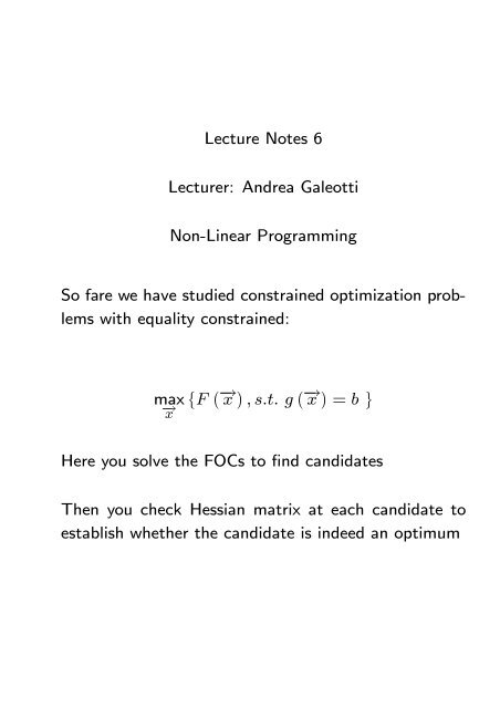
<strong>Lecture</strong> <strong>Notes</strong> 6<br />
<strong>Lecture</strong>r: <strong>Andrea</strong> <strong>Galeotti</strong><br />
<strong>Non</strong>-<strong>Linear</strong> <strong>Programming</strong><br />
So fare we have studied constrained optimization problems<br />
with equality constrained:<br />
max<br />
−→x<br />
© F ¡ −→x ¢ ,s.t. g ¡ −→x ¢ = b ª<br />
Here you solve the FOCs to find candidates<br />
Then you check Hessian matrix at each candidate to<br />
establish whether the candidate is indeed an optimum
Constrained Optimization with Inequality Constraints<br />
s.t. g ¡ −→ x ¢ ≤ b<br />
Two possible solutions:<br />
max<br />
−→x F ¡ −→ x ¢<br />
xi ≥ 0, i =1, ..., n<br />
Solution at which the constraint binds<br />
Solution at which the constraint does not bind
BC<br />
IC<br />
The LHS graph describes a situation were at the optimum<br />
the constraint binds.<br />
The RHS graph describes a situation were at the optimum<br />
the constraint does not bind.<br />
Note that in the RHS there is a point were the BC<br />
and IC are tangent. However, that is not an optimum<br />
becauseyoucouldmovetowardstheoriginanddoing<br />
so the constraint will still hold (will be unbind) and you<br />
will move to a highest indifference curve.<br />
IC<br />
BC
Example:<br />
y 16.25<br />
15<br />
13.75<br />
12.5<br />
11.25<br />
10<br />
0<br />
1.25<br />
2.5<br />
LHS<br />
3.75<br />
x<br />
5<br />
max F<br />
−→<br />
x ≥0 ¡ −→ ¢<br />
x<br />
y<br />
10<br />
8<br />
6<br />
4<br />
2<br />
0<br />
0.5<br />
1<br />
1.5<br />
RHS<br />
LHS: F 0 (x) =0forsomex>0, say x ∗ . This is an<br />
Interior Solution<br />
RHS: F 0 (x) < 0foranyx ≥ 0. The optimum here is<br />
x ∗ =0. This is a corner solution.<br />
2<br />
2.5<br />
x<br />
3
Hence, in the first order conditions for a maximum we<br />
must include both possibilities.<br />
Necessary conditions: −→ x ∗ such that for any i =1,...,n<br />
1) x ∗ i ∂F<br />
∂xi<br />
2) x ∗ i<br />
3) ∂F<br />
∂xi<br />
≥ 0<br />
¡ −→x ∗ ¢ =0<br />
¡ −→x ∗ ¢ ≤ 0<br />
Observe that:<br />
if x ∗ i<br />
is interior: ∂F<br />
∂xi<br />
If x∗ i is a corner Solution, i.e. x∗i satisfied.<br />
How to solve:<br />
¡ −→x ∗ ¢ =0. Thus 1,2,3 are satisfied<br />
= 0. Thus, 1,2,3 are<br />
We guess a solution and then we impose the FOCs<br />
which derive from that solution. This gives us a system.<br />
We solve it and we check that the solution is consistent<br />
with the solution of the first order conditions. In this<br />
case we have a candidate. Otherwise we know that our<br />
guess cannot be an optimum.
Kuhn-Tucker Conditions for Optimality<br />
max F (x)<br />
x<br />
s.t. g (x) ≤ b<br />
x ≥ 0<br />
Define a slack variable s = b − g (x) ≥ 0, then problem<br />
can be rewritten as:<br />
s.t. g (x)+s =<br />
max F (x)<br />
x,s<br />
b<br />
x ≥ 0, s ≥ 0<br />
We define the Lagrangian:<br />
$ (x, s) =F (x)+λ [b − g (x) − s]
Therefore:<br />
Necessary conditions:<br />
(i) conditions for x<br />
x ∂$<br />
∂x<br />
(ii) conditionsfors<br />
s ∂$<br />
∂s<br />
max $ (x, s)<br />
x,s≥0<br />
=0, ∂$<br />
∂x<br />
=0, ∂$<br />
∂s<br />
≤ 0, x ≥ 0<br />
≤ 0, s ≥ 0
Note that (i) isthesameas:<br />
x ∂$<br />
∂x<br />
∂$<br />
∂x<br />
x<br />
=<br />
=<br />
≥<br />
· ¸<br />
∂F<br />
x − λ∂g<br />
∂x ∂x<br />
∂F<br />
− λ∂g ≤ 0<br />
∂x ∂x<br />
0<br />
Note that (ii) isthesameas:<br />
=0<br />
s ∂$<br />
∂s<br />
λ<br />
=<br />
≥<br />
−sλ = −λ [b − g (x)] = 0<br />
0<br />
s = b − g (x) ≥ 0
Thus we have two possibilities:<br />
I) either the constraint does not bind g (x)
We really do not need to bother about the slack variable<br />
s.<br />
We can simply rewriting the original problem as:<br />
And therefore:<br />
FOCs<br />
$ (x, s) =F (x)+λ [b − g (x)]<br />
max<br />
x≥0<br />
x ∂$<br />
∂x<br />
λ ∂$<br />
∂λ<br />
= 0 and λ∂$<br />
∂λ<br />
slackness conditions.<br />
x ∂$<br />
∂x<br />
F (x)+λ [b − g (x)]<br />
∂$<br />
= 0,<br />
∂x<br />
∂$<br />
= 0,<br />
∂λ<br />
≤ 0, x ≥ 0<br />
≥ 0, λ ≥ 0<br />
= 0 are called complementarity
Note: in case of inequality constraints the way in which<br />
the constraint is written matters for the necessary conditions.<br />
To avoid any confusion you should transform each inequality<br />
constraint in the following form:<br />
Thus if the constraint is<br />
function ≤ constant<br />
h (x) ≥ b ⇐⇒ −h (x) ≤−b<br />
And you always write the Lagrangian by inserting the<br />
constraint in the following form:<br />
constant-function
Again, if you must solve:<br />
Then you write as:<br />
And then you write:<br />
s.t. h (x) ≥<br />
max<br />
x≥0<br />
b<br />
s.t. − h (x) ≤<br />
max<br />
x≥<br />
−b<br />
F (x)<br />
F (x)<br />
$ (x) =F (x)+λ [−b + h (x)]
Example:<br />
s.t. px + qy ≤<br />
max U (x, y)<br />
M<br />
x, y ≥ 0<br />
Assume that ∂U/∂x,∂U/∂y > 0. That is an increase<br />
in consumption leads to an increase in utility.<br />
Write the Lagrangian:<br />
$ (x, y, λ; M, p, q) =U (x, y)+λ [M − px − qy]<br />
Necessary conditions<br />
x ∂$<br />
∂x<br />
λ ∂$<br />
∂λ<br />
∂$<br />
= 0,<br />
∂x<br />
∂$<br />
= 0,<br />
∂λ<br />
≤ 0, x ≥ 0<br />
≥ 0, λ ≥ 0<br />
It is easy to see that the constraint should bind at the<br />
candidate, i.e. λ>0.
Indeed note that<br />
∂$<br />
∂x<br />
∂$<br />
∂y<br />
∂U<br />
=<br />
∂x<br />
∂U<br />
=<br />
∂y<br />
− λp =0<br />
− λq =0<br />
Suppose the constraint does not bind. This implies that<br />
λ = 0 and therefore it must be the case that at the<br />
candidate point (x ∗ ,y ∗ )<br />
∂$<br />
∂x<br />
∂$<br />
∂y<br />
= ∂U<br />
∂x (x∗ ,y ∗ ) ≤ 0<br />
= ∂U<br />
∂y (x∗ ,y ∗ ) ≤ 0<br />
which contradicts the fact that U is monotonic in x and<br />
y.
Just to repeat again:<br />
Lagrangian:<br />
Two Constraints<br />
s.t. g1 (x, y) ≤<br />
max F (x, y)<br />
x,y≥0<br />
b1, g2 (x, y) ≤ b2<br />
$ (x, y, λ, µ) = F (x, y)+λ [b1 − g1 (x, y)] +<br />
+µ [b2 − g1 (x, y)]<br />
K.T. Necessary conditions:<br />
(i) conditions for x and y :<br />
x ∂$<br />
∂x<br />
y ∂$<br />
∂y<br />
∂$<br />
= 0; x ≥ 0;<br />
∂x<br />
∂$<br />
= 0; y ≥ 0;<br />
∂y<br />
(ii) conditions for the constraints:<br />
≤ 0<br />
≤ 0<br />
λ [b1 − g1 (x, y)] = 0; λ ≥ 0; g1 (x, y) ≤ b1<br />
µ [b2 − g2 (x, y)] = 0; µ ≥ 0; g2 (x, y) ≤ b2
Suppose the second constraint is a binding constraint<br />
(with equality), i.e. g2 (x, y) =b2.<br />
s.t. g1 (x, y) ≤ b1<br />
g2 (x, y) = b2<br />
max F (x, y)<br />
x,y≥0<br />
In this case µ can take any value because we do not<br />
require it to be strictly or equal to zero. Thus, we<br />
can write this constraint in the Lagrangian function no<br />
matter the way.
Another example: A <strong>Linear</strong> <strong>Programming</strong> Problem:<br />
max U (S, D)<br />
S,D≥0<br />
= 4S + D<br />
s.t. S + D ≤ 10<br />
S +2D ≤ 12<br />
The first inequality constraint represents a time constraint:<br />
An individual has at maximum 10 hours a week to<br />
spend in leisure. Leisure activity can be diversified in<br />
S =sailing and D =diving.
The second inequality constraint is a cash constraint:<br />
The individual has a maximum of 12 pounds a week to<br />
spend in leisure.<br />
S<br />
S+2D=12<br />
S+D=10<br />
What is the combination of sailing and diving which is<br />
feasible and which maximize the utility?<br />
D
First: write the Lagrangian in the right way:<br />
$ (S, D, λ, µ) = 4S + D + λ [10 − S − D]+<br />
+µ [12 − S − 2D]<br />
Second: write down the KT necessary conditions:<br />
S ∂$<br />
∂S<br />
∂$<br />
∂S<br />
D<br />
=<br />
=<br />
S[4 − λ − µ] =0; S ≥ 0;<br />
4−λ− µ ≤ 0<br />
∂$<br />
∂D<br />
∂$<br />
∂D<br />
λ [10 − S − D]<br />
=<br />
=<br />
=<br />
D[1 − λ − 2µ] =0; D ≥ 0;<br />
1−λ− 2µ ≤ 0<br />
0; λ ≥ 0; S + D ≤ 10<br />
µ [12 − S − 2D] = 0; µ ≥ 0; S +2D ≤ 12
Third: Solve by guessing the type of solution.<br />
We know that either there is an interior or a corner<br />
solution<br />
a) Guess an interior solution, i.e. S, D > 0<br />
Thenitmustbethecasethat:<br />
∂$<br />
∂S<br />
∂$<br />
∂D<br />
=<br />
=<br />
4−λ− µ =0<br />
1−λ− 2µ =0<br />
Solving yields to µ = −3, which contradicts the condition<br />
µ ≥ 0.<br />
Thus, the solution should be a corner solution.<br />
Yet, there are many candidates for the corner solution.<br />
We know that one of the two constraints should not<br />
bind.
) Guess that the cash constraint does not bind, i.e.<br />
µ =0<br />
b1) Guess a corner solution S =0andD>0 µ =0,<br />
λ>0<br />
S ∂$<br />
∂S<br />
∂$<br />
∂S<br />
D<br />
=<br />
=<br />
S[4 − λ − µ] =0; S ≥ 0;<br />
4−λ− µ ≤ 0<br />
∂$<br />
∂D<br />
∂$<br />
∂D<br />
λ [10 − S − D]<br />
=<br />
=<br />
=<br />
D[1 − λ − 2µ] =0; D ≥ 0;<br />
1−λ− 2µ ≤ 0<br />
0; λ ≥ 0; S + D ≤ 10<br />
µ [12 − S − 2D] = 0; µ ≥ 0; S +2D ≤ 12
Use your guess:<br />
Violated....<br />
∂$<br />
= 4−λ≤ 0<br />
∂S<br />
D ∂$<br />
= 0 ⇐⇒ λ =1;<br />
∂D<br />
∂$<br />
= 1−λ≤ 0<br />
∂D<br />
D = 10, S +2D ≤ 12
2) Then guess a corner solution: S>0, D=0,µ=0<br />
and λ>0. Then<br />
∂$<br />
∂S<br />
∂$<br />
∂D<br />
λ [10 − S − D]<br />
=<br />
=<br />
=<br />
4−λ =0 ⇐⇒ λ =4<br />
1−λ≤ 0<br />
0 ⇐⇒<br />
10 − S − D = 0 ⇐⇒ S =10<br />
S ≤ 12<br />
Nowyoucanverifythatifyoutake<br />
(S =10,D =0,λ=4,µ=0)<br />
all the K.T. conditions hold.<br />
S<br />
S+2D=12<br />
IC<br />
S+D=10<br />
D
Kuhn-Tucker Sufficiency Theorem<br />
Consider the following programming problem:<br />
s.t. g ¡ −→ x ¢ ≤ b<br />
max F<br />
−→<br />
x ≥0 ¡ −→ ¢<br />
x<br />
After having solve the first order conditions we obtain<br />
a candidate. How do we know that the candidate is a<br />
global maximum?<br />
Theorem: If<br />
(i) F is a concave function<br />
(ii) g isaconvexfunction<br />
(iii) The qualification constraint is satisfied<br />
Then the solution to the K.T. conditions describes a<br />
global maximum.
Note that if the constrained is a linear function, condition<br />
(iii) holds.<br />
In general the qualification constraint is that the Jacobian<br />
matrix of the binding constraints has full rank.<br />
(evaluated at the candidate point.)<br />
Example:<br />
s.t. g (x, y) ≤<br />
max U (x, y)<br />
x,y≥0<br />
b<br />
Suppose U is concave and the constraint is linear. Then<br />
(i) and(ii) and(iii) holds.
Theorem: Arrow-Enthoven Sufficiency Theorem<br />
If<br />
s.t. g ¡ −→ x ¢ ≤ b<br />
(a) F is a quasiconcave function<br />
(b) g is a quasiconvex function<br />
max F<br />
−→<br />
x ≥0 ¡ −→ ¢<br />
x<br />
(c) thequalification constraint is satisfied<br />
(d) ∂F<br />
∂xi 6=0foratleastonei<br />
Then the solution to the K.T. conditions describes a<br />
global maximum.
Take the problem we have analysed before:<br />
Note that:<br />
max U (S, D)<br />
S,D≥0<br />
= 4S + D<br />
s.t. S + D ≤ 10<br />
S +2D ≤ 12<br />
U is concave, so it is quasiconcave<br />
The two constraints are convex, so they are quasiconvex<br />
The qualification constraint is satisfied (the constraints<br />
are both linear)<br />
∂U<br />
∂S =46= 0<br />
So the solution we have found before is a global maximum.
Equivalent to<br />
Now you solve it.<br />
Minimization problem<br />
s.t. F (x) ≥<br />
min C (x)<br />
Q<br />
x ≥ 0<br />
s.t. − F (x) ≤<br />
max −C (x)<br />
−Q<br />
x ≥ 0