SINTEF REPORT

SINTEF Materials and Chemistry 

Address: NO-7465 Trondheim, 

NORWAY 

Location: Brattørkaia 17B, 

4. etg. 

Telephone: +47 4000 3730 

Fax: +47 930 70730 

Enterprise No.: NO 948 007 029 MVA 

TITLE 

SINTEF REPORT 

EIF and deposition calculations for exploration drilling at the 

Pumbaa Exploration Field (PL469). 

Final report 

AUTHOR(S) 

Henrik Rye and May Kristin Ditlevsen 

CLIENT(S) 

Aker Exploration 

REPORT NO. CLASSIFICATION CLIENTS REF. 

SINTEF A11340 Unrestricted Morten Løkken 

CLASS. THIS PAGE ISBN PROJECT NO. NO. OF PAGES/APPENDICES 

Unrestricted 978-82-14-04761-5 801195.13 47 

ELECTRONIC FILE CODE PROJECT MANAGER (NAME, SIGN.) CHECKED BY (NAME, SIGN.) 

Final report PL469 EIF.doc Henrik Rye Mark Reed 

FILE CODE DATE APPROVED BY (NAME, POSITION, SIGN.) 

ABSTRACT 

23 March 2009 Tore Aunaas, Research Director 

An exploration drilling is planned on the Pumbaa field (PL 469) in the Norwegian Sea. This report 

shows the results from calculation of the potential environmental risks (and the associated EIF values) 

for the water column and the sediment caused by the planned drilling operations. Exposure calculations 

for some typical coral locations are also performed. 

All calculations are carried out with the DREAM model version 4.0 operated by SINTEF. 

KEYWORDS ENGLISH NORWEGIAN 

GROUP 1 Environment Miljø 

GROUP 2 Discharge to sea Utslipp til sjø 

SELECTED BY AUTHOR Numerical modelling Numerisk modellering 

Drill cuttings and drilling fluid Borekaks og boreslam 

Risk estimates Risikovurderinger

SUMMARY: 

An exploration drilling is planned on the Pumbaa field (PL 469) in the Norwegian Sea. The 

present report shows the results from calculation of the potential environmental risks (and the 

associated EIF values) for the water column and the sediment caused by the planned drilling 

operations. Potential impacts on corals located nearby are addressed in particular. 

The well comprises 6 sections, drilled with Water Based Mud (WBM). 4 sections (42”, 9 7/8” 

pilot hole, 36” and 26”) give discharges directly to the sea floor, while two sections (17 ½” and 

12 ¼”) give discharges from the drilling rig. 

EIF results 

The results from the EIF calculations are summarized in the table below: 

Summary of results from EIF calculations. 

Scenario Compartment Max. Duration for Dominant risk 

impacted EIF EIF > 0 contributor 

Base case Upper water 

column 

2255 4 days Barite part. 

Lower water 

157 6 days Bentonite and barite 

column 

part. 

Sediment 58 > 10 years Copper in barite 

The results show that for the water column, particle effects caused by discharges of particle matter 

(barite and bentonite) are dominating the risk for both the upper and lower water column. The 

particles may impact on organisms that are filtering sea water (like sea shells, scallops, 

zooplankton, fish). For the sediment, heavy metals in the particle matter represent the largest 

potential for environmental risk. The presence of heavy metals in barite and bentonite that deposit 

on the sea floor will partly dissolve in the sediment pore water, and thus become bioavailable. Cu 

in barite gives the largest risk contribution, caused by a relatively large concentration of Cu in the 

barite that is planned to be used. Later results indicate that the risks associated with Cu in barite 

are probably over-estimated. 

The values of the EIF’s are largest for the water column impact. However, the duration period of 

impact is significantly shorter than for the duration of impact for the sediment. When the EIF’s 

are adjusted according to duration of impact, the revised EIF (denoted EIFyear) becomes of order 

300 – 500 for the sediment (adjusted for a 10-year duration of impact), and of order 3 - 30 for the 

water column (durations about 4 - 6 days for the water column impacts). Although the impacts in 

the sediment and in the water column are not directly comparable, the order-of-magnitude 

differences of the EIFyear’s for the water column and sediment indicate that the potential sediment 

impact may be judged to be more severe that the potential water column impact (due to its short 

duration) 1 . Therefore, the heavy metal content in barite appears to represent the largest potential 

for environmental impact for the present EIF simulation. 

1 

One of the basis for the intercomparison between water column and sediment EIF’ s are that both EIF’s are based on 

a unity on the horizontal scale equal to 100m x 100m. 

I:\prosjekt\8016-Marin_miljoteknologi\MK801195_Geitefjellet_eksploration_drilling_HR\Adm\Notater_Rapporter\Final_Report PL469 EIF.doc 

2

Impact on corals 

Corals are present in the area where the drilling operations are planned. Two types of impacts can 

be envisaged: 

• Impacts caused by burial 

• Impact on on corals through filtering behavior 

Impacts caused by burial are described in Chapter 5.1. Criteria for damage expected on corals 

caused by drilling discharges are not established. In the present report, results are shown for 

depositions that exceed the expected natural deposition in the area on a yearly basis. In the 

recently published report on ”Consequences caused by regular discharges to sea, Norwegian Sea 

area” 2 , an estimate of the natural sedimentation rate in this area (over-all values) is presented. 

Based on observations of existing natural depositions in the area, of order 0.01 – 0.02 mm/year 

was arrived at. Therefore, results are shown for added depositions caused by the drilling 

discharges down to 0.01 mm in total. The simulations carried out show that this amount of burial 

caused by the discharges should be expected up to order 800 – 900 m from the well location in 

direction N – S, and up to 2 km from the well in the E – W direction. These distances include the 

location of some corals in the vicinity of the well. 

Impacts on corals through filtering are described in Chapter 5.2. The potential for impact can be 

illustrated by showing time series of total particle content in the water masses close to the sea 

floor. The corals are feeding on (or filtering) particle matter present in the water column. The 

corals may therefore also be impacted by particles suspended in the water masses before they 

settle on the sea floor. These particles comprise essentially the finer fractions of the particles 

originating from the top hole section discharges. Because some coral locations are relatively close 

to the planned well, some suspended matter may pass the coral locations when the current 

direction coincides with the direction of coral location from the well. 

The period of impact will be restricted to the period of discharge from the top hole sections, 

essentially (neglecting the possibility of re-suspension of the deposited matter). Time series of 

calculated concentration of particle matter shows that some of the coral locations closest to the 

drilling site may occasionally experience exceedence of potential no-effect concentrations 

(PNEC’s) for barite and bentonite particle concentrations in the water column. This exposure will 

be very occasionally, restricted to the periods when the direction of the currents coincides with the 

direction of the location of the corals. When the directions coincide, the particle concentrations in 

the plume generated tend to exceed the PNEC levels of the particle matter for the coral locations 

closest to the drilling site (order 200 - 300 m from the well). Therefore, it may be a potential for 

environmental impact on the corals, but it should be noted that the time duration of the impact is 

rather small (order some hours, at maximum, for each time the plume hits the corals during 

discharge). For the 800 m location, the concentrations during the hit are expected to be smaller 

(below 0.3 ppm). This value is close to the PNEC values for the particle matter. The reduction in 

the concentration level is partly due to dilution of the discharge “cloud” at the sea floor and also 

partly due to that some of the content in the “cloud” is depositing on the sea floor while the 

“cloud” moves with the currents along the sea floor. 

2 SINTEF: Konsekvenser av regulære utslipp til sjø. Helhetlig forvaltningsplan for Norskehavet (HFNH). Program 

for utredning av konsekvenser. Sektor Petroleum og Energi. Report made for DNV/OED dated 26 February 2008. 

SINTEF report SINTEF F5543. SINTEF project No. 800923. 


3

ABBREVIATIONS 

BOP Blow-Out Preventer 

CB Background concentration of metal in sediment 

DREAM Dose related Risk and Effect Assessment Model 

EC50 The concentration where a specific effect is observed for 50% of the test 

specimen 

EIF Environmental Impact Factor 

ERMS Environment Risk Management System 

HOCNF Harmonized Offshore Chemical Notification Format 

KOC Partition coefficient organic carbon - water 

LC50 The concentration which causes lethality for 50% of the test specimen 

LOEC Lowest Observed Effect Concentration 

MEMW Marine Environmental Modelling Workbench 

MPA Maximum Permissible Addition 

MPC Maximum Permissible Concentration 

NCS Norwegian Continental Shelf 

NOEC No Observed Effect Concentration 

OBM Oil Based Mud 

OLF The Norwegian Oil Industry Association 

PAH Poly-Aromatic Hydrocarbons 

PEC Predicted Environmental Concentration/Change 

PNEC Predicted No Effect Concentration/Change 

PLONOR Pose Little or No Risk to the environment 

POW Partition coefficient used in the HOCNF testing of offshore chemicals 

SBM Synthetic Based Mud 

SFT Norwegian State Pollution Control Authority 

SPM Suspended Particle Matter 

SSD Species Sensitive Distributions 

TGD Technical Guideline Document (EC 1996) 

THC Total HydroCarbons in sediment 

WBM Water Based Mud 


4

Table of Contents Page 

1 Introduction............................................................................................................................6 

2 The DREAM model and the EIF concept............................................................................7 

2.1 The DREAM model ..........................................................................................................7 

2.2 The EIF concept in general .............................................................................................12 

2.3 Special features for the EIF drill cuttings and mud discharges.......................................16 

3 Input data .............................................................................................................................19 

3.1 General ............................................................................................................................19 

3.2 Location...........................................................................................................................20 

3.3 Particle size of the natural sediment................................................................................21 

3.4 Grain size distributions in the discharge .........................................................................21 

3.5 PNEC’s for particles and components in the mud packages used. .................................23 

3.6 PNEC’s for heavy metals in sediment.............................................................................23 

3.7 Time duration of the discharges......................................................................................24 

3.8 Discharge configurations................................................. Error! Bookmark not defined. 

3.9 Summer heating stratification .........................................................................................25 

3.10 Ambient winds and currents conditions .........................................................................25 

3.11 Discharge setup for the various drilling sections ...........................................................26 

3.12 Presence of corals...........................................................................................................28 

4 EIF Results ...........................................................................................................................30 

4.1 General ............................................................................................................................30 

4.2 EIF Results for the upper water column..........................................................................31 

4.3 EIF Results for the lower water column..........................................................................33 

4.4 EIF Results for the sediment. ..........................................................................................35 

4.5 Summary of EIF results and discussion. .........................................................................37 

5 Impact on corals...................................................................................................................39 

5.1 Results from calculation of potential coral impact caused by deposition.......................39 

5.2 Results from calculation of potential coral impact caused by particle content in the water 

column.............................................................................................................................44 

References ....................................................................................................................................46 


5

1 Introduction 

An exploration drilling is planned on the Pumbaa field (PL469) in the Norwegian Sea. The 

present report shows the results from calculation of the potential environmental risks (and the 

associated EIF values) for the water column and the sediment caused by the planned drilling 

operations. The well comprises 6 sections, drilled with Water Based Mud (WBM). 4 sections 

(42”, 9 7/8” pilot hole, 36” and 26”) give discharges directly to the sea floor, while two sections 

(17 ½” and 12 ¼”) give discharges from the drilling rig. 

The present report contains the results from the discharge fates and corresponding risk 

calculations. The calculations are carried out with the revised DREAM model, version 4.0. 

The present report comprises the following chapters: 

• Description of the DREAM model and the EIF concept (Chapter 2) 

• Details of model input data. Drilling location and drilling sections. Size distributions of 

particle matter. Heavy metal content. The mud package composition for each section. 

Also, ambient conditions (currents and ambient stratification) are described. Presence of 

corals (Chapter 3). 

• Modelling with the DREAM model discharges and fates, incuding EIF results for both the 

water column and sediment. Presentation and discussion of results (Chapter 4). 

• Results of the DREAM calculations with respect to potential impacts on corals. Results for 

the water column close to sea floor (lower water column). Depositions on the sea floor. 

Interaction with corals present in the area. Presentation and discussion of results (Chapter 

5). 

• References are included after Chapter 5. 

The model versions used in the present study are denoted MEMW 4.0.5 dated 21. August 2008 

(Fates.exe) and 03. October 2008 (MEMW.exe). The module for presentation graphics 

(MEMW.xls) is dated 27 September 2007. 


6

2 The DREAM model and the EIF concept 

2.1 The DREAM model 

The following description of the DREAM model is taken from Rye et. al (2008): 

The numerical model approach is based on the DREAM model, as it has been applied to produced 

water risk assessments (Johnsen et al. 2000). In addition, some modules of the numerical model 

ParTrack for calculation of dispersion and deposition of drill cuttings and mud (Rye et al. 1998, 

2004; 2006) have been implemented. The model concept applied is a “particle”, or Lagrangian 

approach. The model generates particles at the discharge point, which are transported with the 

currents and turbulence in the sea. Different properties, such as the mass of various compounds, 

densities and sinking velocities, are associated with each particle. Model particles can also 

represent different states or phases, such as bubbles, droplets, dissolved matter and solid matter. 

For discharges of drill cuttings and mud, solid particles, organic matter, metals attached to solid 

particles and dissolved matter will be of particular interest. The formulas applied for spreading in 

the water column are given in Reed and Hetland (2002). 

The ocean current field applied in the DREAM model is usually imported from outputs generated 

from 3-dimensional and time-variable hydrodynamic models. It is also possible to apply observed 

ocean current profiles generated from measurements at a specific location. 

Generic features for the calculation of deposition. A more reliable description of the behavior of 

drilling discharges has been undertaken by incorporation of additional modules into the model 

system. These include a near field plume, sinking velocities of particles depositing on the sea 

floor and particle size distributions specified for each particle group (cuttings, barite). 

Near-field plume. Discharges of drill cuttings and mud have densities that are significantly higher 

than the ambient water. A near field plume is therefore included in order to account for the 

descent of the plume. This descent will cease when the density of the descending plume equals the 

density of the ambient water. The plume path is governed by the ocean current velocities (and 

directions) and also by the vertical variation of the ambient salinity and temperature 

(stratification). The combination of these factors causes the plume to level out at some depth (the 

“depth of trapping”) or sink down to the sea floor and level out there. Mineral particles (cuttings, 

weight material) are allowed to fall out of the plume, dependent on the sinking velocity and the 

rate of entrainment of water into the plume. The principal features of the near field plume model 

are given in Johansen (2000, 2006). 

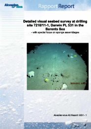
Descent of particles to the sea floor. Figure 2.1 shows a vertical cross section of an underwater 

plume on the downstream side of the release site calculated with the DREAM model. The “depth 

of trapping” in the case shown indicates that this appears at about 20 m depth (discharge depth is 

about 5 m). At this depth, the underwater plume separates into 2 parts: 1) To spread horizontally 

at the depth of trapping. This part consists of dissolved compounds (not sinking) and of solid 

particles that are so small in diameter that sinking velocities are negligible. 2) The other part of 

the discharge appears to sink down to the sea floor. This part may consist of coarser particles (like 

cuttings particles with relatively large diameters) with some chemicals attached to them. 


7

Figure 2.1 An example illustrating the vertical cross section of the near field plume and the 

deposition of particles on the sea floor. Discharge point to the upper left corner of 

the figure. Sea floor at about 400 m depth. 

The sinking velocities of the particles can be divided into 2 regimes, the Stokes regime and the 

Constant drag regime. The sinking velocities within the Stokes regime for smaller particles are 

given by Equation 1: 

2 

d g' 

W 1 = 

18υ 

(1) 

where W1 is laminar Stokes sinking velocity of a particle, d is the particle diameter, g’ is the 

reduced gravity = g ( ρ particle − ρ water ) / ρ water , g is the standard gravity, ρ is the density of particle 

or sea water and υ = kinematic viscosity = 1.358 x 10 -6 m 2 /s at 10 o C for sea water. 

The second contribution to the sinking of the particles is the friction dominated Constant drag 

regime for larger particles. A general expression for this sinking velocity can be derived from the 

balance between buoyancy forces and drag forces acting on the particle (Hu and Kintner, 1955) 

calculated by Equation 2: 

W 

4 d g' 

3 

2 = (2) 

CD 


8

The drag coefficient CD in this equation is a function of the Reynolds number ( Re 2 / ν d W = ). On 

this basis, two asymptotic regimes are identified, the Stokes regime and the Constant drag regime 

(Equation 3): 

1) Stokes regime (Re 

< 1) : 

2) Constant drag regime (Re 

2 

d g' 

W1 

= 

18ν 

(3) 

> 1000) : W = K d g' 

2 

where K is an empirical dimensionless constant. For intermediate values of the Reynolds number 

(1 < Re < 1000), an interpolation equation for the total sinking velocity W of the particle may be 

used, expressed by the Equation 4: 

W = 

⎛ 1 

⎜ 

⎝W 

1 

1 

1 ⎞ 

+ ⎟ 

W2 

⎠ 

The empirical constant K is chosen so that correspondence is reached between the friction 

dominated sinking velocity as given in US Army Coastal Engineering Manual (2007) and the 

Equation 3 above. This equation takes into account that grains are usually non-spherical and have 

therefore generally lower sinking velocities than grains with spherical shapes. 

A graphical presentation of the curve shape given by Equation 4 is shown in Figure 2.2. For low 

diameter particles (diameters lower than 2 x 10 -4 m), the equation corresponds well with the 

Stokes sinking velocity (Equation 1). For larger particle diameters (diameters larger than 2 x 10 -3 

m), the equation corresponds well with the friction dominated velocity (Equation 2). In the 

diameter range in between, the sinking velocities are influenced by contributions from both 

regimes. 

Deposition of chemicals on the sea floor--In WBM (Water based Mud), most of the added 

chemicals are mainly assumed to dissolve in the water column. For other types of mud (e.g. OBM 

and SBM, Oil Based Mud and Synthetic Based Mud), dissolution of the chemicals in the water 

column may be slow. These chemicals (typically exhibiting large octanol – water partition 

coefficient Kow) may also have a high capacity for adsorption to organic matter present in the 

sediment or water column. 


(4) 

9

Rise velocity, m/s 

Sinking velocity, m/s 

1.0E+00 

1.0E-01 

1.0E-02 

1.0E-03 

1.0E-04 

Stokes law 

Constant drag 

1.0E-05 

1.0E-05 1.0E-04 1.0E-03 1.0E-02 

Particle diameter, m 

Figure 2.2 Particle size dependent variation in fall velocity of mineral particles in seawater. 

Solid density 2500 kg/m 3 , resembling cuttings particles. Thin lines: Stokes law and 

constant drag law. Thick line: Interpolation formula. 

According to the EC (2003), substances with Koc < 500 – 1000 L/kg are not likely to adsorb to 

sediment. The EC (2003) states that “To avoid extensive testing of chemicals, a logKoc or logKow 

of ≥ 3 (or ≥ 1000 L/kg) can be used as a trigger value for sediment effects assessment”. 

In accordance to the TGD the chemicals with low Kow or Koc values (< 1,000 L/kg) are assumed 

to dissolve (completely) in the water column. For large Kow or Koc values ( ≥ 1,000 L/kg), the 

chemicals are assumed to adsorb (or “attach”) to particles and eventually deposit on the sea floor. 

This process may take place either through “agglomeration” (in which new particles are formed), 

or by “attachment”, where chemicals are thought to “attach” to individual mineral particles in the 

discharge. The Kow and Koc are partition coefficients, the Kow is the octanol-water partition 

coefficient, and the Koc is the particle organic carbon partition coefficient. The relationship 

between Koc and Kow has been studied by Di Toro et al. (1991). It was found that Koc and Kow are 

closely related. The TGD (EC 2003) does not differentiate between use of Kow or Koc. Therefore, 

it is recommended to use Kow if no Koc value is available for organic substances. The octanolwater 

partition coefficient denoted Pow is assumed equal to Kow. 


10

Figure 2.3 shows the basic features of the developed model for calculating the fate of drilling 

discharges. Concentrations in the water column and depositions on the sea floor are illustrated. 

The particles in the model have been spread in the recipient due to ocean currents and turbulence 

(after the termination of the near field plume phase). 

Ecological risks in 

water column 

and sediments 

Vertical cross section 

Water column 

concentrations Sediment 

concentrations 

and stressors 

Complete 

mass 

balance 

Time (days:hrs:min) 

Figure 2.3 Visualization of the fate of drilling discharges. The figure demonstrates the 

following: 

1). Concentrations of dissolved compounds (and/or particle matter) calculated for the 

water column, concentrations shown in ppm (mg/L). 

2). Deposition of the particle matter on the sea floor (along with chemicals attached 

to the particles), deposition in kg/m 2 sediment surface. 

3). A mass balance histogram that shows the amounts that are depositing on the sea 

floor, and the amounts that remain in the water column. 

4). A vertical cross section that shows the plume in the water column (close to sea 

surface) and the deposition of particles falling out below the plume. The actual cross 

section chosen is shown by an arrow on the main figure. 


11

2.2 The EIF concept in general 

General. The operators on the Norwegian Continental Shelf (NCS) have agreed with the 

Norwegian Authorities to work towards a reduction of the environmental impacts from produced 

water releases (and from drill cuttings and mud releases as well) down to a level of “zero harmful 

effects”. To more clearly define this goal, the EIF (Environmental Impact Factor) has been 

developed as an indicator of the environmental risk caused by regular releases to sea. The EIF is 

used as a measure of the environmental benefit achieved when alternate measures are considered 

for reducing environmental impacts. 

The method has the advantage that it gives a quantitative measure of the environmental risks 

involved when effluents are discharged to sea, and is thus able to form a basis for reduction of 

impacts in a systematic and a quantitative manner. 

This method is based on the calculation of the EIF using the numerical model DREAM (Dose 

related Risk and Effect Assessment Model) developed by SINTEF, with financial support from 

StatoilHydro, ENI, Total, ExxonMobil, Petrobras, ConocoPhillips, and Shell. 

General description of the method. The EIF method is based on a PEC/PNEC approach, in which 

the concentration for each compound discharged into the recipient is compared to a concentration 

threshold for that compound. When the predicted (modeled) environmental concentration (PEC) is 

larger than the predicted no-effect concentration (PNEC), an “unacceptable” environmental risk 

for damage is encountered. When the PEC is lower than the PNEC threshold, the environmental 

risk is considered to be “acceptable”. 

An outline of the EIF method applied to produced water discharges is given in Johnsen et. al., 

2000. 

The PEC. The PEC (Predicted Environmental Concentration) is the three-dimensional and time 

variable concentration in the recipient caused by the discharge to sea. The PEC is calculated for 

all compounds in the discharge that are assumed to represent a potential for harmful impact on the 

biota. The calculations are carried out by using the numerical DREAM model. This model is fully 

three-dimensional and time variable. It calculates the fate in the recipient of each compound 

considered under the influence of 

• currents (tidal, residual, meteorological forcing) 

• turbulent mixing (horizontal and vertical) 

• evaporation at the sea surface 

• reduction of concentration due to biodegradation 

The PNEC. The PNEC (Predicted No Effect Concentration) is the estimated lower limit for 

effects on the biota in the recipient for a single chemical component or component group. A 

PNEC level is given for each component present in the discharge. It is derived from laboratory 

testing of toxicity for each component (or chemical product) in question. The PNEC value is 

derived from EC50, LC50 or NOEC values from laboratory testing, where the EC50, LC50 or the 

NOEC value determined is divided by some assessment factor in order to arrive at the expected 

PNEC. 

A major data collection work has been performed in order to obtain data of sufficient reliability to 

be selected for determination of PNEC values. Different procedures have been selected for 

determination of the PNEC values for added chemicals in drilling mud (and produced water as 


12

well). The PNEC values for added chemicals can be derived from information found in the 

HOCNF (Harmonized Offshore Chemical Notification Format) scheme. Further details can be 

found in Johnsen et. al., 2000 (produced water case). 

Environmental risk and the EIF. The EIF for a single component or component group is related to 

the recipient water volume where the ratio PEC/PNEC exceeds unity. The ratio PEC/PNEC is 

related to the probability of exceedence of the PNEC level according to a method developed by 

Karman et. al., 1994 (and also published in Karman and Reerink, 1997). When PEC/PNEC = 1, 

this corresponds to a level at which there exists a risk for impact to the 5% most sensitive species. 

Figure 2.4 shows the relation between the PEC/PNEC ratio and the probability of environmental 

impact. 

The EIF method has the advantage over other risk assessment methods in that it can calculate risk 

contributions from a sum of chemicals and/or natural compounds in the recipient. For the total 

risk from a sum of compounds, the total risk is calculated formulas for the sum of independent 

probabilities: 

P( A + B) 

= P( 

A) 

+ P( 

B) 

− P( 

A) 

* P( 

B) 

(5) 

where P(A) is the probability of environmental risk for compound A and P(B) is the probability of 

risk for compound B. For small risks (that is, P(A) and P(B) are both small), or risks from 

chemicals which are toxicologically similar in their activity, the risks can be considered to be 

linearly additive, approximately. The method does not account for interactions among chemicals. 

Probability of 

environmental injury (%) 

100 

80 

60 

40 

20 

0 

PEC/PNEC ratio versus environmental risk 

5% ~ PEC/PNEC = 1 

0.01 0.1 1 10 100 1000 10000 

Ratio PEC/PNEC 

Figure 2.4 Relation between the PEC/PNEC level and the risk level (in %) for impact to biota. 

Based on Karman et. al., 1994. PEC/PNEC = 1 corresponds to a level at which 

there exists a possibility of impact to the 5% most sensitive species. 


13

The total risk resulting from all components in a release is calculated by the DREAM model in 

space and time within the model domain. The sum of risks (for every point in space and for each 

time) is then summarized and converted back to a nominal PEC/PNEC value with the aid of the 

function in Figure 2.4. The results are then presented as shown in Figure 2.5 (snapshot in time). 

Results can also be presented as risk in percent. The water volume indicated by red then indicates 

the water volume where the nominal PEC/PNEC is larger than one. Note that the PEC/PNEC 

ratios for all individual components in the release may be less than unity, but the cumulative risk 

from all components may exceed 5%, such that the nominal PEC/PNEC ratio produced by the 

procedure described above, and representing a conglomerate value for the release, exceeds unity. 

56°34'N 

56°32'N 

56°30'N 

2 km 

3°10'E 

3°10'E 

3°15'E 

3°15'E 

Risk Map Time Series 

Figure 2.5 Calculation of PEC/PNEC for the sum of various compounds in a discharge. 

Snapshot in time. Horizontal extent (upper figure) and vertical extent (lower figure) 

are both shown. 


8:12:00 

56°34'N 

56°32'N 

56°30'N 

14

An EIF of unity is defined as a water volume 100m x 100m x 10m (10 5 m 3 ) in which there is a 

risk of impact to the 5% most sensitive species. For a single component, this corresponds to a 

PEC/PNEC ratio exceeding unity. In addition, the EIF water volume is adjusted upwards by a 

factor of two for those compounds that have a small biodegradation factor combined with a large 

bioaccumulation factor (sometimes called “red” chemicals). Details are given in Johnsen et al., 

2000. 

An attractive feature of the EIF approach is that the method is able to discriminate among the 

various contributors to environmental risk. An example of the distribution of contribution to risk 

among components in a release is shown in Figure 2.6. This capability provides useful 

information when comparing alternative proposed methodologies for reducing environmental 

risks associated with a discharge. 

Thus it is possible to separate a chemical product into its constituents and calculate the EIF 

contribution from each of them. The results of the calculations can then be used to improve the 

product in terms of replacing the constituents in the product with the largest contribution to the 

EIF. 

Total risk, EIF = 0.2678 

Corrosioninhibitor 

0 % 

Corrosioninhibitor 

0 % 

Zi 

0 % 

Ni 

0 % 

BTEX 

1 % 

Naphthalenes 

0 % 

De-emulgation 

chemical 

2-3 ring PAH 

1 % 

0 % 

4-ring+ PAH 

18 % 

Scale inhibitor 

47 % 

Aliphatics 

9 % 

C4+ phenol 

12 % 

Phenol C0-C3 

12 % 

Figure 2.6 Distribution of contribution to risk for an EIF calculation. Here the scale inhibitor 

contributes 47 % of the total risk. 


15

2.3 Special features for the EIF drill cuttings and mud discharges 

EIF for drilling discharges for the water column is defined similarly as for produced water 

discharges. EIF for toxic compounds in the drilling mud is therefore calculated is the same way as 

outlined above for the water column. In addition, risks caused by particle stress on filtering 

organisms in the water column (typically caused by barite and bentonite particles) are included as 

well. 

The risks for discharges of drill cuttings and mud include more stressors than for produced water 

(6 stressors instead of 1, two for the water column and 4 for the sediment). Figure 2.7 illustrates 

how the various compounds in a drilling discharge impacts on the various stressors in the water 

column and in the sediment: 

Impact on water column: 

Discharge compound: Impact: 

Chemicals with Pow < 1000 

Chemicals with Pow ≥ 1000 

Heavy metals in barite 

Particles in mud 

Cuttings 

Impact on sediment: 

Discharge compound: Impact: 

Chemicals with Pow < 1000 

Chemicals with Pow ≥ 1000 

Heavy metals in barite 

Particles in mud 

Cuttings 

Chemical stress 

Particle stress 

Water column 

Sediment 

Water column 

Sediment 

Chemical stress 

Oxygen depletion 

Grain size change 

and burial 

Figure 2.7 Illustration of the impact calculated for the water column (upper figure) and for the 

sediment (lower figure) caused by the various ingredients in the drilling discharges. 


16

Another feature that is different from the produced water is the time variability of the discharges. 

The discharges from a drilling rig to the sea are rather intermittent and time variable, with various 

composition and amounts of the mud discharged from each drilling section. This causes 

corresponding time variability in the EIF. This is expressed in terms of presenting the EIF as a 

time function, with the corresponding risk contributions shown as a function of time as well. An 

example of presenting the EIF for such a case for the water column is shown in Figure 2.8. 

g 

EIF 

300 

250 

200 

150 

100 

50 

0 

0.0 

0.4 

0.9 

1.3 

1.8 

2.2 

2.6 

3.1 

3.5 

3.9 

4.4 

4.8 

Time development chart 

5.3 

5.7 

Time (days) 

Figure 2.8 Time series development of the EIF for the water column caused by drilling 

discharges. Impacts are intermittent according to the discharges from the different 

drilling sections. The main contribution comes from barite and a chemical for the 

case shown. The duration of the impact is limited to between day 3 and 7, basically, 

for the case shown. Unit for the EIF in the water column is a water volume equal to 

100m x 100m x 10m. 


6.1 

6.6 

DAYS 

7.0 

7.4 

7.9 

24.0 

586.4 

1216.4 

1846.4 

2476.4 

3106.4 

EIF_Ilmenite 

EIF_Bentonite 

EIF_Barite 

EIF_Cuttings 

Defoam-AL-comp4 




Ultrafree NS 

Safe-Scav HS 

Safe-cide 

EIF_MEG 

Ultracap 

EMI-939 

EIF_Lead_Bentonite 

EIF_Mercury_Bentonite 

EIF_Cadmium_Bentonite 

EIF_Mercury_Ilmenite 

EIF_Chromium_Ilmenite 

EIF_Lead_Barite 

EIF_Mercury_Barite 

EIF_Copper_Barite 

EIF_Cadmium_Barite 

Defoam-NS 

OCR 325 AG 

Bestolife 3010 NM 

17

Likewise, for the impact on the sediment, the impact may be intermittent and time variable as 

well. A special feature here is that the time of the impact may extend far beyond the duration of 

the discharge. As an example, if biodegradable chemicals (with large Pow partition coefficients) 

attached to cuttings are depositing on the sea floor along with the cuttings particles, the 

biodegradation of the chemicals may consume oxygen from the sediment layers and thus cause 

anoxic conditions in the sediment. Such a case is shown by an example in Figure 2.9. 

A separate “sediment module” that calculates the fate of the particles deposited and chemicals in 

the sediment is also developed. This module calculates the effects from bioturbation (mixing in 

the sediment layer due to the presence of biota), oxygen consumption and partition of chemicals 

between sediment and pore water compartments. Equilibrium partition principle is used. The 

matter dissolved in the pore water is assumed to be bioavailable. Both chemicals and heavy metals 

attached to particle matter are assumed to dissolve in the pore water. Restitution of the sediment 

layer due to biodegradation of chemicals and mixing caused by bioturbation are included as well. 

EIF 

14 

12 

10 

8 

6 

4 

2 

0 

0.0 

0.2 

Grain size 

Oxygen 

Thickness 

Drill-chem-4 

Drill-chem-1 

LUBR-1 

EIF_Zinc_Barite 




EIF_Chromium_Barite 


0.4 

0.6 

0.8 

0.9 

1.1 

1.3 

1.5 

1.7 

1.9 

2.1 


2.3 

2.4 

2.6 

2.8 

3.0 

3.2 

Time (days) 

DAYS 

Figure 2.9 The time development of the EIF for the sediment caused by drilling discharges. 

Note that although the discharge is lasting for some days only, the impact on the 

sediment layer is extending over a time period of more than 10 years. The oxygen 

depletion (yellow contribution) is lasting of order one year before the 

biodegradable chemicals have been biodegraded. Other significant contributions to 

the sediment stress are change of grain size (introduction of “exotic” sediment) and 

burial (denoted “thickness” in the legend). In addition, heavy metals present in 

barite (Cu in particular) contribute to toxicity in the sediment. Unit of the EIF for 

the sediment is 100m x 100m sediment surface. 


3.4 

3.6 

3.8 

3.9 

4.1 

4.3 

4.5 

4.7 

4.9 

5.9 

572.8 

1382.8 

2192.8 

3002.8 

18

3 Input data 

3.1 General 

As illustrated in Figure 2.7, the risks associated with discharges of drill cuttings and mud to sea 

are related to impacts both in the water column and the sediment. The calculation of 

environmental risks for the water column includes two types of “stressors”: 

• Dissolved non-PLONOR compounds or chemicals. These are calculated as dissolved 

chemicals in the water column. Only compounds with a logPow < 3 are included, because 

these are assumed to dissolve in the water column and thus appear in a bioavailable form. 

Compounds with a log Pow ≥ 3 are assumed to “attach” to particles, sink down with the 

particles and thus enter the sediment layer on the sea floor. Here they may contribute to 

environmental risks in the sediment (see below). 

• Particle stress from barite or other types of particles present in the water column. 

For the sediment layer, four stresses are calculated: 

• Toxicity caused by chemicals in the sediment layer. Only compounds with a logPow ≥ 3 

are included. These are assumed not to dissolve in the water column, but attach to particles 

and enter the sediment layer. Here they will biodegrade and therefore contribute to oxygen 

depletion in the sediment layer. Stresses in the sediment caused by heavy metals in particle 

matter are included as well. These may cause toxicity in the sediment but does not 

contribute to oxygen consumption. 

• Excessive oxygen consumption in the sediment layer due to biodegradation of organic 

chemicals. 

• Thickness of deposited matter due to deposition of particle matter on the sea floor. 

• Stresses originating from change of grain size in the sediment layer caused by the particle 

depositions. 

In order to calculate these stressors, a variety of input information must be made available. This 

chapter describes the information that has been applied as input to the DREAM calculations in the 

Pumbaa exploration drilling case (PL469). 


19

3.2 Location 

The co-ordinates of the Pumbaa exploration drilling case (PL469) are 64° 09’ 40.44” N 7° 48’ 

27.87” E. The water depth is 307 meter. A map of the location is shown in Figure 3.1. 

Figure 3.1 Location of the Pumbaa exploration drilling well (PL469). 


20

3.3 Particle size of the natural sediment 

The model calculates the stresses caused by the deposition of grains that have sizes that are 

different from the natural grain sizes on the actual location. Therefore, the actual natural grain size 

on the location should be known. 

However, no surveillance has (so far) been carried out at the actual location. The natural grain size 

at the location is therefore not known. Therefore, the natural grain size has been judged to be 

about 0.1 mm based on information found in ERMS project report No 12 (available at: 

http://www.sintef.no/Projectweb/ERMS/ ). This report shows median particle sizes of natural 

sediment as a function of water depth on the Norwegian Continental Shelf. But the results related 

to natural grain size changes should be considered as rather uncertain due to lack of field data 

from the actual location. 

3.4 Grain size distributions in the discharge 

The discharges consist to a large extent of particles (cuttings, barite and bentonite). Cementing 

discharges are neglected. The grain size of cuttings particles have been investigated by Saga 

(1994). A typical distribution found by them is given in Table 3.1. 

Table 3.1 Grain size distributions of cuttings particles measured during an exploration 

drilling in the Barents Sea. From Saga (1994). Density of cuttings 2500 kg/m 3 . 

DRILL CUTTINGS 

Diameter Weight Density Velocity Velocity 

mm % SG m/s m/day 

0.007 10 2.5 1.9E-05 1.7 

0.015 10 2.5 8.8E-05 7.6 

0.025 10 2.5 2.5E-04 21.2 

0.035 10 2.5 4.8E-04 41.6 

0.05 10 2.5 9.8E-04 84.9 

0.075 10 2.5 2.2E-03 191.0 

0.2 10 2.5 1.6E-02 1356.5 

0.6 10 2.5 5.7E-02 4898.9 

3 10 2.5 2.1E-01 17988.5 

7 10 2.5 3.2E-01 27483.8 


21

Other particle ingredients in the discharge include barite as the weight material. A particle size 

distribution found by Saga (1994) for barite particles is shown in Table 3.2. 

Table 3.2 Grain size distributions of barite particles measured during an exploration drilling 

in the Barents Sea (Saga 1994). The sampling of the barite is taken at the shaker, 

after the particles have been through the drill pit. 

BARITE PARTICLES 

Diameter Weight, Density, Velocity, Velocity, 

mm % Tones/m3 m/s m/day 

0.0007 10 4.2 4.4E-07 0.04 

0.001 10 4.2 9.1E-07 0.08 

0.002 10 4.2 3.6E-06 0.31 

0.003 10 4.2 8.2E-06 0.71 

0.005 10 4.2 2.3E-05 1.96 

0.009 10 4.2 7.4E-05 6.35 

0.014 10 4.2 1.8E-04 15.37 

0.018 10 4.2 2.9E-04 25.41 

0.028 10 4.2 7.1E-04 61.49 

0.05 10 4.2 2.3E-03 196.08 

Bentonite is also planned to be used for the upper (top hole) drilling sections. The particle size 

distribution assumed for bentonite is shown in Table 3.3. Since the particle size distribution for 

the bentonite is not known, it is assumed to be similar to barite (Table 3.2). 

Generally, bentonite is a clay-like material with individual particle sizes of order ≤ 1 – 2 μm. 

However, experience has shown that this material flocculates to a large extent when discharged to 

the sea. The flocculation process causes the formation of larger particles. This process therefore 

justifies the use of larger particles sizes for bentonite in the discharge calculations. 

Table 3.3 Grain size distribution of the bentonite particles. Density of bentonite is 2500 kg/m 3 . 

BENTONITE PARTICLES 

Diameter Weight Density Velocity Velocity 

mm % tonn/m3 m/s m/day 

0.0007 10 2.5 5.78E-07 0.05 

0.001 10 2.5 2.31E-06 0.20 

0.002 10 2.5 5.2E-06 0.45 

0.003 10 2.5 9.24E-06 0.80 

0.005 10 2.5 1.44E-05 1.25 

0.009 10 2.5 5.78E-05 4.99 

0.014 10 2.5 0.00013 11.23 

0.018 10 2.5 0.000231 19.96 

0.028 10 2.5 0.000924 79.85 

0.05 10 2.5 0.00283 244.53 

SUM 100 


22

“Particles” related to cementing discharges are neglected. These discharges deposit normally 

rather close to the wellhead, of order 5 – 10 m from the wellhead for the top hole sections. 

Cementing discharges from the drilling rig are usually small, compared to the drilling discharges. 

3.5 PNEC’s for particles and components in the mud packages used. 

Particle groups. The PNEC levels for particles in the water column have been considered for 

barite and bentonite as a part of the ERMS project (ERMS, 2008). For other particle groups, no 

PNEC values are available. 

Added chemicals. Various chemical mud packages are planned to be used for the various drilling 

sections. For EIF calculations, only non-PLONOR chemicals are included. For the present case, a 

chemical Glydrill is included for the discharges from the drilling rig. The PNEC for Glydrill 

(water soluble) is given in Table 3.4, along with the PNEC’s assumed for the various particle 

groups. 

Table 3.4 PNEC’s for various particle groups and non-PLONOR chemicals. 

Particle/component PNEC, ppm Reference 

Bentonite 0.088 From ERMS project (2008) 

Barite 0.200 From ERMS project (2008) 

Grydrill 0.310 HOCNF scheme 

3.6 PNEC’s for heavy metals in sediment 

Some of the particle groups contain heavy metals. These may dissolve into the pore water when 

the particles enter the sediment compartment. The heavy metals may thus contribute to toxicity in 

the pore water. 

In the present project, heavy metals in barite and bentonite are included. The actual concentrations 

are derived from HOCNF info. 

The EIF method for sediment includes subtraction of background concentration levels of heavy 

metals before the partition of the metals into the pore water is calculated. Cuttings in the discharge 

are assumed to contain background heavy metal concentrations for the sediment. Therefore, heavy 

metals in cuttings are assumed not to contribute to toxicity in the sediment. However, the barite 

and bentonite may contribute to toxicity of heavy metals in the pore water in the case that the 

content of heavy metals in these particle groups exceeds the background heavy metal 

concentration levels. 

The background metal levels in the sediment on the drilling location are not known. Therefore, 

the Table 3.5 shows the background concentrations of heavy metals in the sediment as average 

values for the whole Norwegian Continental Shelf (NCS). These are therefore used as a substitute 

for the background heavy metal concentration at Pumbaa drilling location. The HOCNF info for 

the metal contents in barite and bentonite shows that the metal contents exceed the average heavy 

metal levels (NCS averages) in the sediment in the area for some of the metals. Therefore, 

environmental risks caused by heavy metals in barite and bentonite are included in the DREAM 

risk calculations. But the results for the heavy metal impacts in the sediment may be uncertain due 

to lack of measurements at the actual field location. 


23

Table 3.5 Background average values for the heavy metal content in the sediment on the 

Norwegian Continental Shelf, based on the MOD data base. 

Metal 

Average heavy metal content in sediment, average values 

for the Norwegian Continental Shelf 

(mg/kg sediment) 

Cadmium (Cd) 0.037 

Chromium (Cr) 40 

Copper (Cu) 4.1 

Mercury (Hg) 0.021 

Lead (Pb) 10.7 

Zinc (Zn) 20.7 

3.7 Time duration of the discharges 

When drilling an exploration well, the duration is expected to last for two to three months. In 

practice, there are long periods with no drilling (and discharges) at all due to other activities. In 

the DREAM simulations, only “effective” drilling time is therefore considered. This allows the 

duration of all the simulation periods to be reduced considerably. The duration per drilled section 

is estimated from a penetration rate during drilling to be within the interval 10 – 25 m/hour, the 

lowest penetration rates for the top hole sections. This allows all discharges to be simulated within 

a considerable shorter time span (saves computer time). 

3.8 Discharge configurations 

The fate of a discharge to the sea is in part dependent on the discharge configuration. For the top 

hole sections (36” and 26”), the discharges take place directly to the sea floor. The discharges for 

the top hole sections are therefore assumed to have a diameter equal to the diameter of the section 

drilled, directed upwards. The discharge is denser than the ambient water, and will therefore sink 

down on the sea floor rather immediately. 

For the deeper drilling sections (17 ½” sections and smaller), the discharges will take place from 

the drilling rig at 18 m depth. For such a case, an underwater plume will form, bringing the 

discharge downwards. If the ambient water is stratified (like temperature stratification caused by 

the summer heating of the water masses), the plume is expected to level out at some depth. The 

discharge is after the entrapment of the plume assumed to be transported away with the ambient 

currents. The particle matter (cuttings and barite discharged from the drilling rig) will partly be 

transported away with the currents (smaller particles) and partly sink down on the sea floor 

according to its size and density (larger particles). 


24

3.9 Summer heating stratification 

The summer heating in the Norwegian Sea causes the surface water masses to undergo an increase 

in temperature in the summer and early autumn. The rise in temperature causes a density decrease 

of the water masses. The temperature (and salinity) stratification applied in the discharge 

simulations are based on field data from the Norne field. Table 3.6 shows the actual stratification 

in the ambient that has been applied (late summer/autumn). 

Table 3.6 Ambient summer stratification assumed for the Pumbaa exploration drilling 

location. Data from the Norne field. 

Depth m Temperature °C Salinity 

0 10.76 34.738 

35 10.75 34.745 

45 10.62 34.778 

55 9.17 35.012 

105 7.99 35.182 

285 6.78 35.129 

400 6.78 35.129 

3.10 Ambient winds and currents conditions 

The DREAM model uses simulated three-dimensional and time variable ocean currents for the 

actual area. This type of data secures that the behavior (actual time and space variability) of the 

discharges in the ambient sea is included in the simulations. For the actual case, simulated current 

data based on output from the ECOM 3D model operated by Met.no (Det Norske Meteorologiske 

Institutt, Oslo) has been used. The year simulated is 2000 with a horizontal resolution of 4 km. 

Figure 3.2 shows a snapshot of the current direction and velocity for the surface layers together 

with the discharge locations shown. 


25

Figure 3.2. Snapshot showing an example of the currents taken from the month of June in the 

Pumbaa area. Drilling location is shown as well. 

3.11 Discharge setup for the various drilling sections 

Table 3.7 shows details of the discharge setup for the Pumbaa exploration (PL469) case. 


26

Table 3.7 Input data for exploration drilling at the Pumbaa location (PL 469) in the Norwegian Sea. 

Drilling section: Base case: 42” drilling 36” drilling 9.875 “ pilot 26” drilling 17.5” drilling 12.25” drilling 

Start of discharge, h 1) 0 24 24 24 24 24 

Section length, m: 22 50 478 386 190 571 

Drilling rate m/h 10 10 25 20 25 25 

Discharge depth, m 1 m above sea floor 1 m above sea floor 1 m above sea floor 1 m above sea floor 18 m below sea surface 18 m below sea surface 

Diameter of outlet opening (m) 1.0668 0.9144 0.254 0.66 0.4 0.4 

Orientation of outlet opening Vertically upwards Vertically upwards Vertically upwards Vertically downwards Vertically downwards Vertically downwards 

Duration 2) : 2.2 hours 5 hours 19.12 hours 19.3 hours 7.6 hours 22.84 hours 

Compound Amounts Amounts Amounts Amounts Amounts Amounts 

Components in discharge Tonnes tonnes tonnes tonnes tonnes tonnes 

Particles Cuttings 49.16 82.086 58.6594 330.545 73.71 108.439 

Particles Bentonite 6.43 10.84 16.38 47.81 0 0 

Particles Barite 31.62 53.29 28.58 123.88 36.76 143.27 

Chemical Glydrill 0 0 0 0 4.91 9.13 

Sum MUD 3) 78.05 137.13 293.96 762.69 147.67 269.4 

1) Start of discharge is time elapsed before starting discharge for this section (i.e. time passed after the previous discharge ends). Unit in hours. 

2) Automatically calculated by the model. 

3) Includes water and PLONOR chemicals in addition 

Table 3.7 continue Metals attached to barite and bentonite in Pumbaa drilling case, 

Weight ratio – ppm 5) 

Attached/ Attached/ 

Barite Bentonite 

Cadmium Cd 0.123 0.523 

Chromium Cr 4.1 0 

Copper Cu 71.9 19.5 

Mercury Hg 0.0104 0.3994 

Lead Pb 61.7 19.7 

Zinc Zn 0 36.3 

5) 

The weight ratio only includes the heavy metal content in the grain size group (barite and bentonite) in excess of the natural metal content in the sediment. 

I:\prosjekt\8016-Marin_miljoteknologi\MK801195_Geitefjellet_eksploration_drilling_HR\Adm\Notater_Rapporter\Final_Report PL469 EIF.doc

3.12 Presence of corals 

The presence of corals in the area has been surveyed by Fugro (2008). Local site information is 

shown in Figure 3.3. Double-lines with arrows indicate plough marks caused by the motion of 

icebergs. Lines with squares indicate ridges. Blue areas indicate the presence of corals. The 

associated numbers to the blue areas indicate maximum height of the corals, and yellow 

background indicates the bottom of silty sand. The distance from the proposed drilling location to 

the nearest coral is 280 (direction S – SW). 

The figure shows that the main presence of corals is found in direction to the south and east of the 

proposed well location. Also note the large coral structure of 12.5 m height to the SW of the 

proposed drilling location (distance about 860 m and beyond). 

Figure 3.3 Location of exploration well Pumbaa and the presence of corals in the area. 

Double-lines with arrows indicate plough marks caused by ice bergs. Lines with 

squares indicate ridges, magenta areas indicate the presence of corals. The 

numbers associated with the magenta areas indicate maximum height of the corals. 

Yellow background indicates the bottom of silty sand. The distance from the 

proposed drilling location to the nearest coral is 280m (direction S – SW). Copied 

from Fugro (2008). The Draugen field name is identical with the Pumbaa 

exploration field. 


28

280 m 

Figure 3.4 Close-up picture of the presence of the corals closest to the planned well location. 

Distance and direction to the nearest coral is indicated. For explanation of 

symbols, see figure text in Figure 3.3. Copied from Fugro (2008). The Draugen 

field name is identical with the Pumbaa exploration field. 


29

4 EIF Results 

4.1 General 

The EIF value expresses the potential risk for damage to the recipient. It is aimed at guiding the 

operator on the expected environmental benefits from the options available to reduce 

environmental risk. The parameter that expresses the environmental benefit is the reduction of the 

EIF, expressing the reduced size of the water volume or sediment area that may have a potential 

for environmental damage. The reduced size of the area or volume expressed through the EIF 

parameter, and the duration of the potential impact, thus serve as guidance on the environmental 

benefits from various options. 

It should be stressed that the size of the area or water volume calculated does not mean that an 

environmental damage is to be expected within the area/volume indicated by the EIF value. There 

is some degree of conservatism built into the PNEC values used when the size of the area/volume 

for potential impact is calculated. This is true in particular for toxicity of added chemicals and 

heavy metals in sediment. 

Chapters 4.1 – 4.5 show the EIF results from the planned exploration drilling operation. The 

results are presented in a set of figures. The following figures are shown: 

For the water column: 

• Time series of the EIF value 

• Pie chart for the risk contributors 

• Instantaneous risk calculated for the instant with maximum risk in the water 

column, including vertical cross section 

For the water column, two sets of figures are presented. These are one set of figures from the 

water column impact caused by the discharges from the rig (upper water column impact), and one 

set of figures from the water column impact caused by the discharges at the sea floor (lower water 

column impact). 

For the sediment: 

• Time series of the EIF value 

• Pie chart for the risk contributors 

• Accumulated risk calculated for the simulation period 

• Total deposition in mm (burial) 

• Cross section of the extent of burial on the sea floor through the selected coral 

locations (mm) 

• Time series of particle (barite and bentonite) concentrations in the water column 

for selected coral locations 


30

4.2 EIF Results for the upper water column 

EIF results for the upper water column are shown in Figures 4.1 – 4.3. Results from the 

calculations are discussed in chapter 4.5. 

Simulated instantaneous EIF: 2255 

Components Product PNEC ppb Contribution to risk Contribution EIF 

Total 

EIF_Cadmium_Bentonite 0.34 0 0 

EIF_Copper_Bentonite 1.1 0 0 

EIF_Mercury_Bentonite 0.01 0 0 

EIF_Lead_Bentonite 11 0 0 

EIF_Zinc_Bentonite 6.6 0 0 

EIF_Cadmium_Barite 0.34 0 0 

EIF_Chromium_Barite 8.5 0 0 

EIF_Copper_Barite 1.1 0.28 6.3139 

EIF_Mercury_Barite 0.01 0 0 

EIF_Lead_Barite 11 0.01 0.2255 

Glydril MC 310 3.34 75.3158 

EIF_Cuttings_25 100000 0.08 1.8040 

EIF_Bentonite 88 0 0 

EIF_Barite 200 96.29 2171.3063 

Weighted contribution to risk, EIF = 2255 

EIF_Barite 

97% 

Glydril MC 

3% 

Figure 4.1 Table and pie-chart with EIF results for the upper water column. 


31

Weighted EIF 

2500 

2000 

1500 

1000 

500 

0 


0.0 

0.5 

1.0 

1.5 

2.0 

2.5 

3.0 

3.5 

4.0 

4.5 

5.0 

5.5 

6.0 

6.5 

7.0 

7.5 

8.0 

8.5 

9.0 

Time (days) 

Figure 4.2 Time development of the EIF for the upper water column. 


9.5 

10.0 

EIF_Barite 

EIF_Bentonite 

EIF_Cuttings_25 

Glydril MC 






EIF_Zinc_Bentonite 



EIF_Copper_Bentonite 


Figure 4.3 Snapshot showing the time instant with maximum risk for the upper water 

column. 

32

4.3 EIF Results for the lower water column. 

EIF results for the lower water column are shown in Figures 4.4 – 4.6. Results from the 

calculations are discussed in chapter 4.5. 



Total 


EIF_Copper_Bentonite 1.1 0.01 0.01567 

EIF_Mercury_Bentonite 0.01 0.02 0.03134 


EIF_Zinc_Bentonite 6.6 0 0 

EIF_Cadmium_Barite 0.34 0 0 

EIF_Chromium_Barite 8.5 0 0 




Glydril MC 310 0 0 

EIF_Cuttings_25 100000 0.12 0.18801 

EIF_Bentonite 88 52.07 81.58218 

EIF_Barite 200 47.55 74.50034 

EIF_Barite 

48% 


EIF_Bentonite 

52% 

Figure 4.4 Table and pie-chart with EIF results for the lower water column. 


33

Weighted EIF 

180 

160 

140 

120 

100 

80 

60 

40 

20 

0 

0 

1 

2 

3 

5 

6 

7 

8 

9 

10 

18 

104 

375 


Time (days) 

645 

915 

1185 

1455 

1725 

1995 

2265 

2535 

2805 

3075 

3345 

3615 

Figure 4.5 Time development of the EIF for the lower water column. 

EIF_Barite 

EIF_Bentonite 

EIF_Cuttings_25 

Glydril MC 











Figure 4.6 Snapshot showing the time instant with maximum risk for the lower water column. 


34

4.4 EIF Results for the sediment. 

EIF results for the sediment are shown in Figures 4.7 – 4.9. Results from the calculations are 

discussed in chapter 4.5. 



Total 


EIF_Copper_Bentonite 1.1 0.03 0.0175 

EIF_Mercury_Bentonite 0.01 0.09 0.0526 


EIF_Zinc_Bentonite 6.6 3.18 1.8588 

EIF_Cadmium_Barite 0.34 1.64 0.9586 

EIF_Chromium_Barite 8.5 0.02 0.0117 




Glydril MC 310 0 0 

Thickness 0 2.13 1.2450 

Oxygen 0 0 0 

Grain size 0 9.2 5.3775 

Thickness 

2% 


7% 

Grain size 

9% 



3% 


2% 


77% 

Figure 4.7 Table and pie-chart with EIF results for the sediment. 


35

Weighted EIF 

70 

60 

50 

40 

30 

20 

10 

0 

0 

1 

2 

3 

5 

6 

7 

8 

9 

10 

18 

104 

375 


Time (days) 

Figure 4.8 Time development of the EIF for the sediment. 

Figure 4.9 The total accumulated EIF for the sediment. 

645 

915 

1185 

1455 

1725 

1995 

2265 

2535 

2805 

3075 

3345 

3615 

Grain size 


Oxygen 

Thickness 

Glydril MC 











36

4.5 Summary of EIF results and discussion. 

Table 4.1 summarizes the results for EIF’s calculated for the upper and lower water column and 

for the sediment. The durations of impact are shown as well. 

Table 4.1 Summary of results for EIF calculations. 

Scenario Compartment Max. Duration for Dominant risk 

impacted EIF EIF > 0 contributor 

Base case Upper water 

column 

2255 4 days Barite part. 

Lower water 

157 6 days Bentonite and barite 

column 

part. 

Sediment 58 > 10 years Copper in barite 

The results show that for the water column, particle effects caused by discharges of particle matter 

dominate the environmental risk for both upper and lower water column. The particles may 

impact organisms that filter sea water (sea shells, scallops, zooplankton, fish). For the sediment, 

heavy metals in the particle matter represent the largest potential for environmental risk. The 

presence of heavy metals in barite and bentonite that deposit on the sea floor will partly dissolve 

in the sediment pore water, and thus become bioavailable. Cu in barite gives the largest risk 

contribution in the sediment, caused by a relatively large concentration of Cu in the barite that is 

planned to be used (see Table 3.7). 

The actual maximum EIF values are generally larger for the water column impact, compared to 

the sediment impact. This may lead to an impression that the potential impacts are larger for the 

water column than for the sediment. This may be misleading, because the duration of the impact 

period is generally shorter for the water column than for the sediment. This is because the kind of 

impact in the water column and in the sediment are somewhat different. For the water column, the 

impacts are rather intermittent, limited in time to the period when the discharges are actually 

taking place. For the sediment, the period of impact generally extends beyond the time period of 

the discharges. Here the deposited matter accumulates over time, so that the stresses imposed on 

the biota in the sediment may last a long time beyond the termination of the discharges. This is 

shown in Figure 4.8 in particular, which shows the EIF to be above zero throughout the whole 

simulation period (10 years). 

For produced water discharges, an algorithm has been recommended for the calculation of an EIF 

for batch discharges (OLF, 2003). This algorithm takes into account that some discharges last for 

time periods considerable shorter than one year. The EIF should therefore account for the fact that 

the period of impact may be shortened down when the duration of impact is correspondingly 

shorter. This is obtained by adjusting the EIF formula in the following way: 

EIFyear = EIF * (period for impact in days)/365 (6) 

where the number 365 represents the number of days in a year 3 . For management purposes, the 

EIFyear becomes more meaningful than just picking the maximum value, without taking the 

duration of the impact into account. 

3 

In the OLF (2003) guidelines, the added contribution from the batch discharge expressed through equation (6) is 

given a somewhat different interpretation. It states that the time span and the associated EIF value related to the batch 


37

When the EIF’s are adjusted according to duration of impact, the revised EIF (denoted EIFyear) 

becomes of order 300 – 500 for the sediment (adjusted for a 10-year duration of impact), and of 

order 3 - 30 for the water column (durations about 4 - 6 days for the water column impacts). 

Although the impacts in the sediment and in the water column are not directly comparable, the 

order-of-magnitude differences of the EIFyear’s for the water column and sediment indicate that 

the potential sediment impact may be judged to be more severe that the potential water column 

impact (due to its short duration) 4 . 

Also note that the calculations indicate that a restitution of the sediment will take place to some 

degree. This is shown in Figure 4.8, where the EIF level reduces with time after about one year 

duration of impact. This restitution will take place gradually. The outer areas (where the impacts 

are modest) will restitute first, while the areas closer to the discharge source will take a longer 

time (beyond 10 years). Note that the time scale on the horizontal axis in Figure 4.8 is non-linear 

with an enhanced focus on the actual discharge period. This is done in order to be able to resolve 

the results when the actual discharges are taking place. 

discharge “represent the scenario where a certain chemical is discharged over a limited time window”. In the present 

report, the time span is related to the calculated time period for the potential impact (EIF > 0) on the recipient. 

4 

One of the basis for the intercomparison between water column and sediment EIF’ s are that both EIF’s are based on 

a unity on the horizontal scale equal to 100m x 100m. 


38

5 Impact on corals 

This chapter deals with overlap between the presence of corals in the area and the 

spreading/deposition of the discharges from the drilling activities. 

5.1 Results from calculation of potential coral impact caused by deposition 

The depositions on the sea floor are a result of discharges directly to the sea floor and from the 

drilling rig. The discharge on the sea floor takes place during drilling the top hole sections. The 

discharges are generated directly from the well (no riser is set). The plume generated will be 

denser than the ambient water and therefore sink down on the sea floor. A part of the discharge to 

remain in suspension above the sea floor (mainly small sized particle matter), while the rest will 

deposit on the sea floor (mainly the coarser part of the particle matter). The part in the suspension 

cloud will sweep along the sea floor, initially driven by the near field velocity and later 

transported away with the ambient ocean currents. 

The discharges from the drilling rig (at 18 m depth) will form an underwater plume and sink down 

due to its density. The discharges are planned to take place in the late summer or early autumn. At 

this time of the year, there will be a density (temperature) stratification in the water column. The 

underwater plume will therefore be entrapped in the water column at some level. From this level, 

the cuttings particles and the (coarser) particles in the mud will leave the entrapped plume and 

sink down on the sea floor. 

Figures 3.3 – 3.4 in chapter 3 show the location of observed corals in the vicinity of the planned 

well. Figures 5.1 – 5.4 show a calculation of the actual deposition of particle matter caused by the 

drilling discharges. Figure 5.1 shows the results from a calculation with a 20m x 20m sediment 

grid, including smoothing of the results. Figures 5.2 – 5.4 show unsmoothed results in a GIS 

format with a model resolution of 50m x 50m. Figure 5.2 shows results from all the discharges, 

Figure 5.3 shows results from discharges from the drilling rig only, while Figure 5.4 shows the 

results caused by the discharges directly to the sea floor only. Note that the discharges from the 

drilling rig only give depositions with a maximum within the depth interval 1 – 3 mm, while the 

discharges from the top hole sections give depositions that are significantly larger closer to the 

well, of order above 3 cm for the grid cell including the location of the well. 

Figure 5.5 shows a N – S cross section of the deposition calculated for the total deposition of the 

planned well. The thickness is at maximum at the discharge point and decreasing northwards and 

southwards. Note that the actual thickness of the depositions at the discharge point is somewhat 

above 3 cm, which may be smaller than what is typically observed (order 0.5 – 1 m thickness). 

The reason for this is that the size of the grid cells used in the simulations is 50m x 50m for the 

sea floor (sediment), and all discharges that deposits within this cell are averaged out over that 

grid cell. 

Figures 5.2 – 5.4 also show two locations denoted 200m and 800m, which illustrates two locations 

selected to the south of the well. This selection is made to illustrate the potential impact on corals 

in the area. The 200m location is not too far away from one of the coral location identified in the 

area, see the map of the coral locations in Figure 3.4 in chapter 3. One coral location is observed 

about 280 m in direction SSW from the well, see Figure 3.4. At this distance from the well, the 

depositions are of order 0.1 – 0.3 mm for the total deposition, see Figure 5.2 Another coral 

location in shown in Figure 3.3 at about 860 m in direction SW from the well. According to 

Figures 5.2 – 5.4, no depositions are expected in this particular area, but some deposition (of order 


39

0.01 – 0.03 mm) should be encountered within this range of distance from the well (800 – 900m) 

in other directions. 

Criteria for damage expected on corals caused by drilling discharges are not established. In the 

present report, results are shown for depositions that exceed the expected natural deposition in the 

area on a yearly basis. In the recently published report on ”Consequences caused by regular 

discharges to sea, Norwegian Sea area” 5 , an estimate of the natural sedimentation rate in this area 

(over-all values) is presented. Based on observations of existing natural depositions in the area, of 

order 0.01 – 0.02 mm/year was arrived at. Therefore, results are shown for added depositions 

caused by the drilling discharges down to 0.01 mm in total. 

5 SINTEF: Konsekvenser av regulære utslipp til sjø. Helhetlig forvaltningsplan for Norskehavet (HFNH). Program 

for utredning av konsekvenser. Sektor Petroleum og Energi. Report made for DNV/OED dated 26 February 2008. 

SINTEF report SINTEF F5543. SINTEF project No. 800923. 


40

Figure 5.1. Total deposition in the sediment in terms of thickness of the deposited layer. 

Overview of the location. Smoothed results. 

Figure 5.2. Total depositions on the sea floor. Zoom of deposition in the sediment along with 

two example locations 200m and 800m south of the well location. Grid size is 50m x 

50m. Unsmoothed results. 


41

Figure 5.3. Depositions caused by discharges from the drilling rig only. 

Figure 5.4. Depositions caused by discharges from the top hole sections only. 


42

Figure 5.5. Cross section in the N-S direction on the sea floor through the well location (grid 

cell with the largest build-up of deposits on the sea floor, mm). Total depositions as 

shown in Figure 5.2. Well location is at about 0.25 km at the horizontal scale. 

Model resolution on the sea floor is 50m x 50m. 


43

5.2 Results from calculation of potential coral impact caused by particle content in the water 

column 

The corals are filter particle matter present in the water column. The corals may therefore be 

impacted by particles suspended in the water masses before settling on the sea floor. These 

particles comprise essentially the finer fractions of the particles originating from the top hole 

section discharges. Because some coral locations are relatively close to the planned well, some 

suspended matter may pass the coral locations when the current carries released particles in those 

directions. 

Time series of particle concentrations in the lower water column calculated at the selected 200m 

and 800m to the south of the well location are shown in Figure 5.6. The period of impact will be 

restricted to the period of discharge from the top hole sections, essentially (neglecting the 

possibility of re-suspension of the deposited matter). Assuming that the two locations selected will 

be more or less typical for coral locations in the area, Figure 5.6 shows that the potential impact 

will be very occasionally, restricted to the periods when the direction of the currents coincides 

with the direction of the location of the corals. When the directions coincide, the particle 

concentrations in the plume generated tend to exceed the PNEC levels of the particle matter (0.2 

ppm for barite, somewhat lower for bentonite, see Table 3.4) at the 200m location. Concentrations 

of particle matter may be of order 5 – 6 ppm for the 200 m location, which will be above the 

PNEC’s for both barite and bentonite. A potential for environmental impact on the corals located 

at around 260 m distance may therefore exist, but the duration of the impact is rather short (order 

some hours, at maximum, for each time the plume hits the corals during discharge). For the 800 m 

location, the concentrations during the hit are expected to be smaller (below 0.3 ppm). This value 

is close to the PNEC values for given in Table 3.4. The reduction in the concentration level is 

partly due to dilution of the discharge “cloud” at the sea floor and also partly due to the fact that 

some of the content in the “cloud” deposits on the sea floor while the “cloud” moves with the 

currents along the sea floor. 

No criteria for environmental impact on corals has been established. PNEC’s for particle matter 

are available for sea scallops and blue mussels, but not corals. The exposure times in these 

experiments were significantly longer than some hours (order weeks and months). Research is 

presently being carried out on possible impacts on corals. See, as an example, the web site 

http://www.irccm.org/coramm/ 


44

Concentration (ppm) 

Concentration (ppm) 

7 

6 

5 

4 

3 

2 

1 

Concentration of subsurface contaminant 200 m from release 

0 

0.0 0.5 1.0 1.5 2.0 2.5 3.0 3.5 

Time (days) 

4.0 4.5 5.0 5.5 6.0 6.5 7.0 

0.5 

0.45 

0.4 

0.35 

0.3 

0.25 

0.2 

0.15 

0.1 

0.05 

Concentration of subsurface contaminant 800 m from release 

0 

0.0 0.5 1.0 1.5 2.0 2.5 3.0 3.5 

Time (days) 

4.0 4.5 5.0 5.5 6.0 6.5 7.0 

Figure 5.6. Concentration of contaminant (sum of particle matter comprising barite and 

bentonite) in the water column close to the sea floor at the 200m and 800m sites 

shown in Figures 5.2 – 5.4. The figure shows time series of particle matter 

concentrations passing through the locations specified. The concentrations are 

caused by discharges generated from drilling the top hole sections. 


45

References 

Di Toro DM, Zarba CS, Hansen DJ, Berry WJ, Swartz RC, Cowan CE, Pavlou SP, Allen HE, 

Thomas NA, Paquin PR. 1991. Technical basis for establishing sediment quality criteria for 

nonionic organic chemicals using equilibrium partitioning. Environ Toxicol Chem 10:1541 – 

1583. 

[EC] European Commission. 2003. Technical Guidance Document (TGD) on risk assessment in 

support of Commission Directive 93/67/EEC on risk assessment for new notified substances 

and Commission Regulation (EC) No 1488/94 on risk assessment for existing substances and 

Directive 98/8/EC of the European parliament and of the council concerning the placing of 

biocidal products on the market. The European Community, Brussels, Belgium. 

ERMS project, 2008. Environmental Risk Management System, JIP project reports available at 

the web site http://www.sintef.com/erms 

Fugro, 2008: Rig Site Survey, NOCS Block 6407/12-2. Survey Period: 19 th August – 23 rd August 

2008. Report No. 9764V1.0. Volume 1: Geophysical Survey Report. Confidential. 

Hu S, Kintner RC. 1955. The fall of single liquid drops through water. A.I.C.E Journal March 

1955: 42-48. 

Johansen Ø. 2000. DeepBlow – a Lagrangian plume model for deep water blowouts. Spill Sci 

Technol Bull 6:103–111. 

Johansen Ø. 2006. Implementation of the near-field module in the ERMS project. ERMS report 

no. 23 dated 11 July 2006. Available at http://www.sintef.com/erms. 

Johnsen S. Frost TK, Hjelsvold M, Utvik TR. 2000. The Environmental Impact Factor – a 

proposed tool for produced water impact reduction, management and regulation. SPE paper 

61178. In: SPE International Conference on Health, Safety and Environment in Oil and Gas 

Exploration and Production; 26-28 June 2000; Stavanger, Norway. Society of Petroleum 

Engineers, P.O. Box 833836 Richardson, TX 75083-3836, USA. 

Karman CC et al., 1994: Ecotoxicological Risk of Produced Water from Oil Production Platforms 

in the Statfjord and Gullfax Fields. TNO Environmental Sciences. Laboratory for Applied 

Marine Research, den Helder, The Netherlands. Report TNO-ES, February 1994. 

Karman CC and Reerink HG, 1997: Dynamic Assessment of the Ecological Risk of the Discharge 

of produced Water from Oil and Gas producing Platforms. Paper presented at the SPE (Society 

of Petroleum Engineers) conference in 1997, Dallas, USA. SPE paper No. 37905. 

Neff, J, 2005: “Composition, Environmental Fates, and Biological Effects of Water Based 

Drilling Muds and Cuttings Discharged to the Marine Environment: A Synthesis and 

Annotated Bibliography”. Report prepared for Petroleum Environmental Research Forum 

(PERF) and American Petroleum Institute (API). Battelle in USA, October 2004. Printed in 

January 2005. Ref. to Table 5 in the report. 

Reed M, Hetland B. 2002. DREAM: a Dose-Related Exposure Assessment Model. Technical 

description of physical-chemical fates components. SPE paper No. 73856. In: SPE 

International Conference on Health, Safety and Environment in Oil and Gas Exploration and 

Production; 20-22 March 2002; Kuala Lumpur, Malaysia. Society of Petroleum Engineers, 

Mail: P.O. Box 833836 Richardson, TX 75083-3836, USA 

OLF, 2003: Recommended guidelines. EIF computational guidelines. A manual for Standardised 

Modelling and Determination of the Environmental Impact Factor (EIF). The Norwegian Oil 

Industry Association, Norway. OLF report No. 084, date effective 10 June 2003. Available at 


46

http://www.olf.no/pub/retningslinjer/ 

Rye H, Reed M, Ekrol N. 1998. The ParTrack model for calculation of the spreading and 

deposition of drilling mud, chemicals and drill cuttings. Environmental Modelling and 

Software. 13:431-443. 

Rye H, Reed M, Frost TK, Utvik TIR. 2004. Comparison of the ParTrack mud/cuttings release 

model with field data. Environmental Modelling and Software 19:701-717. 

Rye H, Reed M, Frost TK, Utvik TIR. 2006. Comparison of the ParTrack mud/cuttings release 

model with field data base on use of synthetic based drilling fluids”. Environmental Modelling 

and Software, 21: 190-203. 

Rye H, Reed M, Frost TK, Smit MGD, Durgut I, Johansen Ø, and Ditlevsen MK. 2008. 

Development of a numerical model for calculating exposure to toxic and nontoxic stressors in 

the water column and sediment from drilling discharges. Integrated Environmental Assessment 

and Management Vol. 4 No. 2, pp 194 – 203. SETAC journal 2008. 

Saga, 1994: ”Miljøprogram i forbindelse med brønn 7219/8-1s i Barentshavet”. Report from Saga 

Petroleum a.s. dated 10 March 1994. Saga report R-TIY-0003. Written by J.R. Hasle, H.N. Lie 

and K. Thorbjørnsen in Norwegian. 

TGD (2003). See EC (2003). 

US Army Corps of Engineers. Coastal Engineering Manual. 2007. Part III, Chapter 1 “Coastal 

Sediment Properties”. EM 1110-2-1100 (Part III) dated 30 April 2002. U.S. Army Engineer 

Research and Development Center (ERDC), Vicksburg, MS, USA. Report available at: 

http://users.coastal.ufl.edu/~sheppard/eoc6430/manual/Part-III-Chap- 

1,%20Coastal%20Sediment%20Properties.pdf 


47

SINTEF REPORT

Create successful ePaper yourself

Delete template?

Save as template?