Instructor Guide.book - SolidWorks

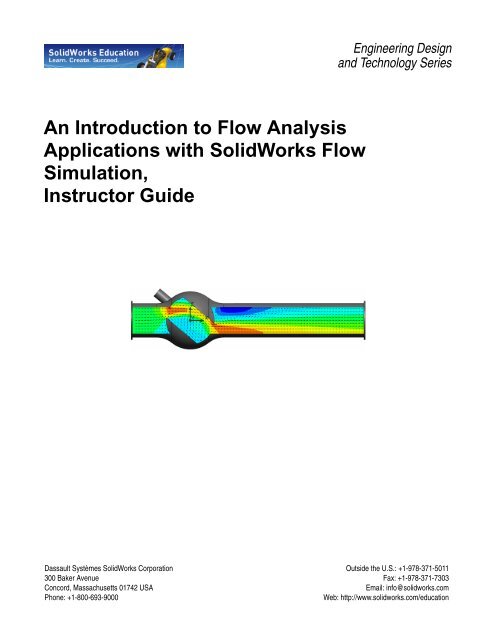
An Introduction to Flow Analysis 

Applications with SolidWorks Flow 

Simulation, 

Instructor Guide 

Dassault Systèmes SolidWorks Corporation 

300 Baker Avenue 

Concord, Massachusetts 01742 USA 

Phone: +1-800-693-9000 

Engineering Design 

and Technology Series 

Outside the U.S.: +1-978-371-5011 

Fax: +1-978-371-7303 

Email: info@solidworks.com 

Web: http://www.solidworks.com/education

© 1995-2010, Dassault Systèmes SolidWorks Corporation, a 

Dassault Systèmes S.A. company, 

300 Baker Avenue, Concord, Mass. 01742 USA. 

All Rights Reserved. 

The information and the software discussed in this document 

are subject to change without notice and are not 

commitments by Dassault Systèmes SolidWorks 

Corporation (DS SolidWorks). 

No material may be reproduced or transmitted in any form or 

by any means, electronic or mechanical, for any purpose 

without the express written permission of DS SolidWorks. 

The software discussed in this document is furnished under a 

license and may be used or copied only in accordance with 

the terms of this license. All warranties given by DS 

SolidWorks as to the software and documentation are set 

forth in the SolidWorks Corporation License and 

Subscription Service Agreement, and nothing stated in, or 

implied by, this document or its contents shall be considered 

or deemed a modification or amendment of such warranties. 

Patent Notices for SolidWorks Standard, Premium, and 

Professional Products 

U.S. Patents 5,815,154; 6,219,049; 6,219,055; 6,603,486; 

6,611,725; 6,844,877; 6,898,560; 6,906,712; 7,079,990; 

7,184,044; 7,477,262; 7,502,027; 7,558,705; 7,571,079; 

7,643,027 and foreign patents, (e.g., EP 1,116,190 and JP 

3,517,643). 

U.S. and foreign patents pending. 

Trademarks and Other Notices for All SolidWorks 

Products 

SolidWorks, 3D PartStream.NET, 3D ContentCentral, 

PDMWorks, eDrawings, and the eDrawings logo are 

registered trademarks and FeatureManager is a jointly 

owned registered trademark of DS SolidWorks. 

SolidWorks Enterprise PDM, SolidWorks Simulation, 

SolidWorks Flow Simulation, and SolidWorks 2010 are 

product names of DS SolidWorks. 

CircuitWorks, Feature Palette, FloXpress, PhotoWorks, 

TolAnalyst, and XchangeWorks are trademarks of DS 

SolidWorks. 

FeatureWorks is a registered trademark of Geometric Ltd. 

Other brand or product names are trademarks or registered 

trademarks of their respective holders. 

Document Number: PME0418-ENG 

COMMERCIAL COMPUTER 

SOFTWARE - PROPRIETARY 

U.S. Government Restricted Rights. Use, duplication, or 

disclosure by the government is subject to restrictions as set 

forth in FAR 52.227-19 (Commercial Computer Software - 

Restricted Rights), DFARS 227.7202 (Commercial 

Computer Software and Commercial Computer Software 

Documentation), and in the license agreement, as applicable. 

Contractor/Manufacturer: 

Dassault Systèmes SolidWorks Corporation, 300 Baker 

Avenue, Concord, Massachusetts 01742 USA 

Copyright Notices for SolidWorks Standard, Premium, 

and Professional Products 

Portions of this software © 1990-2010 Siemens Product 

Lifecycle Management Software III (GB) Ltd. 

Portions of this software © 1998-2010 Geometric Ltd. 

Portions of this software © 1986-2010 mental images GmbH 

& Co. KG. 

Portions of this software © 1996-2010 Microsoft 

Corporation. All rights reserved. 

Portions of this software © 2000-2010 Tech Soft 3D. 

Portions of this software © 1998-2010 3Dconnexion. 

This software is based in part on the work of the Independent 

JPEG Group. All Rights Reserved. 

Portions of this software incorporate PhysX by NVIDIA 

2006-2010. 

Portions of this software are copyrighted by and are the 

property of UGS Corp. © 2010. 

Portions of this software © 2001-2010 Luxology, Inc. All 

Rights Reserved, Patents Pending. 

Portions of this software © 2007-2010 DriveWorks Ltd 

Copyright 1984-2010 Adobe Systems Inc. and its licensors. 

All rights reserved. Protected by U.S. Patents 5,929,866; 

5,943,063; 6,289,364; 6,563,502; 6,639,593; 6,754,382; 

Patents Pending. 

Adobe, the Adobe logo, Acrobat, the Adobe PDF logo, 

Distiller and Reader are registered trademarks or trademarks 

of Adobe Systems Inc. in the U.S. and other countries. 

For more copyright information, in SolidWorks see Help > 

About SolidWorks. 

Other portions of SolidWorks 2010 are licensed from DS 

SolidWorks licensors. 

Copyright Notices for SolidWorks Simulation 

Portions of this software © 2008 Solversoft Corporation. 

PCGLSS © 1992-2007 Computational Applications and 

System Integration, Inc. All rights reserved. 

Portions of this product are distributed under license from 

DC Micro Development, Copyright © 1994-2005 DC Micro 

Development, Inc. All rights reserved.

To the Instructor 

SolidWorks Flow Simulation Instructor Guide 1 

i 

Introduction 

This document introduces SolidWorks users to the SolidWorks Flow Simulation flow and 

heat transfer analyses software package. The specific goals of this lesson are to: 

1 introduce the basic concepts of fluid flow analyses and their benefits 

2 demonstrate the ease of use and the concise process for performing these analyses 

3 introduce the basic rules for computational fluid dynamics analyses and how to obtain 

reliable and accurate results. 

This document is structured similar to lessons in the SolidWorks Instructor Guide. This 

lesson has corresponding pages in the SolidWorks Flow Simulation Student Workbook. 

Note: This lesson does not attempt to teach all capabilities of 

SolidWorks Flow Simulation. It only intends to introduce 

the basic concepts and rules of performing flow and heat 

transfer analyses and to show the ease of use and the 

concise process of doing so. 

Education Edition Curriculum and Courseware DVD 

An Education Edition Curriculum and Courseware DVD is provided with this course. 

Installing the DVD creates a folder named SolidWorks 

Curriculum_and_Courseware_2010. This folder contains directories for this 

course and several others. 

Course material for the students can also be downloaded from 

within SolidWorks. Click the SolidWorks Resources tab in the 

Task Pane and then select Student Curriculum. 

Double-click the course you would like to download. Control-select the course to 

download a ZIP file. The Lessons file contains the parts needed to complete the lessons. 

The Student Guide contains the PDF file of the course.

Introduction 

Course material for teachers can also be downloaded from the SolidWorks web site. Click 

the SolidWorks Resources tab in the Task Pane and then select Instructors Curriculum. 

This will take you to the Educator Resources page shown below. 

SolidWorks Flow Simulation Instructor Guide 2

SolidWorks Simulation Product Line 

Introduction 

While this course focuses on the introduction to flow analysis using SolidWorks Flow 

Simulation, the full product line covers a wide range of analysis areas to consider. The 

paragraphs below lists the full offering of the SolidWorks Simulation packages and 

modules. 

Static studies provide tools for the linear stress analysis of 

parts and assemblies loaded by static loads. Typical questions 

that will be answered using this study type are: 

Will my part break under normal operating loads? 

Is the model over-designed? 

Can my design be modified to increase the safety factor? 

Buckling studies analyze performance of the thin parts 

loaded in compression. Typical questions that will be answered using this study 

type are: 

Legs of my vessel are strong enough not to fail in yielding; but are they strong 

enough not to collapse due to loss of stability? 

Can my design be modified to ensure stability of the thin components in my 

assembly? 

Frequency studies offer tools for the analysis of the natural 

modes and frequencies. This is essential in the design or many 

components loaded in both static and dynamic ways. Typical 

questions that will be answered using this study type are: 

Will my part resonate under normal operating loads? 

Are the frequency characteristics of my components suitable 

for the given application? 

Can my design be modified to improve the frequency 

characteristics? 

Thermal studies offer tools for the analysis of the heat 

transfer by means of conduction, convection, and radiation. 

Typical questions that will be answered using this study type 

are: 

Will the temperatures changes effect my model? 

How does my model operate in an environment with 

temperature fluctuation? 

How long does it take for my model to cool down or overheat? 

Does temperature change cause my model to expand? 

Will the stresses caused by the temperature change cause my product failure (static 

studies, coupled with thermal studies would be used to answer this question)? 


Drop test studies are used to analyze the stress of moving 

parts or assemblies impacting an obstacle. Typical questions 

that will be answered using this study type are: 

What will happen if my product is mishandled during 

transportation or dropped? 

How does my product behave when dropped on hard wood 

floor, carpet or concrete? 

Optimization studies are applied to improve (optimize) your 

initial design based on a set of selected criteria such as maximum stress, 

weight, optimum frequency, etc. Typical questions that will be answered 

using this study type are: 

Can the shape of my model be changed while maintaining the design 

intent? 

Can my design be made lighter, smaller, cheaper without compromising 

strength of performance? 

Fatigue studies analyze the resistance of parts and assemblies 

loaded repetitively over long periods of time. Typical 

questions that will be answered using this study type are: 

Can the life span of my product be estimated accurately? 

Will modifying my current design help extend the product 

life? 

Is my model safe when exposed to fluctuating force or 

temperature loads over long periods of time? 

Will redesigning my model help minimize damage caused by fluctuating forces or 

temperature? 

Nonlinear studies provide tools for analyzing stress in parts and 

assemblies that experience severe loadings and/or large deformations. 

Typical questions that will be answered using this study type are: 

Will parts made of rubber (o-rings for example) or foam perform well 

under given load? 

Does my model experience excessive bending during normal operating 

conditions? 

Introduction 

Dynamics studies analyze objects forced by loads that vary in time. 

Typical examples could be shock loads of components mounted in 

vehicles, turbines loaded by oscillatory forces, aircraft components 

loaded in random fashion, etc. Both linear (small structural 

deformations, basic material models) and nonlinear (large structural 

deformations, severe loadings and advanced materials) are available. 

Typical questions that will be answered using this study type are: 

Are my mounts loaded by shock loading when vehicle hits a large pothole on the road 

designed safely? How much does it deform under such circumstances? 


Motion Simulation enables user to analyze the kinematic and dynamic 

behavior of the mechanisns. Joint and inertial forces can subsequently be 

transferred into SolidWorks Simulation studies to continue with the 

stress analysis. Typical questions that will be answered using this 

modulus are: 

What is the correct size of motor or actuator for my design? 

Is the design of the linkages, gears or latch mechanisms optimal? 

What are the displacemements, velocities and accelerations of the mechanism 

components? 

Is the mechanism efficient? Can it be improved? 

Composites modulus allows users to simulate structures 

manufactured from laminated composite materials. 

Typical questions that will be answered using this modulus are: 

Is the composite model failing under the given loading? 

Can the structure be made lighter using composite materials 

while not compromising with the strength and safety? 

Will my layered composite delaminate? 

Introduction 


Goals of This Lesson 

Basic Functionality of SolidWorks Flow Simulation 

Introduce flow analysis as a tool predicting characteristics of various flows over and 

inside 3D objects modeled by SolidWorks and thereby solving various hydraulic and 

gas dynamic engineering problems. Upon successful completion of this lesson, the 

students should understand basic approaches to solving hydraulic and gas dynamic 

engineering problems. The students should see that the analysis of the flow over 

complex objects can influence the objects' design and performance, significantly save 

time and money by performing a properly stated comprehensive CFD analysis with 

SolidWorks Flow Simulation instead of conducting extremely time-consuming and 

expensive experimental works. 

Associate SolidWorks Flow Simulation flow analysis as "a chess game", in which it is 

very easy "to arrange the figures over the board before the game", some effort is 

required "to obey the game rules", and it will be necessary to apply some strategy "to 

win the game", i.e. to obtain correct and accurate results. The students should see that, 

due to SolidWorks Flow Simulation's clear and well-structured interface, it is relatively 

easy "to arrange the figures over the board before the game", therefore the user will 

have more time to develop a strategy of solving the engineering problem, specify the 

boundary conditions properly, and study the obtained results for a possible change in 

strategy. So, this step shows how "to arrange the figures over the board before the 

game" in SolidWorks Flow Simulation. 

Show the students the proper ways of correctly simulating real objects and flow 

phenomena with SolidWorks Flow Simulation. 

The results of analysis may vary slightly depending on versions/builds of SolidWorks 

and SolidWorks Flow Simulation. 


2

Outline 

In Class Discussion 

Active Learning Exercise — Determination of Hydraulic Loss 

• Opening the Valve.SLDPRT Document 

• Checking the SolidWorks Flow Simulation menu 

• Model Description 

• Creating Lids Manually 

• Creating Lids Automatically 

• Creating a Project 

• SolidWorks Flow Simulation Design Tree 

• Specifying Boundary Conditions 

• Specifying Surface Goals 

• Specifying the Equation Goal 

• Running the Calculation 

• Monitoring the Solver 

• Accessing the Results 

• Creating a Cut Plot 

• Displaying Flow Trajectories 

• Creating a Goal Plot 

• Cloning Project 

• Changing the Valve Angle 

• Changing the Geometry Resolution 

• Changing the Computational Domain 

• Getting the Valve’s Hydraulic Loss 

5 Minute Assessment – Answer Key 

In Class Discussion — Changing the Inlet Boundary Condition 

More to Explore — Modifying the Geometry 


Exercises and Projects — Hydraulic Loss Due to Sudden Expansion 

Lesson Summary 


In Class Discussion 


Ask students where a fluid flow and heat transfer analysis software can be beneficial for a 

design engineer? 

Answer 

Machinery: Hydraulic/pneumatic systems manufacturers can improve their designs regarding 

flow distribution and pressure drop. Oil industry can better understand flow through valves or 

mixing vessels, etc. Particle tracking can be used to understand how safe equipment is against 

erosion. 

Electrical and Electronics: Designers of electronic devices (computers, audio/video, etc.) can 

check for efficient cooling by simulating convection and conduction within their designs. 

Aerospace and Automotive: Land-, air- and marine-vehicle designers can achieve maximum 

performance, at least cost: Manifolds, brake systems, engine cooling jacket, flow around a wing 

or through a rocket nozzle, flow around an immersed body etc. 

HVAC & Building: HVAC equipment manufactures can optimize product performance: flow 

through ducts, heat exchangers, flow and temperature distributors in rooms to determine duct 

locations, etc. 

Consumer Products: Consumer products designers can improve the uniform distribution in an 

oven or correct the flow distribution in a dishwasher etc. 

Design engineers, analysts, and other professionals can recognize forces and torques and other 

loads acting on objects due to the fluid flow and use this knowledge in further structural analysis 

for achieving the better designs. 

More to explore 

Regarding structural analysis, ask the students how the forces acting on a particular object 

(whose stress is analyzed within SolidWorks Simulation) was determined. Are these 

forces always known or estimated from known formulas? 

Answer 

In some problems, even involving fluids, these forces are either well known or can be neglected. 

For example, a force acting on the chair's legs is determined as the weight of the student sitting 

on it in a room plus the chair's weight, or a force and moment acting on a manually operated 

small valve can be neglected. But determining the forces on many problems in industry are just 

too complicated and computer computations will be required to determine the needed forces. For 

example, if the valve is large, e.g. as used for hydroelectric power stations, both the force and the 

moment acting on the valve from the fluid must be certainly taken into account, otherwise the 

valve's parts (e.g. bearings) and devices (e.g. actuators turning the valve) can fail, so the valve 

becomes inoperative. 


Active Learning Exercise — Determination of Hydraulic Loss 

Use SolidWorks Flow Simulation to perform 

fluid internal analysis on the Valve.SLDPRT 

part shown to the right. 

The step-by-step instructions are given below. 


Opening the Valve.SLDPRT Document 

1 Click File, Open. In the Open dialog box, browse to the Valve.SLDPRT part located 

in the corresponding subfolder of the SolidWorks 

Curriculum_and_Courseware_2010 folder and click Open (or double-click 

the part). 

Checking the SolidWorks Flow Simulation Menu 

If SolidWorks Flow Simulation is properly 

installed, the Flow Simulation menu 

appears on the SolidWorks menu bar. If 

not: 

1 Click Tools, Add-Ins. 

The Add-Ins dialog box appears. 

2 Check the checkboxes next to SolidWorks Flow Simulation. 

If SolidWorks Flow Simulation is not in the list, you need to install SolidWorks Flow 

Simulation first. 

3 Click OK. The Flow Simulation menu appears on the SolidWorks menu bar. 

Model Description 

This is a ball valve. Turning the handle closes or 

opens the valve. 

The local hydraulic loss (or resistance) produced by a 

ball valve installed in a piping system depends on the 

valve design dimensions and on the handle turning 

angle. The ball-to-pipe diameter ratio governs the 

handle turning angle at which the valve becomes 

closed. 

handle 

SolidWorks Flow Simulation 


Inlet 

Outlet


The standard engineering definition of a hydraulic resistance of an obstacle in a pipe is the 

difference between the total pressures (i.e. where a stream is not disturbed by the obstacle) 

upstream and downstream of the obstacle (the valve in our case) divided by the incoming 

dynamic head, from which the hydraulic resistance due to the friction over the pipe section 

is subtracted. 

In this example we will obtain the local hydraulic resistance of the ball valve whose 

handle is turned by an angle of 40 o . The Valve analysis represents a typical SolidWorks 

Flow Simulation internal analysis. 

Note: Internal flow analyses are analyses where fluid enters a model at the inlets 

and exits the model through the outlets. The exception are some natural 

convection problems that may not have openings. 

To perform an internal analysis all the model openings must be closed with lids, which are 

needed to specify inlet and outlet flow boundary conditions on them. In any case, the 

internal model space filled with a fluid must be fully closed. The lids are simply additional 

extrusions covering the openings. They can be created both manually and automacially; 

both of the procedures are shown below. 

Creating Lids Manually 

Creating Inlet Lid 

1 Select the face shown in the picture. 

2 Click Sketch on the Sketch toolbar. 

3 Select the tube’s inner edge. 

4 Click Convert Entities on the Sketch toolbar. 

5 Complete the sketch by clicking OK button in the confirmation 

corner of the graphics area. 

6 Click Extruded Boss/Base on the Features toolbar. 

7 In the Extrude Feature PropertyManager change the settings as 

shown. 

• End Condition = Mid Plane 

• Depth = 0.005m 

8 Click to create the inlet lid. 

Next, in the same manner we will create the outlet lid. 


Creating Outlet Lid 

9 Select the face shown in the picture. 

10 Click Sketch on the Sketch toolbar. 

11 Select the tube’s inner edge. 

12 Repeat the steps 3 to 8 to create the lid at outlet. 

13 Rename the new extrusions Extrude1 and Extrude2 to 

Inlet Lid and Outlet Lid, correspondingly. 


Not sure you have created the lids properly? SolidWorks Flow Simulation can easily 

check your model for possible geometry problems. 

Checking the Geometry 

1 To ensure the model is fully closed, click Flow Simulation, 

Tools, Check Geometry. 

2 Click Check to calculate the fluid volume of the model. If the 

fluid volume is equal to zero, the model is not closed properly. 

Note: This Check Geometry tool allows you to 

calculate the total fluid and solid volumes, 

check bodies for possible geometry 

problems (i.e. tangent contact) and 

visualize the fluid area and solid body as 

separate models. 

Creating Lids Automatically 

The previous step showed the manual lid creation. In the next step you will practice the 

SolidWorks Flow Simulation automatic lid creation tool. This tool can save considerable 

amount of time if multiple lids are needed to close the internal volume. 

Deleting manually created lids 

Delete Inlet Lid and Outlet Lid features. 

Creating Inlet and Outlet Lids 

1 Click Flow Simulation, Tools, Create Lids. 

The Create Lids dialog box appears. 


2 Select the two inlet 

and outlet faces 

shown in the figure. 

3 Click to 

complete the lid 

definitions. 

4 Rename the newly 

created features 

LID1 and LID2 to 

Inlet Lid and Outlet Lid, respectively. 


The first step in performing flow analysis is to create a SolidWorks Flow Simulation 

project. 

Creating a Project 

Note: In the assembly mode, each newly created lid forms a new part saved in 

the assembly folder. 

1 Click Flow Simulation, Project, Wizard. The project wizard guides you through the 

definition of a new SolidWorks Flow Simulation project. 

2 In the Project Configuration dialog box, 

click Use current (40 degrees). 

Each SolidWorks Flow Simulation project 

is associated with a SolidWorks 

configuration. You can attach the project 

either to the current SolidWorks 

configuration or create a new SolidWorks 

configuration based on the current one. 

Click Next. 

3 In the Unit System dialog box you can 

select the desired system of units for both 

input and output (results). 

For this project we accept the default 

selection of SI (International System). 

Click Next. 


4 In the Analysis Type dialog box you can 

select either Internal or External type of 

the flow analysis. This dialog also allows 

you to specify advanced physical features 

you want to take into account: heat transfer 

in solids, surface-to-surface radiation, 

time-dependent effects, gravity and 

rotation. 

Specify Internal type and accept the 

default values for the other settings. Click 

Next. 

5 In the Default Fluid dialog box you can 

select the fluid type. The selected fluid 

type is assigned by default for all fluids in 

the analysis. 

Click Liquids and then double-click the 

Water item in the Liquids list. 

Leave defaults under Flow 

Characteristics and click Next. 

6 In the Wall Conditions dialog box you 

can specify the wall roughness value and 

the wall thermal condition. 

In this project we will not deal with the 

rough walls and heat conduction through 

the walls, so leave the default settings and 

click Next. 


Note: The SolidWorks Flow Simulation Engineering Database contains 

physical properties of predefined and user-defined gases, real gases, 

incompressible liquids, non-Newtonian liquids, compressible liquids, 

solid substances and porous materials. It includes both constant values 

and tabular dependencies of various physical parameters on temperature 

and pressure. 

The Engineering Database also contains unit systems, values of thermal 

contact resistance for various solid materials, properties of radiative 

surfaces and integral physical characteristics of some technical devices, 

namely, fans, heat sinks, and thermoelectric coolers. You can easily 

create your own substances, units, fan curves or specify a custom 

parameter you want to visualize. 


7 In the Initial Conditions dialog box 

specify initial values of the flow 

parameters. For steady internal problems, 

the values specified closer to the expected 

flow field will reduce the analysis time. 

For this project use the default values. 

Click Next. 


Note: For steady flow problems SolidWorks Flow Simulation iterates until the 

solution converges. For unsteady (transient, or time-dependent) problems 

SolidWorks Flow Simulation marches in time for a period you specify. 

8 In the Results and Geometry Resolution 

dialog box you can control the analysis 

accuracy as well as the mesh settings and, 

by this, the required computer resources 

(CPU time and memory). 

For this project accept the default Result 

resolution level 3. 

Result resolution governs the solution 

accuracy that can be interpreted as 

resolution of calculation results. You 

specify result resolution in accordance with 

the desired solution accuracy, available CPU time and computer memory. Because this 

setting has an influence on the number of generated mesh cells, a more accurate 

solution requires longer CPU time and more computer memory. 

Geometry Resolution (specified through the Minimum gap size and the Minimum 

wall thickness) governs proper resolution of geometrical model features by the 

computational mesh. Naturally, finer geometry resolution requires more computer 

resources. 



Select the Manual specification of the minimum gap size check box and enter 

0.04 m for the minimum flow passage. 

Click Finish. 

SolidWorks Flow Simulation Design Tree 

After the basic part of the project has been created, a new SolidWorks Flow Simulation 

design tree tab appears on the right side of the Configuration Manager tab. 

At the same time, in the SolidWorks graphics area a 

computational domain wireframe box appears. The flow 

and heat transfer calculations are performed inside the 

computational domain. The computational domain is a 

rectangular prism for both the 3D and 2D analyses. The 

computational domain boundaries are parallel to the 

global coordinate system planes. 

Now let us specify the other parts of the project. 

0.04 m 

Note: SolidWorks Flow Simulation calculates the default minimum gap size 

and minimum wall thickness using information about the overall model 

dimensions, the computational domain, and faces on which you specify 

conditions and goals. However, this information may be insufficient to 

recognize relatively small gaps and thin model walls. This may cause 

inaccurate results. In these cases, the Minimum gap size and Minimum 

wall thickness must be specified manually. 

Note: The SolidWorks Flow Simulation Design Tree provides a convenient 

specification of project data and view of results. You also can use the 

SolidWorks Flow Simulation design tree to modify or delete the various 

SolidWorks Flow Simulation features. 

computational domain 

The next step is the specifycation of the boundary conditions. Boundary conditions are 

used to specify the fluid characteristics at the model inlets and outlets in an internal flow 

analysis or on model surfaces in an external flow analysis. 


Specifying Boundary Conditions 

1 Click Flow Simulation, Insert, Boundary Condition. 

2 Select the Inlet Lid inner face (in contact with the fluid). 

To access the inner face, right-click the lid’s outer face and 

choose Select Other. Right-click the mouse to cycle through 

the faces under the cursor until the inner face is highlighted, 

then click the left mouse button. 

The selected face appears in the Faces to Apply the 

Boundary Condition list. 

3 In the Type group box, click Flow Openings and select the 

Inlet Velocity item. 

4 In the Flow Parameters group box, click Normal to Face item 

and set the Velocity Normal to Face to 1 m/s (just type the 

value, the units will appear automatically). 

Accept all other parameters and click . 

By specifying this condition we define that the water enters the valve 

at the ball valve pipe inlet with the velocity of 1.0 m/s. 

5 Select the Outlet Lid inner face. 

In the graphics area, right-click outside the model and 

select Insert Boundary Condition. The Boundary 

Condition PropertyManager appears with the selected 

face in the Faces to Apply the Boundary Condition 

list. 


Let us specify pressure on this boundary, otherwise the problem specification is deficient. 

Before the calculation starts, SolidWorks Flow Simulation checks the specified boundary 

conditions for mass flow rate balance. The specification of boundary conditions is 

incorrect if the total mass flow rate on the inlets is not equal to the total mass flow rate on 

the outlets. In such case the calculation will not start. Also, note that the mass flow rate 

value is recalculated from the velocity or volume flow rate value specified on an opening. 

Specifying at least one Pressure opening condition allow us to avoid problems with mass 

flow rate balance, since the mass flow rate on a Pressure opening is not specified but 

calculated during the problem solution. 


6 Click Pressure Openings and in the Type of Boundary 

Condition list select the Static Pressure item. 

7 Accept the default values for all of the other parameters (101325 

Pa for Static Pressure, 293.2 K for the Temperature, for 

example). 

8 Click . 


By specifying this condition we define that the water has a static pressure of 1 atm at the 

ball valve pipe exit. 

The model’s hydraulic loss ξ is calculated as the difference between the model’s inlet total 

pressure and the outlet total pressure, ΔP, divided by the dynamic pressure (dynamic head) 

determined at the model inlet: 

where ρ is water density, V is water inlet velocity, Pdyn is the dynamic pressure at inlet. 

Since we already know the specified water velocity (1 --- ) and the water density (998.1934 

kg 

m 3 

------ 

for the specified temperature of 293.2 K), our goal is to determine the total pressure 

value at the valve’s inlet and outlet. 

ξ ( dP) 

ρV2 

= ⁄ --------- = ( dP) 

⁄ P 

2 

dyn 

The easiest and fastest way to find the parameter of interest is to specify the corresponding 

engineering goal. 

Engineering goals are the parameters which the user is interested in. Setting goals is 

essentially a way of conveying to SolidWorks Flow Simulation what you are trying to get 

out of the analysis, as well as means of reducing the time SolidWorks Flow Simulation 

takes to reach a solution. By only selecting the variable which the user desires accurate 

values for, SolidWorks Flow Simulation knows which variables are important to converge 

upon (the variables selected as goals) and which can be less accurate (the variables not 

selected as goals) in the interest of time. Goals can be defined over the entire domain 

(Global Goals), within a selected volume (Volume Goal), on a selected area (Surface 

Goal) or at a specific point of the model (Point Goal). Furthermore, SolidWorks Flow 

Simulation can consider either average, minimum or maximum parameter value to define 

the goal. You can also define an Equation Goal that is a goal defined by an equation 

(involving basic mathematical functions) with the existing goals as variables. The 

equation goal allows you to calculate the parameter of interest (i.e., pressure drop) and 

keeps this information in the project for later reference. 


m 

s

Specifying Surface Goals 

1 In the SolidWorks Flow Simulation design tree, rightclick 

the Goals icon and select Insert Surface Goal. 

2 Select the inner face of the Inlet Lid. 

To easily select a face, simply click the 

Inlet Velocity 1 item in the SolidWorks Flow 

Simulation design tree. The face related to the specified 

boundary condition is automatically selected and appears 

in the Faces to Apply the Surface Goal list. 

3 In the Parameter list, find Total Pressure. Click in the 

Av column to use the average value and keep selected 

Use for conv. to use this goal for the convergence 

control. 


Note: To see the parameter names more clearly, you will probably find useful 

to enlarge the PropertyManager area by dragging the vertical bar to the 

right. 

4 Click . 

5 In the SolidWorks Flow Simulation design tree click-pause-click the new 

SG Av Total Pressure 1 item and rename it to SG Average Total 

Pressure Inlet. 

Note: Another way to rename an item is to right-click the item and select 

Properties. 

6 Right-click the Goals icon again and select Insert Surface Goal. 

7 Click the Static Pressure 1 item in the SolidWorks Flow Simulation design tree 

to select the inner face of the Outlet Lid. 

8 In the Parameter list, find Total Pressure. 

9 Click in the Av column and then click . 

10 Click-pause-click the new SG Av Total Pressure 1 item and rename it to SG 

Average Total Pressure Outlet. 

11 Right-click the Goals icon again and select Insert Surface Goal. 

12 Click the Inlet Velocity 1 item to select the inner face of the Inlet Lid. 

13 In the Parameter list, find Dynamic Pressure. 

14 Click in the Av column and then click . 

15 Click-pause-click the new SG Average Dynamic 

Pressure1 item and rename it to SG Average 

Dynamic Pressure Inlet. 



The value of the dynamic pressure at the inlet can be calculated manually. We have 

specified the dynamic pressure goal just for the convenience of the further calculation of 

hydraulic losses. 

After finishing the calculation you will need to manually calculate the hydraulic loss ξ 

from the obtained total pressures values. Instead, let SolidWorks Flow Simulation make 

all the necessary calculations for you by specifying an Equation Goal. 

Specifying the Equation Goal 

Equation Goal is a goal defined by an analytical function of the existing goals. This goal 

can be monitored during the calculation and while displaying results in the same way as 

the other goals. Any of the existing goals can be used as variables, including other 

equation goals, except those that are dependent on other equation goals. You can also use 

constants in the definition of the equation goal. 

1 Right-click the Goals icon and select Insert 

Equation Goal. The Equation Goal dialog box 

appears. 

2 Click the left bracket button or type “(“. 

3 In the Goals list select the SG Average 

Total Pressure Inlet goal. The goal is 

then automatically added in the Expression 

field. 

4 Click the minus button or type "-". 

5 In the Goals list select the SG Average 

Total Pressure Outlet goal. 

6 Click the right bracket and the forward slash buttons, or type ")/". 

7 In the Goals list select the SG Average Dynamic Pressure Inlet goal 

name. 

8 In the Dimensionality list select No units. 

Note: To set an Equation Goal you can use only existing goals (including 

previously specified Equation Goals) and constants. If constants signify 

some physical parameters (i.e. length, area etc.) make sure of using the 

project’s system of units. SolidWorks Flow Simulation has no 

information about the physical meaning of the specified constants so you 

need to specify the displayed dimensionality manually. 

9 Click OK. The Equation Goal 1 item appears in the tree. 

10 Rename it to Hydraulic Loss. 



Now the SolidWorks Flow Simulation project is ready for the calculation. SolidWorks 

Flow Simulation will finish the calculation when the steady-state average value of total 

pressure calculated at the valve inlet and outlet are reached. 

Running the Calculation 

1 Click Flow Simulation, Solve, Run. The Run dialog 

box appears. 

2 Click Run to start the calculation. 

The calculation should take about 2 minutes to run on a 

2.26 GHz Pentium M computer. 

SolidWorks Flow Simulation 

automatically generates a computational 

mesh in accordance with your settings 

of Result resolution and Geometry 

resolution. The mesh is created by 

dividing the computational domain into 

cells, i.e. elementary rectangular 

volumes. The cells are further 

subdivided as necessary to resolve 

properly the model geometry and flow 

features. This process is called mesh 

refinement. During the mesh generation 

procedure, you can see the current step 

and the mesh information in the Mesh Generation dialog box. 

Monitoring the Solver 

This is the solution monitor dialog box. 

To the left you may see the stepwise log 

of the solution process. The information 

dialog box arranged to the right contains 

summary information on the mesh and 

any warnings on different issues that 

may arise during the analysis. 

During the calculation you can monitor 

the convergence behavior of your goals 

(Goal Plot), view the current results in 

the specified plane (Preview) and 

display the minimum and maximum 

parameter values at the current iteration 

(Min/Max table). 


Creating Goal Plot 


1 Click Insert Goal Plot 

box appears. 

on the Solver toolbar. The Add/Remove Goals dialog 

2 Click Add All to check all goals and click OK. 

This is the Goal Plot dialog box. All added goals 

together with their current values are listed at the 

top part of the window, as well as the current 

progress towards completion given as a 

percentage. The progress value is only an 

estimate and generally (but not necessarily) 

increases with time. Below you can see the graph 

of all goals. 

Convergence is an iterative process. The 

discretization of the flow field imposes conditions 

on each parameter and each parameter cannot reach an absolutely stable value but will 

oscillate near this value from iteration to iteration. When SolidWorks Flow Simulation 

analyzes the goal's convergence, it calculates the goal's dispersion defined as the 

difference between the goal's maximum and minimum values over the analysis interval 

reckoned from the last iteration and compares this dispersion with the goal's convergence 

criterion dispersion, either specified by you or automatically determined by SolidWorks 

Flow Simulation. Once the oscillations are less than the convergence criterion the goal 

becomes converged. 

Preview Results 

1 While the calculation is still running, click Insert 

Preview on the Solver toolbar. The 

Preview Settings dialog box appears. 

2 Click the FeatureManager tab . 

3 Select Plane 2. 

For this model Plane 2 is a good choice to use as the preview 

plane. The preview plane can be chosen anytime from the Feature 

Manager. 



4 Click OK to display the preview plot of the static pressure distribution. 

Note: You can specify a parameter you want to display in the preview plane, 

the parameter range and display options for velocity vectors at the 

Setting tab of the Preview Settings dialog box. 

The preview allows one to look at the results 

while the calculation is still running. This 

helps to determine if all the boundary 

conditions are correctly defined and gives the 

user idea of how the solution will look even 

at this early stage. 

At the start of the run the results might look odd or change abruptly. However, as the 

run progresses these changes will lessen and the results will settle in on a converged 

solution. The result can be displayed either in contours, isolines or vector 

representation. 

Note: Why does the static pressure increase at the local region inside the valve? 

This is due to a deceleration (up to stagnation within a small region) of 

the stream impacting the valve’s wall in this region, so the stream’s 

dynamic pressure is partly transformed into the static pressure while the 

stream’s total pressure is nearly constant in this region, so the static 

pressure rises. 

5 When the solver is finished, close the monitor by clicking File, Close. 

Accessing the Results 

Expand the Results folder in the project tree by clicking the corresponding (+) sign. 

Note: When the solver is finished, the results are loaded automatically (unless 

the Load results check box in the Run window has been unchecked). 

However, when working with a previously calculated project, you need 

to load the results manually by clicking Flow Simulation, Results, 

Load/Unload Results. 

Once the calculation finishes, you can view the saved calculation results in numerous 

ways and in a customized manner directly within the graphics area. The Result folder 

features functions that may be used to view your results: Cut Plots (section views of 

parameter distribution), 3D-Profile Plots (section views in relief representation), 

Surface Plots (distribution of a parameter on a selected surface), Isosurfaces, 

Flow Trajectories, Particle Studies (particle trajectories), XY Plots 

(diagrams of parameter behavior along a curve or sketch), Point Parameters 

(getting parameters at specified points), Surface Parameters (getting parameters at 

specified surfaces), Volume Parameters (getting parameters within specified 

volumes), Goals (behavior of the specified goals during the calculation), Reports 

(export of project report output into MS Word) and Animation of results. 


Creating a Cut Plot 


1 Right-click the Cut Plots icon and select Insert. The Cut Plot dialog box appears. 

The Cut Plot displays results of a selected parameter in a selected 

view section. To define the view section, you can use SolidWorks 

planes or model planar faces (with the additional shift if 

necessary). The parameter values can be represented as a contour 

plot, isolines, vectors, or in a combination (e.g. contours with 

overlaid vectors). 

2 Click the SolidWorks FeatureManager and select Plane2. Its 

name appears in the Section Plane or Planar Face list on the 

Selection tab. 

3 In the Cut Plot PropertyManager window, in addition to 

displaying Contours , click Vectors . 

4 In the Vectors group box, using the slider set the Vector Spacing 

to approximately 0.012 m. 

5 Click View Settings in order to specify the parameter which will 

be shown in the contour plot. 

Note: The settings made in the View Settings dialog box refer to all cut plots, 

surface plots, isosurfaces and flow trajectories specific features. These 

settings are only applied for the active pane of the SolidWorks graphics 

area. For example, the contours in all cut and surface plots will show the 

same physical parameter selected in the View Settings dialog box. So, in 

the View Settings dialog box for each of the displaying options 

(contours, isolines, vectors, flow trajectories, isosurfaces) you specify 

the displayed physical parameter and the settings required for displaying 

it through this option. The contour settings can also be applied to 

isolines, vectors, flow trajectories and isosurfaces. 

6 On the Contours tab, in the Parameter box 

select X-Component of Velocity. 

7 Click OK to save changes and close the View 

Settings dialog box. 

8 Click to create the cut plot. The new 

Cut Plot 1 item appears in the SolidWorks 

Flow Simulation design tree. 

However, the cut plot is not seen through the model. In order to see the plot, you can hide 

the model by clicking Flow Simulation, Results, Display, Geometry (alternatively, you 

can use the standard SolidWorks Section View option) or change the model transparency 

(as is done in the next step below). 


9 Click the Flow Simulation, Results, Display, Geometry 

to show the model. Click Flow Simulation, Results, 

Display, Transparency and drag the slider to set the value 

of approximately 0.85. 

Click . 

10 In the SolidWorks Flow Simulation design tree, right-click 

the Computational Domain icon and select Hide. 

Now you can see a contour plot of the velocity and the velocity 

vectors projected on the plot. 

For better visualization of the vortex you can scale small vectors: 

11 In the SolidWorks Flow Simulation design tree, rightclick 

the Results icon and select View Settings. 

12 In the View Settings dialog, click the Vectors 

tab and type 0.02 m in the Arrow size box. 

13 Change the Min value to 2 m/s. 

By specifying the custom Min we change the 

vector length so the vectors whose velocity is 

less than the specified Min value will have the 

same length as the vectors whose velocity is 

equal to the Min. This allows us to visualize 

the low velocity area in more details. 




14 Click OK to save the changes and exit the View Settings dialog box. Immediately the 

cut plot is updated. 

Displaying Flow Trajectories 

With the use of Flow trajectories you can show the flow streamlines. Flow streamlines 

provide a very clear and comprehensible representation of the flow peculiarities. You can 

also see how parameters change along each trajectory by exporting data into Excel. 

Additionally, you can save trajectories as SolidWorks reference curves. 

Right-click the Cut Plot 1 icon and select Hide. 

1 Right-click the Flow Trajectories icon and select Insert. The Flow Trajectories 

dialog box appears. 

2 In the SolidWorks Flow Simulation Design Tree, click the 

Static Pressure 1 item to select the inner face of the Outlet 

Lid. Trajectories launched from the outlet opening will better 

visualize the vortex occurring downstream the valve’s obstacle. 

3 Set the Number of trajectories to 50. 

4 Click the Constraints tab and decrease the Maximum length of 

trajectories to 2 m. 

5 Click OK to display trajectories. 

6 

Some may prefer to display the flow trajectories with the help of a section plot. Use 

Plane2 to define a section plot to show the flow trajectories. 



Rotate the model to examine the 3D structure of the vortices in more detail. 

Creating a Goal Plot 

The Goal Plot allows you to study the goal changes in the course of the calculation. 

SolidWorks Flow Simulation uses Microsoft Excel to display the goal plot data. Each goal 

plot is displayed in a separate sheet. The converged values of all project goals are 

displayed in the Summary sheet of an automatically created Excel workbook. 

1 In the SolidWorks Flow Simulation design tree, under Results, 

right-click the Goals icon and select Insert. The Goals dialog box 

appears. 

2 Click Add All. 

3 Click OK. The goals1 Excel workbook is 

created. 

This workbook displays how the goal values had 

changed during the calculation. You can take the 

total pressure value presented in the Summary 

sheet. 

Cloning Project 

The current calculation yields the total hydraulic resistance ξ including both valve's 

hydraulic resistance ξν (due to the obstacle) and the tubes' hydraulic resistance due to 

friction ξ f : ξ = ξν + ξ f . To obtain the valve’s resistance, it is necessary to subtract from the 

obtained data the total pressure loss due to friction in a straight pipe of the same length and 

diameter. To do that, we will perform the same calculations in the ball valve model whose 

handle is turned by an angle of 0 o . 



You can create a new SolidWorks Flow Simulation project in three ways: 

• The Project Wizard is the most straightforward way of creating a SolidWorks Flow 

Simulation project. It guides you step-by-step through the analysis set-up process. 

• To analyze different flow or model variations, the most efficient method is to clone 

(copy) your current project. The new project will have all the settings of the cloned 

project, optionally including the results settings. 

• You can create a SolidWorks Flow Simulation project by using a Template, either a 

default template or custom template created from a previous SolidWorks Flow 

Simulation project. Template contains only general project settings (the settings you 

specify in the Wizard and General Settings only) and does not contain the other project 

features like boundary conditions, goals, etc. 

The easiest way to create a new SolidWorks configuration for 0 o angle and specify the 

same condition as the 40 o angle project is to clone the existing 40 project. 

1 Click Flow Simulation, Project, Clone Project. 

2 Click Create New. 

3 In the Configuration name box, type 00 degrees. 

4 Click OK. 

Now the new SolidWorks Flow SimulationSolidWorks Flow 

Simulation project is attached to the new 00 degrees configuration and has inherited 

all the settings from the 40 degrees project. All our input data are copied, so we do not 

need to redefine them. All changes will only be applied to this new configuration, not 

affecting the old project and its results. 

Changing the Valve Angle 

1 In the SolidWorks 

FeatureManager, right-click 

the Angle Definition 

feature and select Edit 

Feature. 

2 In the At angle box, type 

90. 

3 Click OK . 

After clicking OK, two warning messages appear asking you to rebuild the 

computational mesh and to reset the computational domain. 


4 Answer Yes to the both messages. 

Changing the Geometry Resolution 


Since at the zero angle the ball valve becomes a simple straight pipe, there is no need to set 

the Minimum gap size value smaller than the default gap size which, in our case, is 

automatically set equal to the pipe’s diameter (the automatic minimum gap size depends 

on the characteristic size of the faces on which the boundary conditions are set). Note that 

using a smaller gap size will result in a finer mesh which, in turn, will require more 

CPU time and memory. To solve your task in the most effective way you should choose 

the optimal settings for the task. 

1 Click Flow Simulation, Initial Mesh. 

2 Clear the Manual specification of the 

minimum gap size check box. 

3 Click OK. 

Changing the Computational Domain 

You can take advantage of the symmetry 

of the straight pipe to reduce the CPU time and 

memory requirements for the computation. Since the 

flow is symmetric at two directions (Y and Z), it is 

possible to “cut” the model in one fourth and use a 

symmetry boundary condition on the planes of 

symmetry. This procedure is not required but is 

recommended for efficient analyses. 

Symmetry 

Note: The symmetric conditions can be applied only if you are sure that the 

flow is symmetric. Note that sometimes symmetry of both the model and 

the incoming flow does not guarantee symmetry in other flow regions, 

e.g. a von Karman vortex street behind a cylinder. In our case, the flow in 

the straight pipe is symmetric so we can reduce the computational 

domain. 

1 In the SolidWorks Flow Simulation design tree right-click the Computational 

Domain icon and select Edit Definition. The Computational Domain dialog box 

appears. 

In the Computational Domain dialog box you can perform the following: 

• Resize the Computational Domain. 

• Apply the Symmetry boundary condition. The flow symmetry planes can be utilized 

as computational domain boundaries with specified Symmetry conditions on them. 



In this case, the computational domain boundaries must coincide with the flow 

symmetry planes. 

• Specify a 2D plane flow. If you are fully confident that the flow is a 2D plane flow, 

you can redefine the computational domain from the default 3D analysis to a 2D 

plane flow analysis that results in decreases in memory and CPU time requirements. 

To activate a 2D planar analysis, select 2D plane flow on the Boundary Condition 

tab. 

2 In the Y min box type 0. 

3 In the Z min box type 0. 

4 Click the Boundary Condition tab. 

5 In the At Y min and At Z min lists select Symmetry. 

6 Click OK. 

7 Click Flow Simulation, Solve, Run. Then click 

Run to start the calculation. 

Getting the Valve’s Hydraulic Loss 

After the calculation is finished, close the monitor dialog box and create the goal plot with 

the newly obtained results. 

Now you can calculate the valve’s hydraulic loss in the ball valve whose handle is turned 

by 40 o . To determine the parameter's steady-state value more accurately, it would be more 

accurate to use the values averaged over the analysis interval, which are shown in the 

Averaged Value column. 

Total hydraulic losses (40 deg) Friction losses (0 deg) Valve’s loss 

Save Your Work and Exit SolidWorks 

20.6 0.20 20.4 

1 Click on the Standard toolbar or click File, Save. 

2 Click File, Exit on the Main menu. 


5 Minute Assessment – Answer Key 

1 What is SolidWorks Flow Simulation? 


Answer: SolidWorks Flow Simulation is a fluid flow and heat transfer analysis product 

fully integrated within SolidWorks. 

2 How do you start a SolidWorks Flow Simulation session? 

Answer: On the Windows task bar, click Start, Programs, SolidWorks, SolidWorks 

Application. The SolidWorks application starts. 

3 What is a fluid flow analysis? 

Answer: Fluid flow analysis is a process to simulate how the fluid influences the design 

and performance of your device or to simulate how a device affects the fluid flow 

parameters. 

4 Why analysis is important? 

Answer: Analyses enables you to understand and improve your design saving your time 

and money by reducing traditional design cycle. 

5 What kind of analyses is typical for SolidWorks Flow Simulation internal flow 

analyses? 

Answer: Typical internal analyses are those when the fluid enters a model at the model 

inlets and exits the model through outlets. 

6 What is the specific requirement of SolidWorks Flow Simulation internal analyses? 

Answer: SolidWorks Flow Simulation internal analyses require that the models be fully 

closed. 

7 How can you ensure the model is closed? 

Answer: You can calculate the model’s internal volume by using the Check Geometry 

tool. If the volume is zero, your model is not closed. 

8 Why is it necessary to add lids to the ball valve model openings? 

Answer: Lids make the model closed for an internal analysis. You will need to apply 

inlet and outlet boundary conditions on the lids. 

9 What is the first step to start a SolidWorks Flow Simulation analysis? 

Answer: The first step to start a SolidWorks Flow Simulation analysis is to create a 

SolidWorks Flow Simulation project. 

10 In what ways can a SolidWorks Flow Simulation project be created? 

SolidWorks Flow Simulation project can be created in one of the three ways: 

• use the Project Wizard. 

• use the template. 

• clone an existing project. 

11 How do you specify a fluid for a project? 

Answer: To specify a fluid for a project, select the fluid from a list of fluids in the 

SolidWorks Flow Simulation Engineering Database from the Wizard (or General 

Settings) dialog box. 

12 How does a user define a fluid entering the model with a velocity of 1 m/s? 

Answer: Do the following: 



• In the Flow Simulation design tree, right-click the Boundary Conditions item 

and select Insert Boundary Condition. 

• Select the inlet opening’s surface. 

• Select the Inlet Velocity boundary condition type. 

• Under Flow Parameters, set Velocity normal to face to 1 m/s. 

• Click OK. 

13 The model has a mirror symmetry. Is it OK then to use the Symmetry boundary 

condition at the model’s symmetry plane? 

Answer: No. The symmetry condition should be only applied if the flow is symmetric. 

The geometric symmetry of the model does not always mean that the flow is also 

symmetric. 

14 How do you define a 2D XY plane flow analysis? 

Answer: To define a 2D XY plane flow analysis: 

• Right-click the Computational Domain icon in the SolidWorks Flow 

Simulation design tree and select Edit Definition. 

• Click the Boundary Condition tab. 

• Under 2D plane flow select XY - plane flow. 

• Click OK. 

15 Is it necessary to specify project goals to start the calculation? 

Answer: No. 

16 How do you start a calculation? 

Answer: Click Flow Simulation, Solve, Run, then click Run. 

17 In the case when you are working with the previously calculated project, what needs to 

be done first before viewing the result information? 

Answer: The first action is to load results. 

18 What display features are available in SolidWorks Flow Simulation to view the 

calculation results? 

Answer: 

• Cut Plots and Surface Plots (with contours, isolines, vectors) 

• 3D-Profile Plots 

• XY Plots 

• Isosurfaces 

• Flow and particles trajectories 

• Point, surface and volume parameters 

• Goal Plots 

• MS Word Reports 

• Animation of results 

19 How can you calculate the total pressure value for a steady state incompressible fluid? 

Answer: For a steady state incompressible fluid the total pressure can be calculated as 

the sum of static pressure and dynamic head. 



20 What is the definition of the total hydraulic resistance (loss) of an obstacle in a pipe? 

Answer: It is the difference between the total pressure taken upstream of the obstacle 

and total pressure taken downstream of the obstacle divided by the incoming dynamic 

head. 


In Class Discussion — Changing the Inlet Boundary Condition 

Answer 

Open the Valve.SLDPRT part. Activate the 40 

degrees configuration: 

1 Click the ConfigurationManager tab. 

2 In the SolidWorks ConfigurationManager, right-click 

the 40 degrees item and select Show 

Configuration. 


Ask the students to specify the mass flow rate of 19 kg/s at the inlet opening and calculate 

the total (including the friction loss) hydraulic loss. 

To specify the inlet mass flow rate of 19 kg/s do the following: 

Specify inlet mass flow rate of 19 kg/s 

1 In the Flow Simulation Design tree, right-click the 

Inlet Velocity 1 icon and select Edit Definition. 

The Boundary Condition dialog box appears. 

2 In the Type of Boundary Condition list, select Inlet Mass Flow. 

3 Under Flow Parameters, set the Mass Flow Rate Normal to Face to 19 kg/s. 

4 Click . 

With the definition just made, we told SolidWorks Flow Simulation that at this opening 19 

kilograms of water per second is flowing into the valve. The mass flow at the outlet does 

not need to be specified due to the conservation of mass; mass flow in equals mass flow 

out. 

Run the analysis and obtain the total hydraulic loss 

1 In the Flow Simulation Design tree, right-click the 40 degrees 

icon and click Run, or click Flow Simulation, Solve, Run. 

2 Select New Calculation and click Run. The calculation starts. 

When calculation is finished, close the Solver Monitor dialog 

box. 

Note: To get the new results, you do not need to remesh 

the model. 



3 Right-click the Goals icon under the Results folder and select Insert. The Goals 

dialog box appears. 

4 Click Add All. 

5 Click OK. The Excel workbook is created. 

More to Explore — Modifying the Geometry 

Answer 

Ask the students to change the handle angle to 30 degrees and calculate the total hydraulic 

loss in this ball valve. 

Click the FeatureManager tab . 

Right-click the plane item named Angle Definition and 

select Edit Definition. 

Set the At Angle property to 60. 

Click . 

Select Yes for each message that appears after you click . 

Click the ConfigurationManager tab and rename the 

40 degrees configuration to 30 degrees. 

Click Flow Simulation, Solve, Run. The solver starts. 

After finishing the calculation, click File, Close to close the solver monitor dialog box. 

Click the Flow Simulation design tree tab. 

In the SolidWorks Flow Simulation design tree, under Results, right-click the 

Goals icon and select Insert. The Goals dialog box appears. 

Click Add All. 

Click OK. The Excel workbook is created. 

You can see that the hydraulic loss becomes much lower compared to the 40 

degrees valve. 



Exercises and Projects — Hydraulic Loss Due to Sudden Expansion 

Tasks 

When the fluid passes through ball valve it undergoes two sudden contractions and two 

sudden expansions. Let us employ SolidWorks Flow Simulation to calculate the hydraulic 

loss in the simple 2D channel with the sudden expansion. 

1 Open the Bilateral expansion channel.sldprt file in the part located in 

the corresponding subfolder of the SolidWorks 

Curriculum_and_Courseware_2010 folder. 

The model is a shell so it is fully closed (the 

front face on the picture at the right is made 

transparent to view the results). Therefore, inlet 

there is no need to create lids. 

For easy selection, check that the Enable 

outlet 

selection through transparency option is 

enabled under the Display/Selection page 

of the System Options dialog box, 

accessible by clicking Tools, Options. 

2 Using the Wizard, create the SolidWorks Flow Simulation project for internal water 

analysis with the Result resolution level set to 5 (all other settings are default). 


• Click Flow Simulation, Project, Wizard. 

• Enter a configuration name and click Next. 

• Click Next to accept the default SI unit system. 

• Click Next to accept Internal analysis type. 

• Select Water for Liquid and click Next. 

• Click Next to accept the defaults of zero Roughness and Adiabatic wall. 

• Click Next to accept the default initial conditions. 

• Move the Result resolution slider to 5 and click Finish to complete the project 

definition. 

3 Specify that water with the velocity of 1 m/s enters the 

model through the inlet opening. What is the mass flow 

rate of the incoming water in this case? 


• Click Flow Simulation design tree tab . 

Specify inlet 

velocity of 1 m/s 

at this face 



• Select the inlet opening face (colored in green). 

• Under Type, select Inlet Velocity. 



• Under Flow Parameters, enter 1 m/s for Velocity Normal to Face . Notice that it 

is equivalent to specifying the mass flow rate of 9.98 kg/s: m = ρVA = 

998.15*1*0.01. 

· 

• Click . 

4 Specify that water exits the model through the outlet 

opening to an area of static atmosphere pressure. What is 

the value of the ambient static atmosphere pressure in 

Pa? 




• Select the outlet opening face (colored in green). 

• Under Type, click Pressure Openings and select Static Pressure. Notice that 

the default static pressure value is 101325 Pa - the static atmosphere pressure. 

• Click . 

5 Specify 2D XY plane flow analysis. 


• In the Flow Simulation design tree, rightclick 

the Computational Domain 

item and select Edit Definition. 

• Click the Boundary Condition tab. 

• Under 2D plane flow, select XY-Plane 

flow. 

• Click OK. 

Specify static 

atmosphere pressure 

at this face 

2D computational domain 

It is known from hydrodynamics that channels with a sudden expansion generate 

hydraulic resistance to the flow due to a loss of flow energy caused by vortices in the 

vortex region downstream of the sudden expansion. Naturally, these regions add to the 

hydraulic resistance caused by the wall friction as well. 

To consider the hydraulic resistance due to the sudden expansion only, let us replace in the 

calculations the channel's real walls by the "Ideal Walls" boundary condition option in 

SolidWorks Flow Simulation, which applies adiabatic frictionless walls. As a result, any 

wall friction will be absent (of course, this can be done in calculations only and it is 

impossible in physical experiments). The wall friction's influence on the generated 

vortices, and therefore on the sudden expansion hydraulic resistance, will be neglected for 

this analysis. 

6 Specify the Ideal Wall boundary condition at the 

channel’s walls. 


Make these walls ideal 

• In the Flow Simulation design tree, right-click 

the Boundary Conditions item and 

select Insert Boundary Condition. 

Make these walls ideal 


• Select six channel’s walls shown colored in green. 

• Under Type, click Wall and select Ideal Wall . 

• Click . 


7 Specify the Total Pressure and Dynamic Pressure surface goals at inlet. 


• In the Flow Simulation Design tree, right-click the Goals icon and select Insert 

Surface Goal. 

• Click Inlet Velocity 1 item. 

• Under Parameter, find Total Pressure and Dynamic Pressure rows and check the 

Av column for the both. 

• Click . 

8 Specify the Total Pressure surface goal at outlet. 



Surface Goal. 

• Click Static Pressure 1 item. 

• Under Parameter, find Total Pressure and check the Av column. 

• Click . 

9 Specify the Equation goal calculating the total hydraulic loss. 



Equation Goal. 

• Click the left bracket button . 

• In the Goals list double-click the SG Av Total Pressure 1 goal name. 

• Click the minus button . 

• In the Goals list double-click the SG Av Total Pressure 2 goal name. 

• Click the right bracket and the forward slash buttons. 

• In the Goals list double-click the SG Av Dynamic Pressure 1 goal name. 

• In the Dimensionality list select No units. 

• Click OK. 

10 Run the calculation. 


• Click Flow Simulation, Solve, Run. 

• Click Run. The solver starts. 

• When calculation is finished, click File, Close in the Solver Monitor dialog box. 

11 Plot the velocity distribution along the channel. 



• Right-click the Cut Plots icon and select Insert. 

• In the Cut Plot dialog box, click View Settings. 


• In the View Settings dialog box under Parameter, select Velocity. 

• Click OK. 

• Click OK. 

12 Obtain the hydraulic loss caused by the model’s sudden expansion by viewing the 

equation goal average value. 


• Right-click the Goals icon and select Insert. 

• In the Select Goals list, select Equation Goal 1. 

• Click OK. The goals1 Excel workbook is created. 

• Switch to goals1 workbook and see the goal value. 


Lesson 1 Vocabulary Worksheet – Answer Key 


Name________________________________Class: _________ Date:_______________ 

Fill in the blanks with the proper words. 

1 The fluid flow equations solved by SolidWorks Flow Simulation: time-dependent 

Reynolds-averaged 3D Navier-Stokes equations employing the k-e turbulence model 

2 The method used for solving these equations with SolidWorks Flow Simulation: finite 

volume method 

3 The method used for solving time-independent problems with SolidWorks Flow 

Simulation: a steady-state method employing local time steps 

4 The process of subdividing the model into small pieces: meshing 

5 Splitting mesh cells into smaller ones to better resolve a solid/fluid interface or solution 

behavior: mesh refinement 

6 The feature that allows users to track the convergence of a flow parameter(s) in a 

SolidWorks Flow Simulation project: goals 

7 The physical feature which must be selected in SolidWorks Flow Simulation to initiate 

temperature calculation in solids: heat transfer in solids 

8 The physical feature which must be selected in SolidWorks Flow Simulation to obtain a 

time-dependent solution: time dependent 

9 The physical feature which must be selected in SolidWorks Flow Simulation to 

calculate a flow with significant supersonic regions: High Mach number flow 

10 The physical feature which must be selected in SolidWorks Flow Simulation to 

properly calculate a heat convection and/or mixing fluids in low-velocity flows not in 

weightlessness: gravitational effects 

11 The physical feature which must be selected in SolidWorks Flow Simulation to fully 

suppress any flow turbulence in the computational domain: laminar flow 

12 The SolidWorks Flow Simulation approach of specifying a distributed resistance to a 

fluid flow: porous medium 

13 Liquids whose viscosity depends on flow velocity gradients: non-Newtonian liquids 


Lesson 1 Quiz — Answer Key 


Name: _______________________________Class: _________ Date:_______________ 

Directions: Answer each question by writing the correct answer or answers in the space 

provided. 

1 What is the specific requirement in SolidWorks Flow Simulation for an internal 

analyses? 

Answer: SolidWorks Flow Simulation internal problem requires that the models be 

fully closed. 

2 What if the fluid used in my design is not defined in the Engineering Database? 

Answer: You can specify your own fluid in the Engineering Database. 

3 What is the reason for specifying goals in a project? 

Answer: Specifying goals as a physical parameter allows you to obtain more reliable 

results and ensure, that these parameter values convergence within the calculation. 

4 Why is it important to specify the proper minimum gap size? 

Answer: A properly specified minimum gap size governs the proper cell resolution for 

small flow passages which will help improve the accuracy of the results. 

5 How does a user define a fluid exiting the model at static atmospheric pressure? 




• Select the outlet opening face. 

• Under Basic set of boundary conditions, select Pressure openings. 

• Select Static Pressure. 

• Under the Settings tab, specify the Static pressure of 101325 Pa and click OK. 

6 After obtaining the results you intend to recalculate after changing a boundary 

condition's value. Do you have to regenerate the computational mesh? 

Answer: No. It is not necessary, since the mesh does not change in this case. 

7 Can you obtain intermediate results during the calculation? 

Answer: Yes, during the calculation you can view section plots of the current results, 

monitor goal convergence and display minimum and maximum parameter values. 

8 How do you load results? 

Answer: Right-click the Results icon in the Flow Simulation design tree and select 

Load Results or click Flow Simulation, Results, Load/Unload Results. 

9 You have specified a goal. How can you see the goal value after finishing the 

calculation? 

Answer: To see the goal value after finishing the calculation you need to create a Goal 

Plot: 

• Right-click the Goals icon in the Flow Simulation design tree and select Insert. The 

Goals dialog box appears. 


• In the Goals dialog box, select the goal name and click Add. 

• Click OK. 


10 When can the symmetry condition be applied? 

Answer: The symmetry condition can be applied if the flow is symmetric. 

11 What causes hydraulic losses in a pipeline? 

Answer: Hydraulic losses are caused by the friction and deformation of the flow stream 

(due to an obstacle, changing the flow passage, bends, etc.). 


Lesson Summary 


SolidWorks Flow Simulation is a fluid flow and heat transfer analysis software fully 

integrated in SolidWorks. 

Analysis enables you to understand and improve the design by saving time and money 

by reducing the traditional design cycle. 

SolidWorks Flow Simulation allows you to analyze a wide range of complex problems 

in fluid mechanics and heat transfer: two- and three-dimensional analyses; external and 

internal flows; steady-state and transient flows; incompressible and compressible liquid 

flows; gas flows including subsonic, transonic and supersonic regimes; heat transfer 

within and between fluids and solids; non-Newtonian liquids (laminar only); laminar, 

turbulent, and transitional flows; swirling flows and fans; multi-species flows; flows 

with gravitational effects (also known as buoyancy effects); porous media; fluid flows 

with solid particles; walls with roughness; surface-to-surface radiation. 

Typical internal analyses, are defined by a fluid which enters a model at the model 

inlet(s) and exits the model through outlet(s). 

The steps to perform internal fluid flow analysis in SolidWorks Flow Simulation are: 

• Close the model with the lids at inlet and outlet openings. 

• Create a project. 

• Specify boundary conditions. 

• Specify goals. 

• Adjust geometry resolution if necessary. 

• Run the calculation. 

• Obtain the results. 

Goals are physical parameters of interest to the user. Setting goals is a way of 

conveying to SolidWorks Flow Simulation what you are trying to get out of the 

analysis, as well as a means of reducing the time SolidWorks Flow Simulation takes to 

reach a solution. Goals allow you to obtain more reliable results, since you can examine 

the convergence history of each goal value in the calculation. 

Computational domain is the area where the calculation is performed. Computational 

domain is divided into small rectangular volumes - cells. This process is called 

meshing. The mesh cells are subdivided into smaller rectangular cells as necessary to 

properly resolve the model geometry and the flow features. 

The cell-centered finite volume (FV) method is used to obtain conservative 

approximations of the governing equations on the locally refined rectangular mesh.

Instructor Guide.book - SolidWorks

You also want an ePaper? Increase the reach of your titles

Delete template?

Save as template?