Etude des marchés d'assurance non-vie à l'aide d'équilibres de ...

tel-00703797, version 2 - 7 Jun 2012
1.8. Appendix
For example, the normal distribution N (µ, σ 2 ) with θ = µ and φ = σ 2 , see Clark and Thayer
(2004) for details.
Fitting procedure
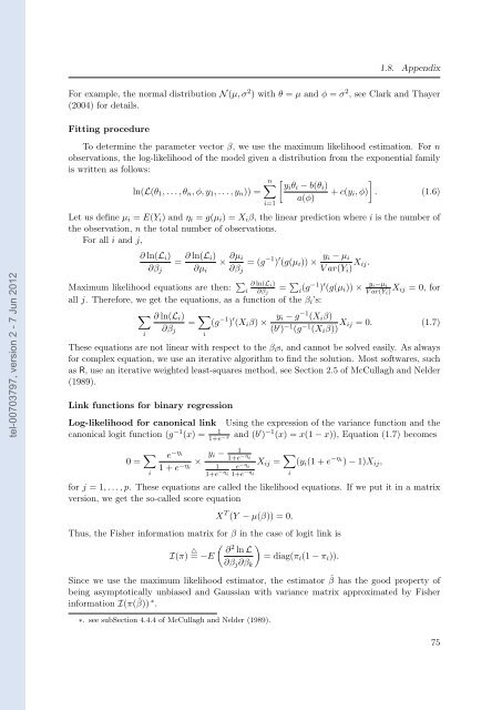
To determine the parameter vector β, we use the maximum likelihood estimation. For n
observations, the log-likelihood of the model given a distribution from the exponential family
is written as follows:
ln(L(θ1, . . . , θn, φ, y1, . . . , yn)) =
n
yiθi − b(θi)
i=1
a(φ)
+ c(yi, φ) . (1.6)
Let us define µi = E(Yi) and ηi = g(µi) = Xiβ, the linear prediction where i is the number of
the observation, n the total number of observations.
For all i and j,
∂ ln(Li)
=
∂βj
∂ ln(Li)
×
∂µi
∂µi
∂βj
Maximum likelihood equations are then: ∂ ln(Li)
i = ∂βj
all j. Therefore, we get the equations, as a function of the βi’s:
∂ ln(Li)
=
∂βj
i
i
= (g −1 ) ′ (g(µi)) × yi − µi
V ar(Yi) Xij.
i (g−1 ) ′ (g(µi)) × yi−µi
V ar(Yi) Xij = 0, for
(g −1 ) ′ (Xiβ) × yi − g−1 (Xiβ)
(b ′ ) −1 (g−1 (Xiβ)) Xij = 0. (1.7)
These equations are not linear with respect to the βis, and cannot be solved easily. As always
for complex equation, we use an iterative algorithm to find the solution. Most softwares, such
as R, use an iterative weighted least-squares method, see Section 2.5 of McCullagh and Nelder
(1989).
Link functions for binary regression
Log-likelihood for canonical link Using the expression of the variance function and the
canonical logit function (g −1 (x) = 1
1+e −x and (b ′ ) −1 (x) = x(1 − x)), Equation (1.7) becomes
0 = e−ηi 1 + e−ηi × yi − 1
1
i
1+e−ηi 1+e−η e
i
−ηi 1+e−ηi Xij =
(yi(1 + e −ηi ) − 1)Xij,
for j = 1, . . . , p. These equations are called the likelihood equations. If we put it in a matrix
version, we get the so-called score equation
X T (Y − µ(β)) = 0.
Thus, the Fisher information matrix for β in the case of logit link is
I(π) △
∂2 ln L
= −E
= diag(πi(1 − πi)).
∂βj∂βk
Since we use the maximum likelihood estimator, the estimator ˆ β has the good property of
being asymptotically unbiased and Gaussian with variance matrix approximated by Fisher
information I(π( ˆ β)) ∗ .
∗. see subSection 4.4.4 of McCullagh and Nelder (1989).
i
75