Etude des marchés d'assurance non-vie à l'aide d'équilibres de ...

tel-00703797, version 2 - 7 Jun 2012
Chapitre 1. Sur la nécessité d’un modèle de marché
The parameters θ, called thresholds, have a special interpretation since they link the
response variable Z with a latent variable U by the equation Z = dk ⇔ θk−1 < U ≤ θk.
Hence, the trick to go from a Bernoulli model to a polytomous model is to have different
ordered intercept coefficients θk’s for the different categorical values.
As in Dionne et al. (2001), our choice goes to the ordered logit model for its simplicity.
So, Z is modelled by the following equation
−1
P (Zi ≤ j/Xi, Yi) = g θj + X T i β + Yiγ +
E(Y |Xi)δ ,
for individual i and deductible j, with g −1 the logistic distribution function ∗ and Xi exogeneous
explanatory variables as opposed to endegeneous variables Yi. The parameters of this
model equation are the regression coefficients β and γ and the threshold parameter θk’s.
1.5.3 Application on the large dataset of Subsection 1.3.2
We want to test for evidence of adverse selection on the full comprehensive (FC) coverage
product. So, we study in this subsection only the three datasets relative to that coverage.
First, we model the claim number, and then we test for the asymmetry of information.
Modelling the claim number
Modelling count data in the generalized linear model framework can be done by choosing
an appropriate distribution: the Poisson and overdispersed Poisson distribution, cf. Table
1.1, where the canonical link function is the logarithm. Since for a Poisson distribution P(λ),
P (Y = 0) = e −λ , the GLM Poisson consists in assuming
E(Y/ xi) = e xT i β ⇔ − log P (Y = 0/ xi) = x T i β.
where xi denotes the covariates. In practice, this models suffers a subparametrization of the
Poisson distribution, one single parameter.
One could think that the Negative binomial in an extended GLM † framework will tackle
this issue, but in practice the mass in zero is so high, that both Poisson and negative binomial
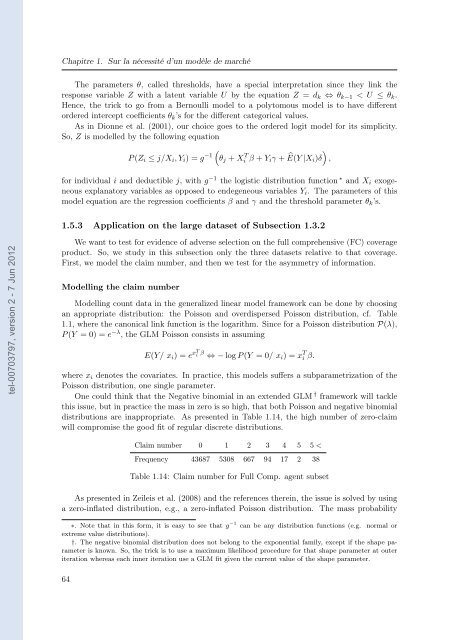
distributions are inappropriate. As presented in Table 1.14, the high number of zero-claim
will compromise the good fit of regular discrete distributions.
Claim number 0 1 2 3 4 5 5 <
Frequency 43687 5308 667 94 17 2 38
Table 1.14: Claim number for Full Comp. agent subset
As presented in Zeileis et al. (2008) and the references therein, the issue is solved by using
a zero-inflated distribution, e.g., a zero-inflated Poisson distribution. The mass probability
∗. Note that in this form, it is easy to see that g −1 can be any distribution functions (e.g. normal or
extreme value distributions).
†. The negative binomial distribution does not belong to the exponential family, except if the shape parameter
is known. So, the trick is to use a maximum likelihood procedure for that shape parameter at outer
iteration whereas each inner iteration use a GLM fit given the current value of the shape parameter.
64