Etude des marchés d'assurance non-vie à l'aide d'équilibres de ...

tel-00703797, version 2 - 7 Jun 2012
Chapitre 2. Theorie des jeux et cycles de marché
since strategic environments (action sets) evolve over a time, the action set is not finite and
stochastic pertubations complete the picture.
We choose a repeated game but with infinite action space, such that at each period,
insurers set new premiums depending on past observed losses. A generalized Nash equilibrium
is computed at each period. Our repeated game does not enter the framework of dynamic
games as presented in Basar and Olsder (1999), but it shares some properties of Markov games
and classical repeated games.
2.4.2 Deriving a dynamic model
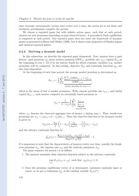
In this subsection, we describe the repeated game framework. Now, insurers have a past
history: past premium x ⋆ j,t gross written premium GWPj,t, portfolio size nj,t, capital Kj,t at
the beginning of year t. Let d be the history depth for which economic variables (e.g. market
premium) will be computed. In this setting, objective Oj,t and constraint functions gj,t are
also time-dependent.
At the beginning of each time period, the average market premium is determined as
¯mt−1 = 1
d
d
u=1
N j=1 GWPj,t−u × x⋆ j,t−u
GWP.,t−u
,
market premium for year t−u
which is the mean of last d market premiums. With current portfolio size nj,t−1 and initial
capital Kj,t−1, each insurer computes its actuarially based premium as
1 1
āj,t =
1 − ej,t d
d sj,t−u
nj,t−u
,
avg ind loss
where sj,t denotes the observed aggregate loss of insurer j during year t. Thus, break-even
premiums are πj,t = ωjāj,t + (1 − ωj) ¯mt−1. Thus, the objective function in the dynamic model
is given by
Oj,t(x) = nj,t
n
and the solvency constraint function by
u=1
xj
1 − βj,t − 1 (xj − πj,t) ,
mj(x)
g 1 j,t(xj) = Kj,t + nj,t(xj − πj,t)(1 − ej,t)
k995σ(Y ) √ nj,t
It is important to note that the characteristics of insurers evolve over time, notably the breakeven
premium πj,t, the expense rate ej,t and the sentivity parameter βj,t.
The game sequence for period t is as follows
116
1. The insurers maximize their objective function subject to the solvency constraint
sup
xj,t
− 1.
Oj,t(xj,t, x−j,t) such that gj,t(xj,t) ≥ 0.
2. Once the premium equilibrium vector x ⋆ t is determined, customers randomly lapse or
renew, so we get a realization n ⋆ j,t of the random variable Nj,t(x ⋆ ).