Etude des marchés d'assurance non-vie à l'aide d'équilibres de ...

tel-00703797, version 2 - 7 Jun 2012
2.3. Refinements of the one-period model
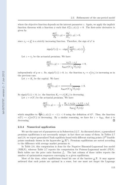
where the objective function depends on the interest parameter z. Again, we apply the implicit
function theorem with a function φ such that G j x(z, φ(z)) = 0. The first-order derivative is
given by
∂G j x
∂y (z, y) = ∂g1 j
(z, y) > 0,
∂xj
since xj ↦→ ˜g 1 j is a strictly increasing function. Therefore, the sign of φ′ is
sign φ ′ (z) = −sign
Let z = πj be the actuarial premium. We have
∂G j x
∂z
∂G j x
(z, φ(z))
∂z
nj(1 − ej)
(z, y) = −
k995σ(Y ) ˆNj(x j < 0,
y)
independently of y or z. So, sign(φ ′ (z)) > 0, i.e. the function πj ↦→ x ⋆ j (πj) is increasing as in
the previous case.
Let z = Kj be the capital. We have
∂G j x
(z, y) =
∂z
1
k995σ(Y ) ˆNj(x j > 0.
y)
So sign(φ ′ (z)) < 0, i.e. the function Kj ↦→ x ⋆ j (Kj) is decreasing.
Let z = σ(Y ) be the actuarial premium. We have
∂G j x 1
(z, y) = −
∂z
z2 × Kj + nj(y − πj)(1 − ej)
k995
ˆNj(x j y)
which simplifies to ∂Gj x
∂z (z, φ(z)) = −1/z < 0 using the definition of Gj . Thus, the function
σ(Y ) ↦→ x ⋆ j (σ(Y )) is decreasing. By a similar reasoning, we have for z = k995, that φ is
decreasing.
2.3.4 Numerical application
We use the same set of parameters as in Subsection 2.2.7. As discussed above, a generalized
premium equilibrium is not necessarily unique: in fact there are many of them. In Tables 2.7
and 2.8, we report generalized Nash equilibria found with different starting points (2 10 feasible
points randomly drawn in the hypercube [x, x] I ). Premium equilibrium are sorted according
to the difference with average market premium ¯m.
In Table 2.8, this computation is done for the Negative Binomial-Lognormal loss model
(NBLN), whereas Table 2.7 reports the computation for Poisson-Lognormal model (PLN).
Both tables use the price ratio function ¯ fj. The last column of those tables reports the
number of optimization sequences converging to a given equilibrium.
Most of the time, other equilibriums found hit one of the barriers x, x. It may appear
awkward that such points are optimal in a sense, but one must not forget the Lagrange
.
,
113