Etude des marchés d'assurance non-vie à l'aide d'équilibres de ...

tel-00703797, version 2 - 7 Jun 2012
Chapitre 2. Theorie des jeux et cycles de marché
Non-uniqueness issues
Uniqueness of a generalized Nash equilibrium is not guaranteed in general. Furthermore,
there is no particular reason for a player to choose a certain Nash equilibrium rather than
another one. Rosen (1965) studied uniqueness of such an equilibrium in a jointly convex
game (i.e. where objective functions are convex and the constraint function is common and
convex). To deal with non-uniqueness, he studies a subset of generalized Nash equilibrium,
where Lagrange multipliers resulting from the Karush-Kuhn-Tucker (KKT) conditions are
normalized. Such a normalized equilibrium is unique given a scale of the Lagrange multiplier
when the constraint function verifies additional assumptions. Other authors such as von
Heusinger and Kanzow (2009) or Facchinei et al. (2007) define normalized equilibrium when
Lagrange multipliers are set equal.
Another way is to look for generalized Nash equilibria having some specific properties, such
as Pareto optimality. The selection of the equilibrium is particularly developed for games with
finite action sets. In that setting, one can also use a mixed strategy, by playing ramdomly one
among many equilibrium strategies.
Parameter sensitivity
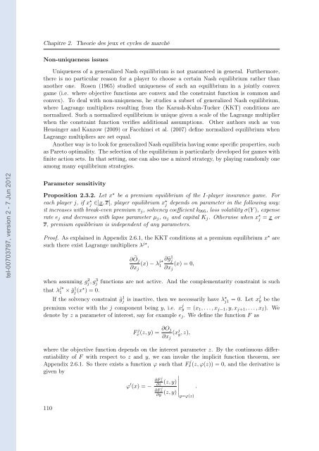
Proposition 2.3.2. Let x⋆ be a premium equilibrium of the I-player insurance game. For
each player j, if x⋆ j ∈]x, x[, player equilibrium x⋆j depends on parameter in the following way:
it increases with break-even premium πj, solvency coefficient k995, loss volatility σ(Y ), expense
rate ej and decreases with lapse parameter µj, αj and capital Kj. Otherwise when x⋆ j = x or
x, premium equilibrium is independent of any parameters.
Proof. As explained in Appendix 2.6.1, the KKT conditions at a premium equilibrium x ⋆ are
such there exist Lagrange multipliers λ j⋆ ,
∂ Oj
∂xj
(x) − λ j⋆ ∂˜g
1
1 j
(x) = 0,
∂xj
when assuming g2 j , g3 j functions are not active. And the complementarity constraint is such
that λ j⋆
1 × ˜g1 j (x⋆ ) = 0.
If the solvency constraint ˜g 1 j is inactive, then we necessarily have λ⋆ j1 = 0. Let xjy be the
premium vector with the j component being y, i.e. x j y = (x1, . . . , xj−1, y, xj+1, . . . , xI). We
denote by z a parameter of interest, say for example ej. We define the function F as
F j x(z, y) = ∂Oj
(x
∂xj
j y, z),
where the objective function depends on the interest parameter z. By the continuous differentiability
of F with respect to z and y, we can invoke the implicit function theorem, see
Appendix 2.6.1. So there exists a function ϕ such that F j x(z, ϕ(z)) = 0, and the derivative is
given by
∂F j
x (z, y)
110
ϕ ′ (x) = −
∂z
∂F j x
∂y
(z, y)
y=ϕ(z)
.