

Etude des marchés d'assurance non-vie à l'aide d'équilibres de ...
Etude des marchés d'assurance non-vie à l'aide d'équilibres de ...
Etude des marchés d'assurance non-vie à l'aide d'équilibres de ...

You also want an ePaper? Increase the reach of your titles
YUMPU automatically turns print PDFs into web optimized ePapers that Google loves.
tel-00703797, version 2 - 7 Jun 2012<br />
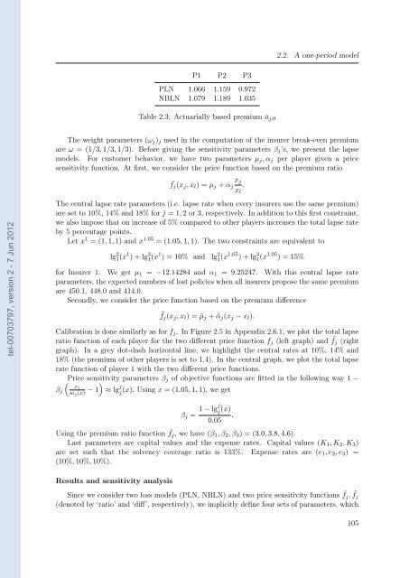
P1 P2 P3<br />
PLN 1.066 1.159 0.972<br />
NBLN 1.079 1.189 1.035<br />
Table 2.3: Actuarially based premium āj,0<br />
2.2. A one-period mo<strong>de</strong>l<br />
The weight parameters (ωj)j used in the computation of the insurer break-even premium<br />
are ω = (1/3, 1/3, 1/3). Before giving the sensitivity parameters βj’s, we present the lapse<br />
mo<strong>de</strong>ls. For customer behavior, we have two parameters µj, αj per player given a price<br />
sensitivity function. At first, we consi<strong>de</strong>r the price function based on the premium ratio<br />
¯fj(xj, xl) = µj + αj<br />
The central lapse rate parameters (i.e. lapse rate when every insurers use the same premium)<br />
are set to 10%, 14% and 18% for j = 1, 2 or 3, respectively. In addition to this first constraint,<br />
we also impose that on increase of 5% compared to other players increases the total lapse rate<br />
by 5 percentage points.<br />
Let x 1 = (1, 1, 1) and x 1.05 = (1.05, 1, 1). The two constraints are equivalent to<br />
lg 2 1(x 1 ) + lg 3 1(x 1 ) = 10% and lg 2 1(x 1.05 ) + lg 3 1(x 1.05 ) = 15%<br />
for Insurer 1. We get µ1 = −12.14284 and α1 = 9.25247. With this central lapse rate<br />
parameters, the expected numbers of lost policies when all insurers propose the same premium<br />
are 450.1, 448.0 and 414.0.<br />
Secondly, we consi<strong>de</strong>r the price function based on the premium difference<br />
xj<br />
xl<br />
˜fj(xj, xl) = ˜µj + ˜αj(xj − xl).<br />
Calibration is done similarly as for fj. In Figure 2.5 in Appendix 2.6.1, we plot the total lapse<br />
ratio function of each player for the two different price function fj (left graph) and ˜ fj (right<br />
graph). In a grey dot-dash horizontal line, we highlight the central rates at 10%, 14% and<br />
18% (the premium of other players is set to 1.4). In the central graph, we plot the total lapse<br />
rate function of player 1 with the two different price functions.<br />
Price sensitivity parameters βj <br />
of objective functions are fitted in the following way 1 −<br />
xj<br />
βj mj(x) − 1 ≈ lg j<br />
j (x). Using x = (1.05, 1, 1), we get<br />
1 − lgj j<br />
βj = (x)<br />
.<br />
0.05<br />
Using the premium ratio function ¯ fj, we have (β1, β2, β3) = (3.0, 3.8, 4.6).<br />
Last parameters are capital values and the expense rates. Capital values (K1, K2, K3)<br />
are set such that the solvency coverage ratio is 133%. Expense rates are (e1, e2, e3) =<br />
(10%, 10%, 10%).<br />
Results and sensitivity analysis<br />
Since we consi<strong>de</strong>r two loss mo<strong>de</strong>ls (PLN, NBLN) and two price sensitivity functions ¯ fj, ˜ fj<br />
(<strong>de</strong>noted by ‘ratio’ and ‘diff’, respectively), we implicitly <strong>de</strong>fine four sets of parameters, which<br />
.<br />
105


