Three-Dimensional Instabilities and Transition in Pulsatile Stenotic ...

15th Australasian Fluid Mechanics Conference
The University of Sydney, Sydney, Australia
13-17 December 2004
Abstract
Three-Dimensional Instabilities and Transition in Pulsatile Stenotic Flows
A straight tube with a smooth axisymmetric constriction is an
idealised representation of a stenosed artery. We examine the
three-dimensional instability of steady flow plus an oscillatory
component in a tube with a smooth 75% stenosis using both
linear stability analysis and direct numerical simulation. These
flows become unstable through a subcritical period-doubling bifurcation
involving alternating tilting of the vortex rings that are
ejected from the throat with each pulse. These tilted vortex rings
rapidly break down through a self-induction mechanism within
the confines of the tube. While the linear instability modes for
pulsatile flow have maximum energy well downstream of the
stenosis, we have established using direct numerical simulation
that breakdown can gradually propagate upstream until it occurs
within a few tube diameters of the constriction, in agreement
with previous experimental observations.
Introduction
Atherosclerosis, the formation of plaques within the arterial
wall, continues to be a major cause of death in the developed
world. The associated narrowing, or stenosis, of the artery can
lead to potential significant restriction of blood flow to downstream
vessels. Related to this condition is the potential of
plaque ruptures and thrombosis formation leading to particles
becoming lodged in smaller vessels possibly inducing myocardinal
infarction or stroke.
This association of arterial disease with flow related mechanisms,
such as wall shear stress variation, has motivated the
study of steady and pulsatile flow within both idealised axisymmetric
and anatomically correct arterial model stenoses [4]. Under
standard physiological flow conditions most arterial flows
are usually considered to be laminar, although typically separated
and unsteady. However in the case of a stenotic flow the
increase in local Reynolds number at a contraction can lead to
transitional flow associated with the early stages of turbulence.
The occurrence of turbulence-like flow phenomena makes the
numerical simulation of these flows particularly challenging especially
when considering the large range of parameters required
to describe both the geometrical and flow features.
In the current work, we turn our attention to the stability of
pulsatile flows in an axisymmetric stenotic tube. The approach
adopted is to analyse the global linear stability of the axisymmetric
flows to arbitrary three-dimensional perturbations. As
the problem has rotational symmetry about the cylindrical axis,
it is natural to use Fourier decomposition in the azimuth direction
in order to break the general three-dimensional linear stability
problem into a set of two-dimensional ones, dramatically
reducing the size of each individual problem. Once we have the
most unstable mode, we then use full three-dimensional direct
numerical simulation (DNS) in order to examine the evolution
of their instability modes, onset of turbulence, and nonlinear
dynamics.
H. M. Blackburn 1 and S. J. Sherwin 2
1 CSIRO Manufacturing and Infrastructure Technology,
Highett, Vic., 3190, AUSTRALIA
2 Department of Aeronautics, Imperial College London,
South Kensington Campus, London, SW7 2AZ, UK
D
r
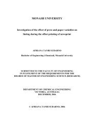
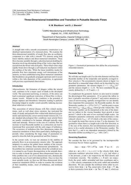
Figure 1: Geometrical parameters that define the axisymmetric
sinusoidal stenosis.
Parameter Space
We will take our length scale D as the tube diameter and base the
Reynolds number on the temporally and spatially averaged inflow
velocity ū. The axisymmetric stenosis shown in figure 1 is
described by a sinusoidal shape which can be described by two
geometric parameters: the stenosis degree S = 1 −(Dmin/D) 2
and the stenosis length λ = L/D. We have considered the geometry
defined by S = 0.75 and λ = 2.
To complement the geometric factors we also need to consider
the physiological flow parameters. If we permit the inflow to
have a pulsatile waveform of period T and restrict attention to
cases of non-reversing, spatially averaged flow we can identify
three important flow parameters: the Reynolds number, Re; the
Womersley number, α = (D 2 π/(2νT)) 1/2 and the peak to mean
flow ratio Upm = Qpeak/Qmean, where Q is the volume flux. The
Womersley number can be interpreted as the ratio of the diameter
(or radius) to the viscous boundary layer growth in time
period T which is the ratio of two sectional length scales. An
alternative parameter commonly used in fluid mechanics is the
reduced velocity Ured = ūT/D which is the ratio of the convective
length the mean flow moves in time T to the diameter. For
geometries where there is a length scale in the flow direction, as
is the case of the stenosis, this non-dimensional parameter can
prove to be a useful alternative to the Womersley number. We
note that Ured and α are dependent parameters related by the
Reynolds number according to Ured = πRe/(2α 2 ).
Governing Equations
We consider the flow to be governed by the incompressible
Newtonian Navier–Stokes equations
L
D min
∂tu = −A(u) − ∇P+ν∇ 2 u, with ∇ · u = 0, (1)
where u = u(z,r,θ,t) = (u,v,w)(t) is the velocity field, A(u)
represents nonlinear advection terms, P = p/ρ, and where p
is the pressure, ρ and ν are respectively the fluid density and
ν kinematic viscosity. The variables z, r, θ and t are respectively
the axial, radial, azimuthal and time coordinates and u,
v, w the velocity components in the axial, radial and azimuthal
directions. We can consider the nonlinear terms either in convective
form A(u) = u · ∇u, conservative form A(u) = ∇ · uu,
or skew-symmetric form A(u) = (u · ∇u+∇·uu)/2, which are
z

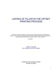
Figure 2: Spectral element outlines of computational mesh, dimensions given in terms of tube diameter D. Panel (a) shows elements
for the first mesh with an outflow at 45D. Panel (b) shows a close-up of the throat, with curved element edges.
all equivalent in a continuum setting. Equation (1) is subject to
no-slip boundary conditions at the walls, a prescribed velocity
at the inflow (steady or periodic), conditions of zero pressure
and zero outward normal derivatives of velocity at the outflow
and consistent regularity boundary conditions at the axis as explained
in [7].
Taking the pressure to represent the solution of a Poisson equation
that has the divergence of the advection terms as forcing,
we can consider the Navier–Stokes equations in symbolic form
as
∂tu = −(I − ∇∇ −2 ∇·)A(u)+ν∇ 2 u = N(u)+L(u) (2)
where the nonlinear operator N contains contributions from
both pressure and advection terms, while the linear operator L
corresponds to viscous diffusion.
When analysing the linear stability of a flow in terms of its normal
modes, we decompose the velocity u into a base flow U and
perturbation flow u ′ : u = U+u ′ , and examine the stability of
the perturbation linearised about the base flow. In this decomposition,
the original nonlinear advection terms are replaced
with their linearised equivalent (here for the convective form)
∂UA(u ′ ) = U · ∇u ′ + u ′ ·∇U and in symbolic form we write
∂tu ′ = ∂UN(u ′ )+L(u ′ ) (3)
for the evolution of the linear perturbation. If the base flow is
T -periodic in time, ∂UN is linear time-periodic, and
u ′ Z
t0+T
(t0 + T) = exp (∂UN+L)dt u ′ (t0). (4)
t0
The eigenpairs of this Floquet problem are {µ, ũ(t0)} where
µ is a Floquet multiplier and ũ(t0) is the T -periodic Floquet
eigenfunction, evaluated at phase t0. The equivalent to the
eigenvalues γ of the time-invariant case are the Floquet exponents
σ, related to the multipliers by µ = expσT . In general,
the Floquet multipliers/exponents and eigenfunctions occur in
complex-conjugate pairs.
Since the geometry is axisymmetric, the velocity must be 2πperiodic
in θ and can be projected exactly onto a set of two-dimensional
complex Fourier modes by
ûk(z,r,t) = 1
2π
Z 2π
0
u(z,r,θ,t)exp(−ikθ)dθ (5)
where k is an integer wavenumber. The Fourier-transformed
equations of motion and axial boundary conditions for the velocity
and pressure (and their perturbations) in cylindrical coordinates
are described in detail in [5, 7]. Our base flows are
(b)
(a)
both axisymmetric/two-dimensional, i.e. Uk = 0, k = 0, and
two-component, i.e. U ≡ (U,V,0). In the numerical stability
analysis we take advantage of linearity, which decouples the
stability problem for each û ′ k .
Numerical Methods
For time evolution of both the full and linearised Navier–
Stokes equations, we relied on standard (nodal-Gauss–Lobatto–
Legendre) spectral elements in (z, r) and Fourier expansions if
required in the azimuthal θ-direction. This spatial discretisation
was coupled with a second-order-time velocity correction timeintegration
scheme. The development of this numerical method
for DNS has been described in detail in [7]. The application
of the method to linearised Navier–Stokes evolution, including
appropriate boundary conditions, has also previously been described
in [5].
The computational mesh used in the calculations is shown in
figure 2. The domain consists of 743 elemental regions. In each
element, two-dimensional mapped tensor-product Lagrangeinterpolant
shape functions based on the Gauss–Lobatto–
Legendre nodes were applied. At P = 7 this elemental discretisation
corresponds to approximately 38 000 local degrees
of freedom in each meridional semiplane. The domain extended
5D upstream and 45D downstream of the throat. As shown in
figure 2 (b) a fine radial mesh spacing was adopted in the region
of the stenosis where two layers each of 5% of the local radius
were applied. At z/D ≈ 7 the radial mesh spacing was coarsened
to allow a uniform axial spacing of 0.5D to be applied to
the outflow. The mesh was refined until both the axisymmetric
base flows and Floquet multipliers converged to four significant
figures. Typically this also gives enough mesh refinement in the
meridional semi-plane for non-axisymmetric DNS as well, with
the number of planes of data in azimuth selected to provide a
three-order or better reduction in kinetic energy from azimuthal
mode 1 to the highest mode.
The numerical methods employed for stability analysis of both
steady and pulsatile flow follow those outlined in [10], and previously
described and used in other works [3, 5, 6]. The analysis
is based on a Krylov-subspace iteration of successive finite
increments of (initially random) perturbations through the operator
of (4) using an Arnoldi method to extract the dominant
eigenpairs of the exponential operators in the equations. The
data used to supply the T -periodic base flow are approximated
through Fourier-series reconstruction from a limited number
(typically 256) of time-slices obtained from two-dimensional
DNS.

(a)
(b)
(c)
(d)
0 5 10 15
0 5 10 15
z/D
15 20 25 30
15 20 25 30
z/D
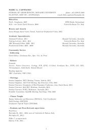
Figure 3: The base flow and the leading eigenmode for one phase in the flow cycle for the unstable pulsatile flow at Re = 400, Ured = 2.5,
on a vertical centreplane. Panels (a, c) show contours of axial velocity of the base flow, while (b, d) show contours of axial velocity of
the eigenmode.
Figure 4: Growth to saturation of the pulsatile inlet flow solution
at Ured = 2.5, Re = 400, approximately 3% above Rec, represented
by kinetic energies in azimuthal Fourier modes, with
Nk = 16. An initial exponential growth phase (indicated by the
dotted line) is followed by faster than exponential growth near
t/T ∼ 35, an initial nonlinear saturation at t/T ≈ 40, then a final
slow growth to an asymptotic state, reached at t/T ∼ 250.
Results
Floquet analysis was carried out at Upm = 1.75 and for three
values of reduced velocity: Ured = 2.5, 5, and 7.5, i.e. successively
longer dimensionless base flow periods. The corresponding
critical Reynolds numbers were found to be Rec = 389,
417 and 500. In all three cases, the instability arose through
a period-doubling bifurcation in the k = 1 azimuthal Fourier
mode. The shape and location of the Floquet instability mode
for Ured = 2.5, Re = 400 is shown in figure 3, where it is compared
to the base flow at the same instant in time. The alternating
sign of the Floquet mode growing on successive base flow
pulses for a streamwise traverse at any fixed radius is related to
the period-doubling nature of the instability. The perturbation
exerts alternating tilting moments on the vortex rings associated
with each pulse of the base flow.
Following the stability analysis, full three-dimensional DNS of
the instability at Ured = 2.5, Re = 400 was initiated by perturbing
the base flow with a small amount of the leading Flo-
quet eigenmode and evolving in time. The time-evolution of
energies in the azimuthal modes is shown in figure 4. After a
brief equilibration, there is an exponential growth phase in the
non-axisymmetric components, lasting until t/T ≈ 35, following
which the perturbation grows faster than exponentially with
time before an initial saturation at t/T ≈ 40, signalling that the
bifurcation is subcritical. Then there is an extended slow change
until an asymptotic state is approached at t/T ∼ 250.
The evolution of the flow through time is illustrated by the instantaneous
isosurfaces shown in figure 5. The first set of panels,
in figure 5 (a), shows the flow state after the initial saturation
at t/T = 40. In the side view, the tilting of the third vortex
ring in the view can be seen, while the fourth and fifth rings in
the view are further advanced in their breakdowns to a packet of
Λ-vortices. In figure 5 (b) we see two instances in time leading
to the asymptotic state: the slow final growth seen in figure 4 is
associated with an upstream movement of the vortex ring breakdown.
At t/T = 280, the flow still has the symmetry of the Floquet
mode, but at that point a small random symmetry-breaking
perturbation was added to the first azimuthal mode, and the flow
further evolved in time, leading to another asymptotic, but now
asymmetric state seen in figure 5 (c). At large length and time
scales, the flow still has a period-doubling nature, indicating
that this is a robust feature.
Discussion
The experimental results of [1, 2, 9] provide a basis for comparison
to our DNS results. These were performed at a higher value
of Ured, but similar Reynolds number (Re ≈ 600) and peak-tomean
flow ratio (Upm ≈ 1.7).
In [2] it is stated that ‘turbulence was found only for the 75%
stenosis and was created only during part of the cycle’, whereas
in [1] these fluctuations, which are strongest for 2.5 < z/D 6,
are characterised as non-turbulent owing to the presence in the
conditional velocity spectra of a band of dominant frequencies
associated with ‘vortex shedding and a turbulent front’. These
findings are in quite good agreement with the dye-front flow
visualisation and interpretation provided by [9]. For the 75%
stenosis, they found four post-stenotic zones: Zone I, reaching
to z/D = 3, is called the ‘stable jet region’, although some indication
of (apparently axisymmetric) wavy structure can be ob-

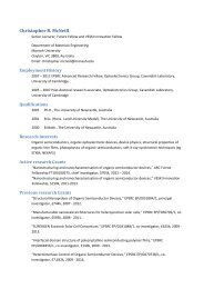
top
t = 40T
side
t = 132T
t = 280T
t = 300.625T
(a)
(b)
(c)
Figure 5: Visualisations for the DNS of pulsatile flow at Ured = 2.5, Re = 400. Isosurfaces are extracted using the λ2 criterion [8]. (a)
top and side views of the flow just after the initial saturation seen at t/T = 40 in figure 4. (b) Two visualisations at later times in the
progression to the asymptotic state. Note the upstream movement of breakdown. (c) A detail perspective view of the breakdown of
vortex rings in the cycle following t = 300T . Downstream of the stenosis, the first group of structures shows a ring deforming during
the final stages of the tilting process, while the second group shows the decaying breakdown of the previous ring.
served on the jet front in this region; Zone II, 3 < z/D 4.5 is
called the ‘transition region’, where the waves become larger;
in Zone III, the ‘turbulent region’, 4.5 < z/D 7.5, the front
rapidly distorts; Zone IV, z/D > 7.5 is labelled ‘relaminarization’.
These experimental results are thus in reasonable agreement
with the kind of asymptotic behaviour we have observed in
DNS, as can be seen in figure 5 (b, c): a rapid distortion of a vortex
ring becoming evident a few diameters downstream of the
stenosis, leading to a highly unsteady/transitional breakdown at
z/D ∼ 6, following which relaminarisation takes place further
downstream.
Conclusions
Floquet analysis of three axisymmetric pulsatile flows shows
that they become three-dimensionally unstable through perioddoubling
bifurcations involving alternating tilting of the vortex
rings that are ejected from the stenosis during each pulse cycle.
Direct numerical simulation shows that the instability evolves
to vortex ring breakdown, which moves progressively upstream
until it occurs a comparatively few tube diameters downstream
of the stenosis. As the bifurcations are subcritical, hysteretic
effects can be expected with respect to changes in Reynolds
number, reduced velocity, or peak-to-mean pulsatility near the
onset of three-dimensionality. The breakdowns are energetic
turbulent events, and will lead to regions of high temporal and
spatial gradients of wall shear stress where they occur. For the
Reynolds numbers studied here, the flow relaminarises further
downstream, and will eventually recover the conditions of the
pulsatile inflow. These findings are in good agreement with
available experimental results.
Acknowledgements
This work was supported by the Australian Partnership for Advanced
Computing, the Royal Academy of Engineering, and the
UK Engineering and Physical Sciences Research Council.
References
[1] Ahmed SA. An experimental investigation of pulsatile
flow through a smooth constriction. Exptl Thermal &
Fluid Sci, 17: 309–318, 1998
[2] Ahmed SA & Giddens DP. Pulsatile poststenotic flow
studies with laser Doppler anemometry. J Biomechanics,
17(9): 695–705, 1984
[3] Barkley D & Henderson RD. Three-dimensional Floquet
stability analysis of the wake of a circular cylinder. J Fluid
Mech, 322: 215–241, 1996
[4] Berger SA & Jou LD. Flows in stenotic vessels. Annu Rev
Fluid Mech, 32: 347–384, 2000
[5] Blackburn HM. Three-dimensional instability and state
selection in an oscillatory axisymmetric swirling flow.
Phys Fluids, 14(11): 3983–3996, 2002
[6] Blackburn HM & Lopez JM. The onset of threedimensional
standing and modulated travelling waves in
a periodically driven cavity flow. J Fluid Mech, 497: 289–
317, 2003
[7] Blackburn HM & Sherwin SJ. Formulation of a Galerkin
spectral element–Fourier method for three-dimensional
incompressible flows in cylindrical geometries. J Comput
Phys, 197(2): 759–778, 2004
[8] Jeong J & Hussain F. On the identification of a vortex.
J Fluid Mech, 285: 69–94, 1995
[9] Ojha M, Cobbold RSC, Johnston KW & Hummel RL.
Pulsatile flow through constricted tubes: An experimental
investigation using photochromic tracer methods. J Fluid
Mech, 203: 173–197, 1989
[10] Tuckerman LS & Barkley D. Bifurcation analysis for
timesteppers. In E Doedel & LS Tuckerman, editors,
Numerical Methods for Bifurcation Problems and Large-
Scale Dynamical Systems, 453–566. Springer, 2000