ENTANGLEMENT OF GAUSSIAN STATES Gerardo Adesso

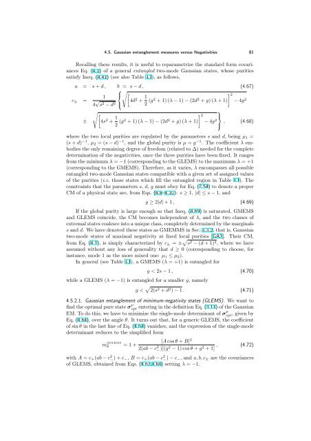
4.5. Gaussian entanglement measures versus Negativities 81
Recalling these results, it is useful to reparametrize the standard form covariances
Eq. (4.1) of a general entangled two-mode Gaussian states, whose purities
satisfy Ineq. (4.41) (see also Table 4.I), as follows,
a = s + d , b = s − d , (4.67)
1
4 √ s2 − d2 ⎧
⎨
4d
⎩
2 + 1
2 (g2 + 1) (λ − 1) − (2d2 2 + g) (λ + 1) − 4g2 ±
4s2 + 1
2 (g2 + 1) (λ − 1) − (2d2 2 + g) (λ + 1) − 4g2 ⎫
⎬
,
⎭
(4.68)
c± =
where the two local purities are regulated by the parameters s and d, being µ1 =
(s + d) −1 , µ2 = (s − d) −1 , and the global purity is µ = g −1 . The coefficient λ embodies
the only remaining degree of freedom (related to ∆) needed for the complete
determination of the negativities, once the three purities have been fixed. It ranges
from the minimum λ = −1 (corresponding to the GLEMS) to the maximum λ = +1
(corresponding to the GMEMS). Therefore, as it varies, λ encompasses all possible
entangled two-mode Gaussian states compatible with a given set of assigned values
of the purities (i.e. those states which fill the entangled region in Table 4.I). The
constraints that the parameters s, d, g must obey for Eq. (2.54) to denote a proper
CM of a physical state are, from Eqs. (4.8–4.10): s ≥ 1, |d| ≤ s − 1, and
g ≥ 2|d| + 1 , (4.69)
If the global purity is large enough so that Ineq. (4.69) is saturated, GMEMS
and GLEMS coincide, the CM becomes independent of λ, and the two classes of
extremal states coalesce into a unique class, completely determined by the marginals
s and d. We have denoted these states as GMEMMS in Sec. 4.3.2, that is, Gaussian
two-mode states of maximal negativity at fixed local purities [GA3]. Their CM,
from Eq. (4.1), is simply characterized by c± = ± s 2 − (d + 1) 2 , where we have
assumed without any loss of generality that d ≥ 0 (corresponding to choose, for
instance, mode 1 as the more mixed one: µ1 ≤ µ2).
In general (see Table 4.I), a GMEMS (λ = +1) is entangled for
g < 2s − 1 , (4.70)
while a GLEMS (λ = −1) is entangled for a smaller g, namely
g < 2(s 2 + d 2 ) − 1 . (4.71)
4.5.2.1. Gaussian entanglement of minimum-negativity states (GLEMS). We want to
find the optimal pure state σ p
opt entering in the definition Eq. (3.11) of the Gaussian
EM. To do this, we have to minimize the single-mode determinant of σ p
opt, given by
Eq. (4.64), over the angle θ. It turns out that, for a generic GLEMS, the coefficient
of sin θ in the last line of Eq. (4.64) vanishes, and the expression of the single-mode
determinant reduces to the simplified form
m 2GLEMS [A cos θ + B]
θ = 1 +
2
2(ab − c2 −)[(g2 − 1) cos θ + g2 , (4.72)
+ 1]
with A = c+(ab − c 2 −) + c−, B = c+(ab − c 2 −) − c−, and a, b, c± are the covariances
of GLEMS, obtained from Eqs. (4.67,4.68) setting λ = −1.