ENTANGLEMENT OF GAUSSIAN STATES Gerardo Adesso
ENTANGLEMENT OF GAUSSIAN STATES Gerardo Adesso ENTANGLEMENT OF GAUSSIAN STATES Gerardo Adesso
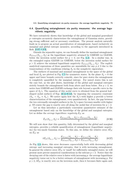
74 4. Two-mode entanglement E E 4 3 2 1 0 0 2 1.5 1 0.5 2 0 0 0.1 0.2 4 SV S3 0.3 (a) (c) 6 0.4 1 0 2 3 SVi 0.1 0 0.2 0.1 0.3 0.4 S3i E 3 2 1 0 0 0.2 0.4 Figure 4.5. Upper and lower bounds on the logarithmic negativity of symmetric Gaussian states as functions of the global and marginal generalized p−entropies, for (a) p = 1 (Von Neumann entropies), (b) p = 2 (linear entropies), (c) p = 3, and (d) p = 4. The blue (yellow) surface represents GMEMS (GLEMS). Notice that for p > 2 GMEMS and GLEMS surfaces intersect along the inversion line (meaning they are equally entangled along that line), and beyond it they interchange their role. The equations of the inversion lines are obtained from Eqs. (4.51–4.53), with the position Sp1 = Sp2 ≡ Sp i . directly from Eq. (2.36) and reads Spi = E 1.5 1 0.5 0 0 1 − gp(1/µi) p − 1 0.1 SL S4 0.6 0.2 (b) (d) 0.8 0.3 0.2 0 0.4 0.2 0.6 0.8 SLi 0 0.1 0.2 S4i . (4.55) We notice prima facie that, with increasing p, the entanglement is more sharply qualified in terms of the global and marginal p−entropies. In fact the region of coexistence between separable and entangled states becomes narrower with higher p. Thus, somehow paradoxically, with increasing p the entropy Sp provides less information about a quantum state, but at the same time it yields a more accurate characterization and quantification of its entanglement. In the limit p → ∞ all the physical states collapse to one point at the origin of the axes in the space of generalized entropies, due to the fact that the measure S∞ is identically zero.
4.4. Quantifying entanglement via purity measures: the average logarithmic negativity 75 4.4. Quantifying entanglement via purity measures: the average logarithmic negativity We have extensively shown that knowledge of the global and marginal generalized p−entropies accurately characterizes the entanglement of Gaussian states, providing strong sufficient and/or necessary conditions. The present analysis naturally leads us to propose an actual quantification of entanglement, based exclusively on marginal and global entropic measures, according to the approach introduced in Refs. [GA2, GA3]. Outside the separable region, we can formally define the maximal entanglement EN max(Sp1,2, Sp) as the logarithmic negativity attained by GMEMS (or GLEMS, below the inversion nodal surface for p > 2, see Fig. 4.3). In a similar way, in the entangled region GLEMS (or GMEMS, below the inversion nodal surface for p > 2) achieve the minimal logarithmic negativity EN min(Sp1,2, Sp). The explicit analytical expressions of these quantities are unavailable for any p = 2 due to the transcendence of the conditions relating Sp to the symplectic eigenvalues. The surfaces of maximal and minimal entanglement in the space of the global and local Sp are plotted in Fig. 4.5 for symmetric states. In the plane Sp = 0 the upper and lower bounds correctly coincide, since for pure states the entanglement is completely quantified by the marginal entropy. For mixed states this is not the case but, as the plot shows, knowledge of the global and marginal entropies strictly bounds the entanglement both from above and from below. For p > 2, we notice how GMEMS and GLEMS exchange their role beyond a specific curve in the space of Sp’s. The equation of this nodal curve is obtained from the general leaf– shaped nodal surfaces of Eqs. (4.51–4.53), by imposing the symmetry constraint (Sp1 = Sp2 ≡ Spi). We notice again how the Sp’s with higher p provide a better characterization of the entanglement, even quantitatively. In fact, the gap between the two extremally entangled surfaces in the Sp’s space becomes smaller with higher p. Of course the gap is exactly zero all along the nodal line of inversion for p > 2. Let us thus introduce a particularly convenient quantitative estimate of the entanglement based only on the knowledge of the global and marginal entropies. Let us define the average logarithmic negativity ĒN as ĒN (Sp1,2, Sp) ≡ EN max(Sp1,2, Sp) + EN min(Sp1,2, Sp) . (4.56) 2 We will now show that this quantity, fully determined by the global and marginal entropies, provides a reliable quantification of entanglement (logarithmic negativity) for two-mode Gaussian states. To this aim, we define the relative error δ ĒN on ĒN as δĒN (Sp1,2, Sp) ≡ EN max(Sp1,2, Sp) − EN min(Sp1,2, Sp) . (4.57) EN max(Sp1,2, Sp) + EN min(Sp1,2, Sp) As Fig. 4.6 shows, this error decreases exponentially both with decreasing global entropy and increasing marginal entropies, that is with increasing entanglement. In general the relative error δ ĒN is ‘small’ for sufficiently entangled states; we will present more precise numerical considerations in the subcase p = 2. Notice that the decaying rate of the relative error is faster with increasing p: the average logarithmic negativity turns out to be a better estimate of entanglement with increasing p. For p > 2, δ ĒN is exactly zero on the inversion node, then it becomes finite again and,
- Page 38 and 39: 24 1. Characterizing entanglement n
- Page 40 and 41: 26 1. Characterizing entanglement p
- Page 43 and 44: CHAPTER 2 Gaussian states: structur
- Page 45 and 46: 2.1. Introduction to continuous var
- Page 47 and 48: 2.2. Mathematical description of Ga
- Page 49 and 50: 2.2. Mathematical description of Ga
- Page 51 and 52: 2.3. Degree of information encoded
- Page 53 and 54: 2.3. Degree of information encoded
- Page 55 and 56: 2.4. Standard forms of Gaussian cov
- Page 57 and 58: 2.4. Standard forms of Gaussian cov
- Page 59 and 60: 2.4. Standard forms of Gaussian cov
- Page 61 and 62: 2.4. Standard forms of Gaussian cov
- Page 63: Part II Bipartite entanglement of G
- Page 66 and 67: 52 3. Characterizing entanglement o
- Page 68 and 69: 54 3. Characterizing entanglement o
- Page 71 and 72: CHAPTER 4 Two-mode entanglement Thi
- Page 73 and 74: 4.2. Entanglement and symplectic ei
- Page 75 and 76: 4.3. Entanglement versus Entropic m
- Page 77 and 78: 1 0.75 0.5 SL1 0.25 0 (a) 4.3. Enta
- Page 79 and 80: 4.3. Entanglement versus Entropic m
- Page 81 and 82: Μ Μ1Μ2 3 2 1 1 4.3. Entanglemen
- Page 83 and 84: 4.3. Entanglement versus Entropic m
- Page 85 and 86: 4.3. Entanglement versus Entropic m
- Page 87: global generalized entropy S3 globa
- Page 91 and 92: 4.4. Quantifying entanglement via p
- Page 93 and 94: 4.5. Gaussian entanglement measures
- Page 95 and 96: 4.5. Gaussian entanglement measures
- Page 97 and 98: 4.5. Gaussian entanglement measures
- Page 99 and 100: 4.5. Gaussian entanglement measures
- Page 101 and 102: Ν p Σopt 1 0.8 0.6 0.4 0.2 0 4.5
- Page 103 and 104: GEF GEF 4 3 2 1 0 4.6. Summary and
- Page 105: 4.6. Summary and further remarks 91
- Page 108 and 109: 94 5. Multimode entanglement under
- Page 110 and 111: 96 5. Multimode entanglement under
- Page 112 and 113: 98 5. Multimode entanglement under
- Page 114 and 115: 100 5. Multimode entanglement under
- Page 116 and 117: 102 5. Multimode entanglement under
- Page 118 and 119: 104 5. Multimode entanglement under
- Page 121: Part III Multipartite entanglement
- Page 124 and 125: 110 6. Gaussian entanglement sharin
- Page 126 and 127: 112 6. Gaussian entanglement sharin
- Page 128 and 129: 114 6. Gaussian entanglement sharin
- Page 130 and 131: 116 6. Gaussian entanglement sharin
- Page 132 and 133: 118 6. Gaussian entanglement sharin
- Page 134 and 135: 120 6. Gaussian entanglement sharin
- Page 136 and 137: 122 7. Tripartite entanglement in t
4.4. Quantifying entanglement via purity measures: the average logarithmic negativity 75<br />
4.4. Quantifying entanglement via purity measures: the average logarithmic<br />
negativity<br />
We have extensively shown that knowledge of the global and marginal generalized<br />
p−entropies accurately characterizes the entanglement of Gaussian states, providing<br />
strong sufficient and/or necessary conditions. The present analysis naturally<br />
leads us to propose an actual quantification of entanglement, based exclusively on<br />
marginal and global entropic measures, according to the approach introduced in<br />
Refs. [GA2, GA3].<br />
Outside the separable region, we can formally define the maximal entanglement<br />
EN max(Sp1,2, Sp) as the logarithmic negativity attained by GMEMS (or GLEMS,<br />
below the inversion nodal surface for p > 2, see Fig. 4.3). In a similar way, in<br />
the entangled region GLEMS (or GMEMS, below the inversion nodal surface for<br />
p > 2) achieve the minimal logarithmic negativity EN min(Sp1,2, Sp). The explicit<br />
analytical expressions of these quantities are unavailable for any p = 2 due to the<br />
transcendence of the conditions relating Sp to the symplectic eigenvalues.<br />
The surfaces of maximal and minimal entanglement in the space of the global<br />
and local Sp are plotted in Fig. 4.5 for symmetric states. In the plane Sp = 0 the<br />
upper and lower bounds correctly coincide, since for pure states the entanglement<br />
is completely quantified by the marginal entropy. For mixed states this is not<br />
the case but, as the plot shows, knowledge of the global and marginal entropies<br />
strictly bounds the entanglement both from above and from below. For p > 2, we<br />
notice how GMEMS and GLEMS exchange their role beyond a specific curve in the<br />
space of Sp’s. The equation of this nodal curve is obtained from the general leaf–<br />
shaped nodal surfaces of Eqs. (4.51–4.53), by imposing the symmetry constraint<br />
(Sp1 = Sp2 ≡ Spi). We notice again how the Sp’s with higher p provide a better<br />
characterization of the entanglement, even quantitatively. In fact, the gap between<br />
the two extremally entangled surfaces in the Sp’s space becomes smaller with higher<br />
p. Of course the gap is exactly zero all along the nodal line of inversion for p > 2.<br />
Let us thus introduce a particularly convenient quantitative estimate of the<br />
entanglement based only on the knowledge of the global and marginal entropies.<br />
Let us define the average logarithmic negativity ĒN as<br />
ĒN (Sp1,2, Sp) ≡ EN max(Sp1,2, Sp) + EN min(Sp1,2, Sp)<br />
. (4.56)<br />
2<br />
We will now show that this quantity, fully determined by the global and marginal<br />
entropies, provides a reliable quantification of entanglement (logarithmic negativity)<br />
for two-mode Gaussian states. To this aim, we define the relative error δ ĒN<br />
on ĒN as<br />
δĒN (Sp1,2, Sp) ≡ EN max(Sp1,2, Sp) − EN min(Sp1,2, Sp)<br />
. (4.57)<br />
EN max(Sp1,2, Sp) + EN min(Sp1,2, Sp)<br />
As Fig. 4.6 shows, this error decreases exponentially both with decreasing global<br />
entropy and increasing marginal entropies, that is with increasing entanglement.<br />
In general the relative error δ ĒN is ‘small’ for sufficiently entangled states; we will<br />
present more precise numerical considerations in the subcase p = 2. Notice that the<br />
decaying rate of the relative error is faster with increasing p: the average logarithmic<br />
negativity turns out to be a better estimate of entanglement with increasing p. For<br />
p > 2, δ ĒN is exactly zero on the inversion node, then it becomes finite again and,


