ENTANGLEMENT OF GAUSSIAN STATES Gerardo Adesso
ENTANGLEMENT OF GAUSSIAN STATES Gerardo Adesso ENTANGLEMENT OF GAUSSIAN STATES Gerardo Adesso
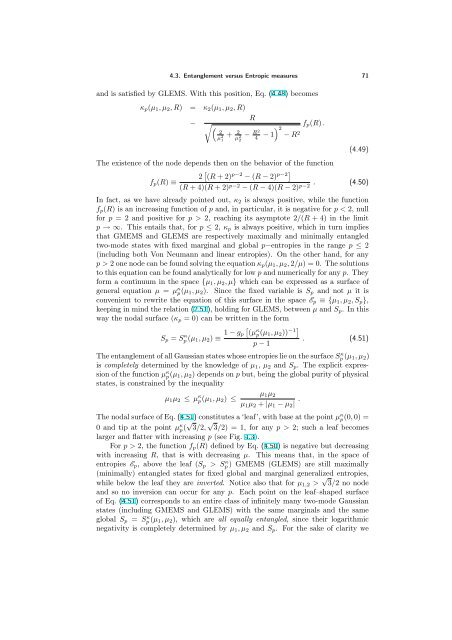
70 4. Two-mode entanglement 0.4 S3 0.2 0 0 0.25 0.5 Μ1 0.75 (a) 1 0.25 0 0.75 0.5 Μ2 Μ2 0.3 0.2 S4 0.1 0 0 0.25 0.5 Μ1 0.75 (b) 1 0.25 0 0.75 0.5 Μ2 Μ2 Figure 4.3. Plot of the nodal surface which solves the equation κp = 0 with κp defined by Eq. (4.48), for (a) p = 3 and (b) p = 4. The entanglement of Gaussian states that lie on the leaf–shaped surfaces is fully quantified in terms of the marginal purities and the global generalized entropy (a) S3 or (b) S4. The equations of the surfaces in the space Ep ≡ {µ1, µ2, Sp} are given by Eqs. (4.51–4.53). Sp for a generic p. Using Maxwell’s relations, we can write κp ≡ ∂(2˜ν2 −) ∂∆ Sp = ∂(2˜ν2 −) ∂∆ R − ∂(2˜ν2 −) ∂R ∆ · ∂Sp/∂∆| R . (4.47) ∂Sp/∂R| ∆ Clearly, for κp > 0 GMEMS and GLEMS retain their usual interpretation, whereas for κp < 0 they exchange their role. On the node κp = 0 GMEMS and GLEMS share the same entanglement, i.e. the entanglement of all Gaussian states at κp = 0 is fully determined by the global and marginal p−entropies alone, and does not depend any more on ∆. Such nodes also exist in the case p ≤ 2 in two limiting instances: in the special case of GMEMMS (states with maximal global purity at fixed marginals) and in the limit of zero marginal purities. We will now show that, besides these two asymptotic behaviors, a nontrivial node appears for all p > 2, implying that on the two sides of the node GMEMS and GLEMS indeed exhibit opposite behaviors. Because of Eq. (4.42), κp can be written in the following form κp = κ2 − R ˜∆ 2 − R 2 with Np and Dp defined by Eq. (4.44) and ˜∆ = −∆ + 2 µ 2 + 1 2 µ 2 2 , κ2 = ˜∆ −1 + , ˜∆ 2 − R2 Np(∆, R) , (4.48) Dp(∆, R) The quantity κp in Eq. (4.48) is a function of p, R, ∆, and of the marginals; since we are looking for the node (where the entanglement is independent of ∆), we can investigate the existence of a nontrivial solution to the equation κp = 0 fixing any value of ∆. Let us choose ∆ = 1 + R 2 /4 that saturates the uncertainty relation
4.3. Entanglement versus Entropic measures 71 and is satisfied by GLEMS. With this position, Eq. (4.48) becomes κp(µ1, µ2, R) = κ2(µ1, µ2, R) − 2 µ 2 1 R + 2 µ 2 − 2 R2 2 4 − 1 − R 2 fp(R) . The existence of the node depends then on the behavior of the function fp(R) ≡ (4.49) 2 (R + 2) p−2 − (R − 2) p−2 (R + 4)(R + 2) p−2 . (4.50) − (R − 4)(R − 2) p−2 In fact, as we have already pointed out, κ2 is always positive, while the function fp(R) is an increasing function of p and, in particular, it is negative for p < 2, null for p = 2 and positive for p > 2, reaching its asymptote 2/(R + 4) in the limit p → ∞. This entails that, for p ≤ 2, κp is always positive, which in turn implies that GMEMS and GLEMS are respectively maximally and minimally entangled two-mode states with fixed marginal and global p−entropies in the range p ≤ 2 (including both Von Neumann and linear entropies). On the other hand, for any p > 2 one node can be found solving the equation κp(µ1, µ2, 2/µ) = 0. The solutions to this equation can be found analytically for low p and numerically for any p. They form a continuum in the space {µ1, µ2, µ} which can be expressed as a surface of general equation µ = µ κ p(µ1, µ2). Since the fixed variable is Sp and not µ it is convenient to rewrite the equation of this surface in the space Ep ≡ {µ1, µ2, Sp}, keeping in mind the relation (2.51), holding for GLEMS, between µ and Sp. In this way the nodal surface (κp = 0) can be written in the form Sp = S κ κ 1 − gp (µ p(µ1, µ2)) p (µ1, µ2) ≡ −1 . (4.51) p − 1 The entanglement of all Gaussian states whose entropies lie on the surface S κ p (µ1, µ2) is completely determined by the knowledge of µ1, µ2 and Sp. The explicit expression of the function µ κ p(µ1, µ2) depends on p but, being the global purity of physical states, is constrained by the inequality µ1µ2 ≤ µ κ p(µ1, µ2) ≤ µ1µ2 µ1µ2 + |µ1 − µ2| . The nodal surface of Eq. (4.51) constitutes a ‘leaf’, with base at the point µ κ p(0, 0) = 0 and tip at the point µ κ p( √ 3/2, √ 3/2) = 1, for any p > 2; such a leaf becomes larger and flatter with increasing p (see Fig. 4.3). For p > 2, the function fp(R) defined by Eq. (4.50) is negative but decreasing with increasing R, that is with decreasing µ. This means that, in the space of entropies Ep, above the leaf (Sp > S κ p ) GMEMS (GLEMS) are still maximally (minimally) entangled states for fixed global and marginal generalized entropies, while below the leaf they are inverted. Notice also that for µ1,2 > √ 3/2 no node and so no inversion can occur for any p. Each point on the leaf–shaped surface of Eq. (4.51) corresponds to an entire class of infinitely many two-mode Gaussian states (including GMEMS and GLEMS) with the same marginals and the same global Sp = S κ p (µ1, µ2), which are all equally entangled, since their logarithmic negativity is completely determined by µ1, µ2 and Sp. For the sake of clarity we
- Page 34 and 35: 20 1. Characterizing entanglement i
- Page 36 and 37: 22 1. Characterizing entanglement e
- Page 38 and 39: 24 1. Characterizing entanglement n
- Page 40 and 41: 26 1. Characterizing entanglement p
- Page 43 and 44: CHAPTER 2 Gaussian states: structur
- Page 45 and 46: 2.1. Introduction to continuous var
- Page 47 and 48: 2.2. Mathematical description of Ga
- Page 49 and 50: 2.2. Mathematical description of Ga
- Page 51 and 52: 2.3. Degree of information encoded
- Page 53 and 54: 2.3. Degree of information encoded
- Page 55 and 56: 2.4. Standard forms of Gaussian cov
- Page 57 and 58: 2.4. Standard forms of Gaussian cov
- Page 59 and 60: 2.4. Standard forms of Gaussian cov
- Page 61 and 62: 2.4. Standard forms of Gaussian cov
- Page 63: Part II Bipartite entanglement of G
- Page 66 and 67: 52 3. Characterizing entanglement o
- Page 68 and 69: 54 3. Characterizing entanglement o
- Page 71 and 72: CHAPTER 4 Two-mode entanglement Thi
- Page 73 and 74: 4.2. Entanglement and symplectic ei
- Page 75 and 76: 4.3. Entanglement versus Entropic m
- Page 77 and 78: 1 0.75 0.5 SL1 0.25 0 (a) 4.3. Enta
- Page 79 and 80: 4.3. Entanglement versus Entropic m
- Page 81 and 82: Μ Μ1Μ2 3 2 1 1 4.3. Entanglemen
- Page 83: 4.3. Entanglement versus Entropic m
- Page 87 and 88: global generalized entropy S3 globa
- Page 89 and 90: 4.4. Quantifying entanglement via p
- Page 91 and 92: 4.4. Quantifying entanglement via p
- Page 93 and 94: 4.5. Gaussian entanglement measures
- Page 95 and 96: 4.5. Gaussian entanglement measures
- Page 97 and 98: 4.5. Gaussian entanglement measures
- Page 99 and 100: 4.5. Gaussian entanglement measures
- Page 101 and 102: Ν p Σopt 1 0.8 0.6 0.4 0.2 0 4.5
- Page 103 and 104: GEF GEF 4 3 2 1 0 4.6. Summary and
- Page 105: 4.6. Summary and further remarks 91
- Page 108 and 109: 94 5. Multimode entanglement under
- Page 110 and 111: 96 5. Multimode entanglement under
- Page 112 and 113: 98 5. Multimode entanglement under
- Page 114 and 115: 100 5. Multimode entanglement under
- Page 116 and 117: 102 5. Multimode entanglement under
- Page 118 and 119: 104 5. Multimode entanglement under
- Page 121: Part III Multipartite entanglement
- Page 124 and 125: 110 6. Gaussian entanglement sharin
- Page 126 and 127: 112 6. Gaussian entanglement sharin
- Page 128 and 129: 114 6. Gaussian entanglement sharin
- Page 130 and 131: 116 6. Gaussian entanglement sharin
- Page 132 and 133: 118 6. Gaussian entanglement sharin
4.3. Entanglement versus Entropic measures 71<br />
and is satisfied by GLEMS. With this position, Eq. (4.48) becomes<br />
κp(µ1, µ2, R) = κ2(µ1, µ2, R)<br />
−<br />
2<br />
µ 2 1<br />
R<br />
+ 2<br />
µ 2 −<br />
2<br />
R2<br />
2 4 − 1<br />
− R 2<br />
fp(R) .<br />
The existence of the node depends then on the behavior of the function<br />
fp(R) ≡<br />
(4.49)<br />
2 (R + 2) p−2 − (R − 2) p−2<br />
(R + 4)(R + 2) p−2 . (4.50)<br />
− (R − 4)(R − 2) p−2<br />
In fact, as we have already pointed out, κ2 is always positive, while the function<br />
fp(R) is an increasing function of p and, in particular, it is negative for p < 2, null<br />
for p = 2 and positive for p > 2, reaching its asymptote 2/(R + 4) in the limit<br />
p → ∞. This entails that, for p ≤ 2, κp is always positive, which in turn implies<br />
that GMEMS and GLEMS are respectively maximally and minimally entangled<br />
two-mode states with fixed marginal and global p−entropies in the range p ≤ 2<br />
(including both Von Neumann and linear entropies). On the other hand, for any<br />
p > 2 one node can be found solving the equation κp(µ1, µ2, 2/µ) = 0. The solutions<br />
to this equation can be found analytically for low p and numerically for any p. They<br />
form a continuum in the space {µ1, µ2, µ} which can be expressed as a surface of<br />
general equation µ = µ κ p(µ1, µ2). Since the fixed variable is Sp and not µ it is<br />
convenient to rewrite the equation of this surface in the space Ep ≡ {µ1, µ2, Sp},<br />
keeping in mind the relation (2.51), holding for GLEMS, between µ and Sp. In this<br />
way the nodal surface (κp = 0) can be written in the form<br />
Sp = S κ <br />
κ 1 − gp (µ p(µ1, µ2))<br />
p (µ1, µ2) ≡ −1<br />
. (4.51)<br />
p − 1<br />
The entanglement of all Gaussian states whose entropies lie on the surface S κ p (µ1, µ2)<br />
is completely determined by the knowledge of µ1, µ2 and Sp. The explicit expression<br />
of the function µ κ p(µ1, µ2) depends on p but, being the global purity of physical<br />
states, is constrained by the inequality<br />
µ1µ2 ≤ µ κ p(µ1, µ2) ≤<br />
µ1µ2<br />
µ1µ2 + |µ1 − µ2| .<br />
The nodal surface of Eq. (4.51) constitutes a ‘leaf’, with base at the point µ κ p(0, 0) =<br />
0 and tip at the point µ κ p( √ 3/2, √ 3/2) = 1, for any p > 2; such a leaf becomes<br />
larger and flatter with increasing p (see Fig. 4.3).<br />
For p > 2, the function fp(R) defined by Eq. (4.50) is negative but decreasing<br />
with increasing R, that is with decreasing µ. This means that, in the space of<br />
entropies Ep, above the leaf (Sp > S κ p ) GMEMS (GLEMS) are still maximally<br />
(minimally) entangled states for fixed global and marginal generalized entropies,<br />
while below the leaf they are inverted. Notice also that for µ1,2 > √ 3/2 no node<br />
and so no inversion can occur for any p. Each point on the leaf–shaped surface<br />
of Eq. (4.51) corresponds to an entire class of infinitely many two-mode Gaussian<br />
states (including GMEMS and GLEMS) with the same marginals and the same<br />
global Sp = S κ p (µ1, µ2), which are all equally entangled, since their logarithmic<br />
negativity is completely determined by µ1, µ2 and Sp. For the sake of clarity we


