ENTANGLEMENT OF GAUSSIAN STATES Gerardo Adesso
ENTANGLEMENT OF GAUSSIAN STATES Gerardo Adesso ENTANGLEMENT OF GAUSSIAN STATES Gerardo Adesso
46 2. Gaussian states: structural properties Standard form.— Let σβN be the CM of a fully symmetric N-mode Gaussian state. The 2×2 blocks β and ζ of σβN , defined by Eq. (2.60), can be brought by means of local, single-mode symplectic operations S ∈ Sp ⊕N (2,) into the form β = diag (b, b) and ζ = diag (z1, z2). In other words, the standard form of fully symmetric N-mode states is such that any reduced two-mode state is symmetric and in standard form, see Eq. (2.54). Symplectic degeneracy.— The symplectic spectrum of σβN is (N − 1)-times degenerate. The two symplectic eigenvalues of σβN , ν − β and ν+ βN , read where ν − β ν − β = (b − z1)(b − z2) , ν + β N = (b + (N − 1)z1)(b + (N − 1)z2) , is the (N − 1)-times degenerate eigenvalue. (2.61) Obviously, analogous results hold for the M-mode CM σ α M of Eq. (2.60), whose 2 × 2 submatrices can be brought to the form α = diag (a, a) and ε = diag (e1, e2) and whose (M − 1)-times degenerate symplectic spectrum reads ν − α = (a − e1)(a − e2) , ν + α M = (a + (M − 1)e1)(a + (M − 1)e2) . (2.62) 2.4.3.2. Bisymmetric M × N Gaussian states. Let us now generalize this analysis to the (M + N)-mode Gaussian states, whose CM σ result from a correlated combi- nation of the fully symmetric blocks σ α M and σ β N , σαM Γ σ = Γ T σ β N , (2.63) where Γ is a 2M × 2N real matrix formed by identical 2 × 2 blocks γ. Clearly, Γ is responsible of the correlations existing between the M-mode and the N-mode parties. Once again, the identity of the submatrices γ is a consequence of the local invariance under mode exchange, internal to the M-mode and N-mode parties. States of the form of Eq. (2.63) will be henceforth referred to as “bisymmetric” [GA4, GA5]. A significant insight into bisymmetric multimode Gaussian states can be gained by studying the symplectic spectrum of σ and comparing it to the ones of σ α M and σ β N . Symplectic degeneracy.— The symplectic spectrum of the CM σ Eq. (2.63) of a bisymmetric (M + N)-mode Gaussian state includes two degenerate eigenvalues, with multiplicities M − 1 and N − 1. Such eigenvalues coincide, respectively, with the degenerate eigenvalue ν − α of the reduced CM σ α M , and with the degenerate eigenvalue ν − β of the reduced CM σ β N . Equipped with these results, we are now in a position to show the following central result [GA5], which applies to all (generally mixed) bisymmetric Gaussian states, and is somehow analogous to — but independent of — the phase-space Schmidt decomposition of pure Gaussian states (and of mixed states with fully degenerate symplectic spectrum). Unitary localization of bisymmetric states.— The bisymmetric (M +N)-mode Gaussian state with CM σ, Eq. (2.63) can be brought, by means of a local unitary (symplectic) operation with respect to the M × N bipartition with reduced CMs σ α M and σ β N , to a tensor product of M + N − 2 single-mode uncorrelated states, and of
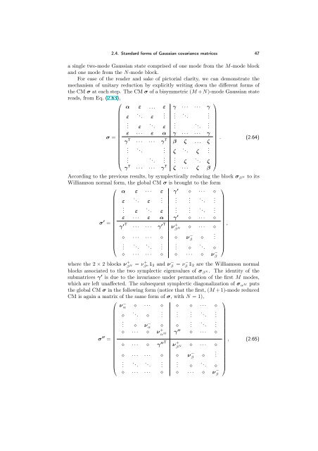
2.4. Standard forms of Gaussian covariance matrices 47 a single two-mode Gaussian state comprised of one mode from the M-mode block and one mode from the N-mode block. For ease of the reader and sake of pictorial clarity, we can demonstrate the mechanism of unitary reduction by explicitly writing down the different forms of the CM σ at each step. The CM σ of a bisymmetric (M +N)-mode Gaussian state reads, from Eq. (2.63), ⎛ α ε . . . ε γ · · · · · · γ ⎜ . ⎜ ε .. . . . ε . . .. . . ⎜ . . ⎜ . ε .. . . ε . .. . . ⎜ ε · · · ε α γ · · · · · · γ σ = ⎜ γ ⎜ ⎝ T · · · · · · γT β ζ . . . ζ . . . .. . . . ζ .. . ζ . . . .. . . . ζ .. ζ γT · · · · · · γT ⎞ ⎟ . (2.64) ⎟ ⎠ ζ · · · ζ β According to the previous results, by symplectically reducing the block σβN to its Williamson normal form, the global CM σ is brought to the form σ ′ ⎛ α ε · · · ε γ ⎜ = ⎜ ⎝ ′ ⋄ · · · ⋄ ε . ε . .. ε · · · ε . .. ε . ε α . . γ . . . .. . .. . . ′ γ ⋄ · · · ⋄ ′T · · · · · · γ ′T + ν βN ⋄ · · · · · · ⋄ ⋄ ⋄ ν · · · ⋄ − ⎞ . . .. . .. . . β ⋄ ⋄ . .. . . ⋄ ⎟ , ⎟ ⎠ ⋄ · · · · · · ⋄ ⋄ · · · ⋄ ν − β where the 2 × 2 blocks ν + βN = ν + βn2 and ν − β = ν− β 2 are the Williamson normal blocks associated to the two symplectic eigenvalues of σ β N . The identity of the submatrices γ ′ is due to the invariance under permutation of the first M modes, which are left unaffected. The subsequent symplectic diagonalization of σ α M puts the global CM σ in the following form (notice that the first, (M + 1)-mode reduced CM is again a matrix of the same form of σ, with N = 1), ⎛ σ ′′ ⎜ = ⎜ ⎝ ν − α ⋄ · · · ⋄ ⋄ ⋄ · · · ⋄ ⋄ . .. ⋄ . . . . . . ⋄ ν− α ⋄ ⋄ . . . . . .. . .. . . . . ⋄ · · · ⋄ ν + α M γ ′′ ⋄ · · · ⋄ ⋄ · · · ⋄ γ ′′T ν + β N ⋄ · · · ⋄ ⋄ · · · · · · ⋄ ⋄ ν − β . . . .. . .. . . . . ⋄ ⋄ . . .. ⋄ ⋄ · · · · · · ⋄ ⋄ · · · ⋄ ν − β ⎞ ⎟ , (2.65) ⎟ ⎠
- Page 10 and 11: x Contents 2.2.2.2. Symplectic repr
- Page 12 and 13: xii Contents 7.2.3. Tripartite enta
- Page 14 and 15: xiv Contents Chapter 13. Entangleme
- Page 17 and 18: Introduction About eighty years aft
- Page 19 and 20: Introduction 5 Gaussian states. Imp
- Page 21: Introduction 7 The companion Part V
- Page 24 and 25: 10 1. Characterizing entanglement a
- Page 26 and 27: 12 1. Characterizing entanglement w
- Page 28 and 29: 14 1. Characterizing entanglement W
- Page 30 and 31: 16 1. Characterizing entanglement F
- Page 32 and 33: 18 1. Characterizing entanglement a
- Page 34 and 35: 20 1. Characterizing entanglement i
- Page 36 and 37: 22 1. Characterizing entanglement e
- Page 38 and 39: 24 1. Characterizing entanglement n
- Page 40 and 41: 26 1. Characterizing entanglement p
- Page 43 and 44: CHAPTER 2 Gaussian states: structur
- Page 45 and 46: 2.1. Introduction to continuous var
- Page 47 and 48: 2.2. Mathematical description of Ga
- Page 49 and 50: 2.2. Mathematical description of Ga
- Page 51 and 52: 2.3. Degree of information encoded
- Page 53 and 54: 2.3. Degree of information encoded
- Page 55 and 56: 2.4. Standard forms of Gaussian cov
- Page 57 and 58: 2.4. Standard forms of Gaussian cov
- Page 59: 2.4. Standard forms of Gaussian cov
- Page 63: Part II Bipartite entanglement of G
- Page 66 and 67: 52 3. Characterizing entanglement o
- Page 68 and 69: 54 3. Characterizing entanglement o
- Page 71 and 72: CHAPTER 4 Two-mode entanglement Thi
- Page 73 and 74: 4.2. Entanglement and symplectic ei
- Page 75 and 76: 4.3. Entanglement versus Entropic m
- Page 77 and 78: 1 0.75 0.5 SL1 0.25 0 (a) 4.3. Enta
- Page 79 and 80: 4.3. Entanglement versus Entropic m
- Page 81 and 82: Μ Μ1Μ2 3 2 1 1 4.3. Entanglemen
- Page 83 and 84: 4.3. Entanglement versus Entropic m
- Page 85 and 86: 4.3. Entanglement versus Entropic m
- Page 87 and 88: global generalized entropy S3 globa
- Page 89 and 90: 4.4. Quantifying entanglement via p
- Page 91 and 92: 4.4. Quantifying entanglement via p
- Page 93 and 94: 4.5. Gaussian entanglement measures
- Page 95 and 96: 4.5. Gaussian entanglement measures
- Page 97 and 98: 4.5. Gaussian entanglement measures
- Page 99 and 100: 4.5. Gaussian entanglement measures
- Page 101 and 102: Ν p Σopt 1 0.8 0.6 0.4 0.2 0 4.5
- Page 103 and 104: GEF GEF 4 3 2 1 0 4.6. Summary and
- Page 105: 4.6. Summary and further remarks 91
- Page 108 and 109: 94 5. Multimode entanglement under
2.4. Standard forms of Gaussian covariance matrices 47<br />
a single two-mode Gaussian state comprised of one mode from the M-mode block<br />
and one mode from the N-mode block.<br />
For ease of the reader and sake of pictorial clarity, we can demonstrate the<br />
mechanism of unitary reduction by explicitly writing down the different forms of<br />
the CM σ at each step. The CM σ of a bisymmetric (M +N)-mode Gaussian state<br />
reads, from Eq. (2.63),<br />
⎛<br />
α ε . . . ε γ · · · · · · γ<br />
⎜<br />
.<br />
⎜ ε ..<br />
. . .<br />
ε . . ..<br />
.<br />
.<br />
⎜<br />
. .<br />
⎜ . ε ..<br />
. .<br />
ε . ..<br />
.<br />
.<br />
⎜ ε · · · ε α γ · · · · · · γ<br />
σ = ⎜<br />
γ<br />
⎜<br />
⎝<br />
T · · · · · · γT β ζ . . . ζ<br />
. .<br />
. ..<br />
. .<br />
. ζ ..<br />
.<br />
ζ .<br />
.<br />
. ..<br />
.<br />
. . ζ .. ζ<br />
γT · · · · · · γT ⎞<br />
⎟ . (2.64)<br />
⎟<br />
⎠<br />
ζ · · · ζ β<br />
According to the previous results, by symplectically reducing the block σβN to its<br />
Williamson normal form, the global CM σ is brought to the form<br />
σ ′ ⎛<br />
α ε · · · ε γ<br />
⎜<br />
= ⎜<br />
⎝<br />
′ ⋄ · · · ⋄<br />
ε<br />
.<br />
ε<br />
. ..<br />
ε<br />
· · ·<br />
ε<br />
. ..<br />
ε<br />
.<br />
ε<br />
α<br />
.<br />
.<br />
γ<br />
.<br />
.<br />
. ..<br />
. ..<br />
.<br />
.<br />
′ γ<br />
⋄ · · · ⋄<br />
′T<br />
· · · · · · γ ′T +<br />
ν βN ⋄ · · · · · · ⋄ ⋄<br />
⋄<br />
ν<br />
· · · ⋄<br />
−<br />
⎞<br />
.<br />
. .. . .. .<br />
.<br />
β<br />
⋄<br />
⋄<br />
. ..<br />
.<br />
.<br />
⋄<br />
⎟ ,<br />
⎟<br />
⎠<br />
⋄ · · · · · · ⋄ ⋄ · · · ⋄ ν −<br />
β<br />
where the 2 × 2 blocks ν +<br />
βN = ν +<br />
βn2 and ν −<br />
β<br />
= ν−<br />
β 2 are the Williamson normal<br />
blocks associated to the two symplectic eigenvalues of σ β N . The identity of the<br />
submatrices γ ′ is due to the invariance under permutation of the first M modes,<br />
which are left unaffected. The subsequent symplectic diagonalization of σ α M puts<br />
the global CM σ in the following form (notice that the first, (M + 1)-mode reduced<br />
CM is again a matrix of the same form of σ, with N = 1),<br />
⎛<br />
σ ′′ ⎜<br />
= ⎜<br />
⎝<br />
ν − α ⋄ · · · ⋄ ⋄ ⋄ · · · ⋄<br />
⋄<br />
. .. ⋄<br />
.<br />
.<br />
.<br />
.<br />
.<br />
. ⋄ ν− α ⋄ ⋄<br />
.<br />
.<br />
.<br />
.<br />
. ..<br />
. ..<br />
.<br />
.<br />
.<br />
.<br />
⋄ · · · ⋄ ν +<br />
α M γ ′′ ⋄ · · · ⋄<br />
⋄ · · · ⋄ γ ′′T ν +<br />
β N ⋄ · · · ⋄<br />
⋄ · · · · · · ⋄ ⋄ ν −<br />
β<br />
. .<br />
. .. . ..<br />
. .<br />
. . ⋄<br />
⋄<br />
.<br />
. .. ⋄<br />
⋄ · · · · · · ⋄ ⋄ · · · ⋄ ν −<br />
β<br />
⎞<br />
⎟ , (2.65)<br />
⎟<br />
⎠


