ENTANGLEMENT OF GAUSSIAN STATES Gerardo Adesso

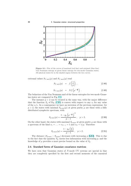
40 2. Gaussian states: structural properties
SV SV
5
4
3
2
1
0
0 0.2 0.4 0.6 0.8 1
SL SL
Figure 2.1. Plot of the curves of maximal (red line) and minimal (blue line)
Von Neumann entropy at given linear entropy for two-mode Gaussian states.
All physical states lie in the shaded region between the two curves.
extremal values SV min(µ) and SV max(µ) read
1
SV min(µ) = f ,
µ
(2.48)
SV max(µ) =
Nf µ − 1
N . (2.49)
The behaviors of the Von Neumann and of the linear entropies for two-mode Gaussian
states are compared in Fig. 2.1.
The instance p > 2 can be treated in the same way, with the major difference
that the function Sp of Eq. (2.41) is convex with respect to any si for any value
of the si’s. As a consequence we have an inversion of the previous expressions: for
p > 2, the states with minimal Sp min(µ) at given purity µ are those with a fully
distributed symplectic spectrum, with
µ − 1
N N
1 − gp
Sp min(µ) =
p − 1
, p > 2 . (2.50)
On the other hand, the states with maximal Sp max at given purity µ are those with
a spectrum of the kind ν1 = . . . = νN−1 = 1 and νN = 1/µ. Therefore
1 1 − gp µ
Sp max(µ) =
, p > 2 .
p − 1
(2.51)
The distance |Sp max − Sp min| decreases with increasing p [GA3]. This is due
to the fact that the quantity Sp carries less information with increasing p, and the
knowledge of µ provides a more precise bound on the value of Sp.
2.4. Standard forms of Gaussian covariance matrices
We have seen that Gaussian states of N-mode CV systems are special in that
they are completely specified by the first and second moments of the canonical