ENTANGLEMENT OF GAUSSIAN STATES Gerardo Adesso
ENTANGLEMENT OF GAUSSIAN STATES Gerardo Adesso ENTANGLEMENT OF GAUSSIAN STATES Gerardo Adesso
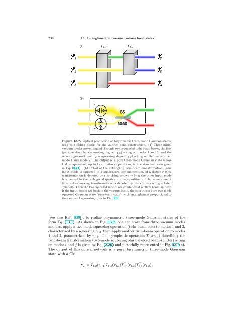
230 13. Entanglement in Gaussian valence bond states γγγγ 0000 1 γγγγ 0000 2 γγγγ 0000 3 (a) (b) r -r r 1,3 50:50 r 1,2 Figure 13.7. Optical production of bisymmetric three-mode Gaussian states, used as building blocks for the valence bond construction. (a) Three initial vacuum modes are entangled through two sequential twin-beam boxes, the first (parametrized by a squeezing degree r1,3) acting on modes 1 and 3, and the second (parametrized by a squeezing degree r1,2) acting on the transformed mode 1 and mode 2. The output is a pure three-mode Gaussian state whose CM is equivalent, up to local unitary operations, to the standard form given in Eq. (13.1). (b) Detail of the entangling twin-beam transformation. One input mode is squeezed in a quadrature, say momentum, of a degree r (this transformation is denoted by stretching arrows →| |←); the other input mode is squeezed in the orthogonal quadrature, say position, of the same amount (this anti-squeezing transformation is denoted by the corresponding rotated symbol). Then the two squeezed modes are combined at a 50:50 beam-splitter. If the input modes are both in the vacuum state, the output is a pure two-mode squeezed Gaussian state (twin-beam state), with entanglement proportional to the degree of squeezing r, as in Fig. 9.1. (see also Ref. [238]), to realize bisymmetric three-mode Gaussian states of the form Eq. (13.1). As shown in Fig. 13.7, one can start from three vacuum modes and first apply a two-mode squeezing operation (twin-beam box) to modes 1 and 3, characterized by a squeezing r1,3, then apply another twin-beam operation to modes 1 and 2, parametrized by r1,2. The symplectic operation Ti,j(ri,j) describing the twin-beam transformation (two-mode squeezing plus balanced beam-splitter) acting on modes i and j is given by Eq. (2.28) and pictorially represented in Fig. 13.7(b). The output of this optical network is a pure, bisymmetric, three-mode Gaussian state with a CM BS γ B = T1,2(r1,2)T1,3(r1,3)T T 1,3(r1,3)T T 1,2(r1,2) , γγγγ s γγγγ s γγγγ x
of the form Eq. (13.1), with 13.3. Optical implementation of Gaussian valence bond states 231 γs = 1 diag 2 e−2r1,2 e 4r1,2 cosh (2r1,3) + 1 , 1 2 e−2r1,2 4r1,2 cosh (2r1,3) + e , γx εss = = diag {cosh (2r1,3) , cosh (2r1,3)}, 1 diag 2 e−2r1,2 e 4r1,2 cosh (2r1,3) − 1 , 1 2 e−2r1,2 εsx = 4r1,2 cosh (2r1,3) − e , √ r1,2 diag 2e cosh (r1,3) sinh (r1,3) , − √ 2e −r1,2 cosh (r1,3) sinh (r1,3) . (13.7) By means of local symplectic operations (unitary on the Hilbert space), like additional single-mode squeezings, the CM γ B can be brought in the standard form of Eq. (13.2), from which one has √ x + 1 r1,3 = arccos √ , 2 √−x 3 + 2x2 + 4s2x − x r1,2 = arccos 4x + 1 2 . (13.8) For a given r1,3 (i.e. at fixed x), the quantity r1,2 is a monotonically increasing function of the standard form covariance s, so this squeezing parameter which enters in the production of the building block (see Fig. 13.7) directly regulates the entanglement distribution in the target GVBS, as discussed in Sec. 13.2. The only unfeasible part of the scheme seems constituted by the ancillary EPR pairs. But are infinitely entangled bonds truly necessary? In Ref. [GA13] we have considered the possibility of using a Γ in given by the direct sum of two-mode squeezed states of Eq. (2.22), but with finite r. Repeating the analysis of Sec. 13.2 to investigate the entanglement properties of the resulting GVBS with finitely entangled bonds, it is found that, at fixed (x, s), the entanglement in the various partitions is degraded as r decreases, as somehow expected. Crucially, this does not affect the connection between input entanglement and output correlation length. Numerical investigations show that, while the thresholds sk for the onset of entanglement between distant pairs are quantitatively modified — namely, a bigger s is required at a given x to compensate the less entangled bonds — the overall structure stays untouched. As an example, Fig. 13.5(b) depicts the entanglement distribution in six-mode GVBS obtained from finitely entangled bonds with r = 1.1, corresponding to ≈ 6.6 dB of squeezing (an achievable value [224]). This ensures that the possibility of engineering the entanglement structure in GVBS via the properties of the building block is robust against imperfect resources, definitely meaning that the presented scheme is feasible. Alternatively, one could from the beginning observe that the triples consisting of two projective measurements and one EPR pair can be replaced by a single projection onto the EPR state, applied at each site i between the input mode 2 of the building block and the consecutive input mode 1 of the building block of site i + 1 [202]. The output of all the homodyne measurements would conditionally realize the target GVBS.
- Page 193 and 194: (out) (in) TRITTER 10.1. Optical pr
- Page 195 and 196: 10.2. How to produce and exploit un
- Page 197 and 198: CHAPTER 11 Efficient production of
- Page 199 and 200: 11.2. Generic entanglement and stat
- Page 201 and 202: 11.2. Generic entanglement and stat
- Page 203 and 204: 11.2. Generic entanglement and stat
- Page 205 and 206: 11.3. Economical state engineering
- Page 207: Part V Operational interpretation a
- Page 210 and 211: 196 12. Multiparty quantum communic
- Page 212 and 213: 198 12. Multiparty quantum communic
- Page 214 and 215: 200 12. Multiparty quantum communic
- Page 216 and 217: 202 12. Multiparty quantum communic
- Page 218 and 219: 204 12. Multiparty quantum communic
- Page 220 and 221: 206 12. Multiparty quantum communic
- Page 222 and 223: 208 12. Multiparty quantum communic
- Page 224 and 225: 210 12. Multiparty quantum communic
- Page 226 and 227: 212 12. Multiparty quantum communic
- Page 228 and 229: 214 12. Multiparty quantum communic
- Page 230 and 231: 216 12. Multiparty quantum communic
- Page 233 and 234: CHAPTER 13 Entanglement in Gaussian
- Page 235 and 236: 13.1. Gaussian valence bond states
- Page 237 and 238: Eq. (13.3) thus takes the form 13.1
- Page 239 and 240: 13.2. Entanglement distribution in
- Page 241 and 242: s 20 17.5 15 12.5 10 7.5 5 2.5 13.2
- Page 243: 13.3. Optical implementation of Gau
- Page 247 and 248: 13.4. Telecloning with Gaussian val
- Page 249 and 250: CHAPTER 14 Gaussian entanglement sh
- Page 251 and 252: 14.1. Entanglement in non-inertial
- Page 253 and 254: 14.2. Distributed Gaussian entangle
- Page 255 and 256: 14.2. Distributed Gaussian entangle
- Page 257 and 258: 14.2. Distributed Gaussian entangle
- Page 259 and 260: 6 s 4 14.2. Distributed Gaussian en
- Page 261 and 262: 2.5 0 0 5 10 IΣAR7.5 0 14.3. Distr
- Page 263 and 264: 14.3. Distributed Gaussian entangle
- Page 265 and 266: 0 entanglement condition 14.3. Dist
- Page 267 and 268: 14.3. Distributed Gaussian entangle
- Page 269 and 270: 14.3. Distributed Gaussian entangle
- Page 271 and 272: 4 3 a 2 1 14.4. Discussion and outl
- Page 273: Part VI Closing remarks Entanglemen
- Page 276 and 277: 262 Conclusion and Outlook Gaussian
- Page 278 and 279: 264 Conclusion and Outlook compass
- Page 280 and 281: 266 A. Standard forms of pure Gauss
- Page 282 and 283: 268 A. Standard forms of pure Gauss
- Page 284 and 285: 270 A. Standard forms of pure Gauss
- Page 286 and 287: 272 List of Publications [GA11] G.
- Page 288 and 289: 274 Bibliography [23] C. H. Bennett
- Page 290 and 291: 276 Bibliography [79] J. Eisert, C.
- Page 292 and 293: 278 Bibliography [140] J. Laurat, T
230 13. Entanglement in Gaussian valence bond states<br />
γγγγ 0000 1<br />
γγγγ 0000 2<br />
γγγγ 0000 3<br />
(a)<br />
(b)<br />
r<br />
-r<br />
r 1,3<br />
50:50<br />
r 1,2<br />
Figure 13.7. Optical production of bisymmetric three-mode Gaussian states,<br />
used as building blocks for the valence bond construction. (a) Three initial<br />
vacuum modes are entangled through two sequential twin-beam boxes, the first<br />
(parametrized by a squeezing degree r1,3) acting on modes 1 and 3, and the<br />
second (parametrized by a squeezing degree r1,2) acting on the transformed<br />
mode 1 and mode 2. The output is a pure three-mode Gaussian state whose<br />
CM is equivalent, up to local unitary operations, to the standard form given<br />
in Eq. (13.1). (b) Detail of the entangling twin-beam transformation. One<br />
input mode is squeezed in a quadrature, say momentum, of a degree r (this<br />
transformation is denoted by stretching arrows →| |←); the other input mode<br />
is squeezed in the orthogonal quadrature, say position, of the same amount<br />
(this anti-squeezing transformation is denoted by the corresponding rotated<br />
symbol). Then the two squeezed modes are combined at a 50:50 beam-splitter.<br />
If the input modes are both in the vacuum state, the output is a pure two-mode<br />
squeezed Gaussian state (twin-beam state), with entanglement proportional to<br />
the degree of squeezing r, as in Fig. 9.1.<br />
(see also Ref. [238]), to realize bisymmetric three-mode Gaussian states of the<br />
form Eq. (13.1). As shown in Fig. 13.7, one can start from three vacuum modes<br />
and first apply a two-mode squeezing operation (twin-beam box) to modes 1 and 3,<br />
characterized by a squeezing r1,3, then apply another twin-beam operation to modes<br />
1 and 2, parametrized by r1,2. The symplectic operation Ti,j(ri,j) describing the<br />
twin-beam transformation (two-mode squeezing plus balanced beam-splitter) acting<br />
on modes i and j is given by Eq. (2.28) and pictorially represented in Fig. 13.7(b).<br />
The output of this optical network is a pure, bisymmetric, three-mode Gaussian<br />
state with a CM<br />
BS<br />
γ B = T1,2(r1,2)T1,3(r1,3)T T 1,3(r1,3)T T 1,2(r1,2) ,<br />
γγγγ s<br />
γγγγ s<br />
γγγγ x


