ENTANGLEMENT OF GAUSSIAN STATES Gerardo Adesso

s
20
17.5
15
12.5
10
7.5
5
2.5
13.2. Entanglement distribution in Gaussian valence bond states 227
50
(a) (b)
long-range entanglement
next-n.n.
nearest neighbors
unphysical
2.5 5 7.5 10 12.5 15 17.5 20
x
s
40
30
20
10
0
long-range entanglement
next-n.n.
nearest neighbors
unphysical
2.5 5 7.5 10 12.5 15 17.5 20
x
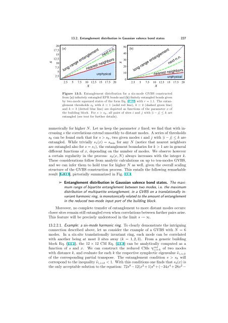
Figure 13.5. Entanglement distribution for a six-mode GVBS constructed
from (a) infinitely entangled EPR bonds and (b) finitely entangled bonds given
by two-mode squeezed states of the form Eq. (2.22) with r = 1.1. The entanglement
thresholds sk with k = 1 (solid red line), k = 2 (dashed green line)
and k = 3 (dotted blue line) are depicted as functions of the parameter x of
the building block. For s > sk, all pairs of sites i and j with |i − j| ≤ k are
entangled (see text for further details).
numerically for higher N. Let us keep the parameter x fixed; we find that with increasing
s the correlations extend smoothly to distant modes. A series of thresholds
sk can be found such that for s > sk, two given modes i and j with |i − j| ≤ k are
entangled. While trivially s1(x) = smin for any N (notice that nearest neighbors
are entangled also for s = s1), the entanglement boundaries for k > 1 are in general
different functions of x, depending on the number of modes. We observe however
a certain regularity in the process: sk(x, N) always increases with the integer k.
These considerations follow from analytic calculations on up to ten-modes GVBS,
and we can infer them to hold true for higher N as well, given the overall scaling
structure of the GVBS construction process. This entails the following remarkable
result [GA13], pictorially summarized in Fig. 13.4.
➢ Entanglement distribution in Gaussian valence bond states. The maximum
range of bipartite entanglement between two modes, i.e. the maximum
distribution of multipartite entanglement, in a GVBS on a translationally invariant
harmonic ring, is monotonically related to the amount of entanglement
in the reduced two-mode input port of the building block.
Moreover, no complete transfer of entanglement to more distant modes occurs:
closer sites remain still entangled even when correlations between farther pairs arise.
This feature will be precisely understood in the limit s → ∞.
13.2.2.1. Example: a six-mode harmonic ring. To clearly demonstrate the intriguing
connection described above, let us consider the example of a GVBS with N = 6
modes. In a six-site translationally invariant ring, each mode can be correlated
with another being at most 3 sites away (k = 1, 2, 3). From a generic building
block Eq. (13.1), the 12 × 12 CM Eq. (13.3) can be analytically computed as a
function of s and x. We can construct the reduced CMs γout i,i+k of two modes
with distance k, and evaluate for each k the respective symplectic eigenvalue ˜νi,i+k
of the corresponding partial transpose. The entanglement condition s > sk will
correspond to the inequality ˜νi,i+k < 1. With this conditions one finds that s2(x) is
the only acceptable solution to the equation: 72s8 −12(x2 +1)s6 +(−34x4 +28x2 −