ENTANGLEMENT OF GAUSSIAN STATES Gerardo Adesso
ENTANGLEMENT OF GAUSSIAN STATES Gerardo Adesso ENTANGLEMENT OF GAUSSIAN STATES Gerardo Adesso
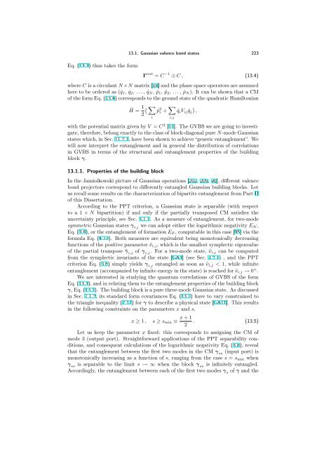
222 13. Entanglement in Gaussian valence bond states (1) (2) (3) (4) Alice 0 1 2 Bob Alice 0 1 2 Bob Alice 0 1 2 Bob Alice 0 1 2 Bob (9) Figure 13.2. How a Gaussian valence bond state is created via continuousvariable entanglement swapping. At each step, Alice attempts to teleport her mode 0 (half of an EPR bond, depicted in yellow) to Bob, exploiting as an entangled resource two of the three modes of the building block (denoted at each step by 1 and 2). The curly bracket denotes homodyne detection, which together with classical communication and conditional displacement at Bob’s side achieves teleportation. The state will be approximately recovered in mode 2, owned by Bob. Since mode 0, at each step, is entangled with the respective half of an EPR bond, the process swaps entanglement from the ancillary chain of the EPR bonds to the modes in the building block. The picture has to be followed column-wise. For ease of clarity, we depict the process as constituted by two sequences: in the first sequence [frames (1) to (4)] modes 1 and 2 are the two input modes of the building block (depicted in blue); in the second sequence [frames (5) to (8)] modes 1 and 2 are respectively an input and an output mode of the building block. As a result of the multiple entanglement swapping [frame (9)] the chain of the output modes (depicted in red), initially in a product state, is transformed into a translationally invariant Gaussian valence bond state, possessing in general multipartite entanglement among all the modes (depicted in magenta). to the physical one, will affect the structure and entanglement properties of the target GVBS. This link is explored in the following Section. We note here that the Gaussian states generally constructed according to the above procedure are ground states of harmonic Hamiltonians (a property of all GVBS [202]). This follows as no mutual correlations are ever created between the operators ˆqi and ˆpj for any i, j = 1, . . . , N, due to the fact that both EPR bonds and building blocks are chosen from the beginning in standard form. The final CM 2 Bob Alice 0 1 2 Bob Alice 0 1 2 Bob Alice 0 1 2 Bob Alice 0 1 (5) (6) (7) (8)
Eq. (13.3) thus takes the form 13.1. Gaussian valence bond states 223 Γ out = C −1 ⊕ C , (13.4) where C is a circulant N ×N matrix [18] and the phase space operators are assumed here to be ordered as (ˆq1, ˆq2, . . . , ˆqN, ˆp1, ˆp2, . . . , ˆpN). It can be shown that a CM of the form Eq. (13.4) corresponds to the ground state of the quadratic Hamiltonian ˆH = 1 2 i ˆp 2 i + i,j ˆqiVij ˆqj , with the potential matrix given by V = C 2 [11]. The GVBS we are going to investigate, therefore, belong exactly to the class of block-diagonal pure N-mode Gaussian states which, in Sec. 11.2.1, have been shown to achieve “generic entanglement”. We will now interpret the entanglement and in general the distribution of correlations in GVBS in terms of the structural and entanglement properties of the building block γ. 13.1.1. Properties of the building block In the Jamiolkowski picture of Gaussian operations [202, 205, 90], different valence bond projectors correspond to differently entangled Gaussian building blocks. Let us recall some results on the characterization of bipartite entanglement from Part II of this Dissertation. According to the PPT criterion, a Gaussian state is separable (with respect to a 1 × N bipartition) if and only if the partially transposed CM satisfies the uncertainty principle, see Sec. 3.1.1. As a measure of entanglement, for two-mode symmetric Gaussian states γ i,j we can adopt either the logarithmic negativity EN , Eq. (3.8), or the entanglement of formation EF , computable in this case [95] via the formula Eq. (4.17). Both measures are equivalent being monotonically decreasing functions of the positive parameter ˜νi,j, which is the smallest symplectic eigenvalue of the partial transpose ˜γ i,j of γ i,j. For a two-mode state, ˜νi,j can be computed from the symplectic invariants of the state [GA3] (see Sec. 4.2.1) , and the PPT criterion Eq. (3.6) simply yields γ i,j entangled as soon as ˜νi,j < 1, while infinite entanglement (accompanied by infinite energy in the state) is reached for ˜νi,j → 0 + . We are interested in studying the quantum correlations of GVBS of the form Eq. (13.3), and in relating them to the entanglement properties of the building block γ, Eq. (13.1). The building block is a pure three-mode Gaussian state. As discussed in Sec. 7.1.2, its standard form covariances Eq. (13.2) have to vary constrained to the triangle inequality (7.17) for γ to describe a physical state [GA11]. This results in the following constraints on the parameters x and s, x + 1 x ≥ 1 , s ≥ smin ≡ . (13.5) 2 Let us keep the parameter x fixed: this corresponds to assigning the CM of mode 3 (output port). Straightforward applications of the PPT separability conditions, and consequent calculations of the logarithmic negativity Eq. (3.8), reveal that the entanglement between the first two modes in the CM γss (input port) is monotonically increasing as a function of s, ranging from the case s = smin when γss is separable to the limit s → ∞ when the block γss is infinitely entangled. Accordingly, the entanglement between each of the first two modes γs of γ and the
- Page 186 and 187: 172 9. Two-mode Gaussian states in
- Page 189 and 190: CHAPTER 10 Tripartite and four-part
- Page 191 and 192: 10.1. Optical production of three-m
- Page 193 and 194: (out) (in) TRITTER 10.1. Optical pr
- Page 195 and 196: 10.2. How to produce and exploit un
- Page 197 and 198: CHAPTER 11 Efficient production of
- Page 199 and 200: 11.2. Generic entanglement and stat
- Page 201 and 202: 11.2. Generic entanglement and stat
- Page 203 and 204: 11.2. Generic entanglement and stat
- Page 205 and 206: 11.3. Economical state engineering
- Page 207: Part V Operational interpretation a
- Page 210 and 211: 196 12. Multiparty quantum communic
- Page 212 and 213: 198 12. Multiparty quantum communic
- Page 214 and 215: 200 12. Multiparty quantum communic
- Page 216 and 217: 202 12. Multiparty quantum communic
- Page 218 and 219: 204 12. Multiparty quantum communic
- Page 220 and 221: 206 12. Multiparty quantum communic
- Page 222 and 223: 208 12. Multiparty quantum communic
- Page 224 and 225: 210 12. Multiparty quantum communic
- Page 226 and 227: 212 12. Multiparty quantum communic
- Page 228 and 229: 214 12. Multiparty quantum communic
- Page 230 and 231: 216 12. Multiparty quantum communic
- Page 233 and 234: CHAPTER 13 Entanglement in Gaussian
- Page 235: 13.1. Gaussian valence bond states
- Page 239 and 240: 13.2. Entanglement distribution in
- Page 241 and 242: s 20 17.5 15 12.5 10 7.5 5 2.5 13.2
- Page 243 and 244: 13.3. Optical implementation of Gau
- Page 245 and 246: of the form Eq. (13.1), with 13.3.
- Page 247 and 248: 13.4. Telecloning with Gaussian val
- Page 249 and 250: CHAPTER 14 Gaussian entanglement sh
- Page 251 and 252: 14.1. Entanglement in non-inertial
- Page 253 and 254: 14.2. Distributed Gaussian entangle
- Page 255 and 256: 14.2. Distributed Gaussian entangle
- Page 257 and 258: 14.2. Distributed Gaussian entangle
- Page 259 and 260: 6 s 4 14.2. Distributed Gaussian en
- Page 261 and 262: 2.5 0 0 5 10 IΣAR7.5 0 14.3. Distr
- Page 263 and 264: 14.3. Distributed Gaussian entangle
- Page 265 and 266: 0 entanglement condition 14.3. Dist
- Page 267 and 268: 14.3. Distributed Gaussian entangle
- Page 269 and 270: 14.3. Distributed Gaussian entangle
- Page 271 and 272: 4 3 a 2 1 14.4. Discussion and outl
- Page 273: Part VI Closing remarks Entanglemen
- Page 276 and 277: 262 Conclusion and Outlook Gaussian
- Page 278 and 279: 264 Conclusion and Outlook compass
- Page 280 and 281: 266 A. Standard forms of pure Gauss
- Page 282 and 283: 268 A. Standard forms of pure Gauss
- Page 284 and 285: 270 A. Standard forms of pure Gauss
Eq. (13.3) thus takes the form<br />
13.1. Gaussian valence bond states 223<br />
Γ out = C −1 ⊕ C , (13.4)<br />
where C is a circulant N ×N matrix [18] and the phase space operators are assumed<br />
here to be ordered as (ˆq1, ˆq2, . . . , ˆqN, ˆp1, ˆp2, . . . , ˆpN). It can be shown that a CM<br />
of the form Eq. (13.4) corresponds to the ground state of the quadratic Hamiltonian<br />
ˆH = 1<br />
<br />
2<br />
i<br />
ˆp 2 i + <br />
i,j<br />
<br />
ˆqiVij ˆqj ,<br />
with the potential matrix given by V = C 2 [11]. The GVBS we are going to investigate,<br />
therefore, belong exactly to the class of block-diagonal pure N-mode Gaussian<br />
states which, in Sec. 11.2.1, have been shown to achieve “generic entanglement”. We<br />
will now interpret the entanglement and in general the distribution of correlations<br />
in GVBS in terms of the structural and entanglement properties of the building<br />
block γ.<br />
13.1.1. Properties of the building block<br />
In the Jamiolkowski picture of Gaussian operations [202, 205, 90], different valence<br />
bond projectors correspond to differently entangled Gaussian building blocks. Let<br />
us recall some results on the characterization of bipartite entanglement from Part II<br />
of this Dissertation.<br />
According to the PPT criterion, a Gaussian state is separable (with respect<br />
to a 1 × N bipartition) if and only if the partially transposed CM satisfies the<br />
uncertainty principle, see Sec. 3.1.1. As a measure of entanglement, for two-mode<br />
symmetric Gaussian states γ i,j we can adopt either the logarithmic negativity EN ,<br />
Eq. (3.8), or the entanglement of formation EF , computable in this case [95] via the<br />
formula Eq. (4.17). Both measures are equivalent being monotonically decreasing<br />
functions of the positive parameter ˜νi,j, which is the smallest symplectic eigenvalue<br />
of the partial transpose ˜γ i,j of γ i,j. For a two-mode state, ˜νi,j can be computed<br />
from the symplectic invariants of the state [GA3] (see Sec. 4.2.1) , and the PPT<br />
criterion Eq. (3.6) simply yields γ i,j entangled as soon as ˜νi,j < 1, while infinite<br />
entanglement (accompanied by infinite energy in the state) is reached for ˜νi,j → 0 + .<br />
We are interested in studying the quantum correlations of GVBS of the form<br />
Eq. (13.3), and in relating them to the entanglement properties of the building block<br />
γ, Eq. (13.1). The building block is a pure three-mode Gaussian state. As discussed<br />
in Sec. 7.1.2, its standard form covariances Eq. (13.2) have to vary constrained to<br />
the triangle inequality (7.17) for γ to describe a physical state [GA11]. This results<br />
in the following constraints on the parameters x and s,<br />
x + 1<br />
x ≥ 1 , s ≥ smin ≡ . (13.5)<br />
2<br />
Let us keep the parameter x fixed: this corresponds to assigning the CM of<br />
mode 3 (output port). Straightforward applications of the PPT separability conditions,<br />
and consequent calculations of the logarithmic negativity Eq. (3.8), reveal<br />
that the entanglement between the first two modes in the CM γss (input port) is<br />
monotonically increasing as a function of s, ranging from the case s = smin when<br />
γss is separable to the limit s → ∞ when the block γss is infinitely entangled.<br />
Accordingly, the entanglement between each of the first two modes γs of γ and the


