ENTANGLEMENT OF GAUSSIAN STATES Gerardo Adesso
ENTANGLEMENT OF GAUSSIAN STATES Gerardo Adesso ENTANGLEMENT OF GAUSSIAN STATES Gerardo Adesso
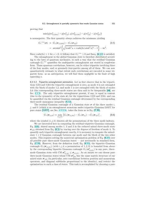
150 8. Unlimited promiscuity of multipartite Gaussian entanglement σσσσ 4a 2 4s 2 4a 2 Figure 8.1. Bipartite entanglement structure in the four-mode Gaussian states σ of Eq. (8.1). The block of modes 1,2 shares with the block of modes 3,4 all the entanglement created originally between modes 2 and 3, which is an increasing function of s (blue springs). Moreover, modes 1 and 2 internally share an entanglement arbitrarily increasing as a function of a, and the same holds for modes 3 and 4 (pink springs). For a approaching infinity, each of the two pairs of modes 1,2 and 3,4 reproduces the entanglement content of an ideal EPR state, while being the same pairs arbitrarily entangled with each other according to value of s. The four-mode state σ reproduces therefore (in the regime of very high a) the entanglement content of two EPR-like pairs ({1, 2} and {3, 4}). Remarkably, there is an additional, independent entanglement between the two pairs, given by Gτ (σ (12)|(34)) = 4s 2 — the original entanglement in the two-mode squeezed state S2,3(s)S T 2,3(s) after the first construction step — which can be itself increased arbitrarily with increasing s. This peculiar distribution of bipartite entanglement, pictorially displayed in Fig. 8.1, is a first remarkable signature of an unmatched freedom of entanglement sharing in multimode Gaussian states as opposed for instance to states of the same number of qubits, where a similar situation is impossible. Specifically, if in a pure state of four qubits the first two approach unit entanglement and the same holds for the last two, the only compatible global state reduces necessarily to a product state of the two singlets: no interpair entanglement is allowed by the fundamental monogamy constraint [59, 169] 8.2.3. Distributed entanglement and multipartite sharing structure We can now move to a closer analysis of entanglement distribution and genuine multipartite quantum correlations. 8.2.3.1. Monogamy inequality. A primary step is to verify whether the fundamental monogamy inequality (6.17) is satisfied on the four-mode state σ distributed among the four parties (each one owning a single mode). 23 In fact, the problem reduces to 23 In Sec. 6.2.3 the general monogamy inequality for N-mode Gaussian states has been established by using the Gaussian tangle, Eq. (6.16). No complete proof is available to date for the monogamy of the (Gaussian) contangle, Eq. (6.13), beyond the tripartite case. Therefore, we need to check its validity explicitly on the state under consideration. 1 2 3 4
proving that 8.2. Entanglement in partially symmetric four-mode Gaussian states 151 min{g[m 2 1|(234) ] − g[m2 1|2 ], g[m2 2|(134) ] − g[m2 1|2 ] − g[m2 2|3 ]} is nonnegative. The first quantity always achieves the minimum yielding Gτ res (σ) ≡ Gτ (σ1|(234)) − Gτ (σ1|2) (8.5) = arcsinh 2 [cosh 2 a + cosh(2s) sinh 2 a] 2 − 1 − 4a 2 . Since cosh(2s) > 1 for s > 0, it follows that Gτ res > 0 and Ineq. (6.17) is satisfied. The entanglement in the global Gaussian state is therefore distributed according to the laws of quantum mechanics, in such a way that the residual Gaussian contangle Gτ res quantifies the multipartite entanglement not stored in couplewise form. Those quantum correlations, however, can be either tripartite involving three of the four modes, and/or genuinely four-partite among all of them. We can now quantitatively estimate to what extent such correlations are encoded in some tripartite form: as an anticipation, we will find them negligible in the limit of high squeezing a. 8.2.3.2. Tripartite entanglement estimation. Let us first observe that in the tripartitions 1|2|4 and 1|3|4 the tripartite entanglement is zero, as mode 4 is not entangled with the block of modes 1,2, and mode 1 is not entangled with the block of modes 3,4 (the corresponding three-mode states are then said to be biseparable [94], see Sec. 7.1.1). The only tripartite entanglement present, if any, is equal in content (due to the symmetry of the state σ) for the tripartitions 1|2|3 and 2|3|4, and can be quantified via the residual Gaussian contangle determined by the corresponding three-mode monogamy inequality (6.17). The residual Gaussian contangle of a Gaussian state σ of the three modes i, j, and k (which is an entanglement monotone under tripartite Gaussian LOCC for pure states [GA10], see Sec. 7.2.2.1), takes the form as in Eq. (7.36), Gτ (σ i|j|k) ≡ min (i,j,k) Gτ (σ i|(jk)) − Gτ (σ i|j) − Gτ (σ i|k) , (8.6) where the symbol (i, j, k) denotes all the permutations of the three mode indexes. We are interested here in computing the residual tripartite Gaussian contangle, Eq. (8.6), shared among modes 1, 2 and 3 in the reduced mixed three-mode state σ123 obtained from Eq. (8.1) by tracing over the degrees of freedom of mode 4. To quantify such tripartite entanglement exactly, it is necessary to compute the mixedstate 1 × 2 Gaussian contangle between one mode and the block of the two other modes. This requires solving the nontrivial optimization problem of Eq. (6.13) over all possible pure three-mode Gaussian states — not necessarily in standard form, Eq. (7.19). However, from the definition itself, Eq. (6.13), the bipartite Gaussian contangle Gτ (σi|(jk)) (with i, j, k a permutation of 1, 2, 3) is bounded from above by the corresponding bipartite Gaussian contangle Gτ (σ p i|(jk) ) in any pure, threemode Gaussian state with CM σ p i|(jk) ≤ σi|(jk). As an ansatz we can choose pure three-mode Gaussian states whose CM σ p 123 has the same matrix structure of our mixed state σ123 (in particular, zero correlations between position and momentum operators, and diagonal subblocks proportional to the identity), and restrict the optimization to such a class of states. This task is accomplished by choosing a pure
- Page 114 and 115: 100 5. Multimode entanglement under
- Page 116 and 117: 102 5. Multimode entanglement under
- Page 118 and 119: 104 5. Multimode entanglement under
- Page 121: Part III Multipartite entanglement
- Page 124 and 125: 110 6. Gaussian entanglement sharin
- Page 126 and 127: 112 6. Gaussian entanglement sharin
- Page 128 and 129: 114 6. Gaussian entanglement sharin
- Page 130 and 131: 116 6. Gaussian entanglement sharin
- Page 132 and 133: 118 6. Gaussian entanglement sharin
- Page 134 and 135: 120 6. Gaussian entanglement sharin
- Page 136 and 137: 122 7. Tripartite entanglement in t
- Page 138 and 139: 124 7. Tripartite entanglement in t
- Page 140 and 141: 126 7. Tripartite entanglement in t
- Page 142 and 143: 128 7. Tripartite entanglement in t
- Page 144 and 145: 130 7. Tripartite entanglement in t
- Page 146 and 147: 132 7. Tripartite entanglement in t
- Page 148 and 149: 134 7. Tripartite entanglement in t
- Page 150 and 151: 136 7. Tripartite entanglement in t
- Page 152 and 153: 138 7. Tripartite entanglement in t
- Page 154 and 155: 140 7. Tripartite entanglement in t
- Page 156 and 157: 142 7. Tripartite entanglement in t
- Page 158 and 159: 144 7. Tripartite entanglement in t
- Page 160 and 161: 146 7. Tripartite entanglement in t
- Page 162 and 163: 148 8. Unlimited promiscuity of mul
- Page 166 and 167: 152 8. Unlimited promiscuity of mul
- Page 168 and 169: 154 8. Unlimited promiscuity of mul
- Page 171: Part IV Quantum state engineering o
- Page 174 and 175: 160 9. Two-mode Gaussian states in
- Page 176 and 177: 162 9. Two-mode Gaussian states in
- Page 178 and 179: 164 9. Two-mode Gaussian states in
- Page 180 and 181: 166 9. Two-mode Gaussian states in
- Page 182 and 183: 168 9. Two-mode Gaussian states in
- Page 184 and 185: 170 9. Two-mode Gaussian states in
- Page 186 and 187: 172 9. Two-mode Gaussian states in
- Page 189 and 190: CHAPTER 10 Tripartite and four-part
- Page 191 and 192: 10.1. Optical production of three-m
- Page 193 and 194: (out) (in) TRITTER 10.1. Optical pr
- Page 195 and 196: 10.2. How to produce and exploit un
- Page 197 and 198: CHAPTER 11 Efficient production of
- Page 199 and 200: 11.2. Generic entanglement and stat
- Page 201 and 202: 11.2. Generic entanglement and stat
- Page 203 and 204: 11.2. Generic entanglement and stat
- Page 205 and 206: 11.3. Economical state engineering
- Page 207: Part V Operational interpretation a
- Page 210 and 211: 196 12. Multiparty quantum communic
- Page 212 and 213: 198 12. Multiparty quantum communic
proving that<br />
8.2. Entanglement in partially symmetric four-mode Gaussian states 151<br />
min{g[m 2 1|(234) ] − g[m2 1|2 ], g[m2 2|(134) ] − g[m2 1|2 ] − g[m2 2|3 ]}<br />
is nonnegative. The first quantity always achieves the minimum yielding<br />
Gτ res (σ) ≡ Gτ (σ1|(234)) − Gτ (σ1|2) (8.5)<br />
= arcsinh 2<br />
<br />
[cosh 2 a + cosh(2s) sinh 2 a] 2 <br />
− 1 − 4a 2 .<br />
Since cosh(2s) > 1 for s > 0, it follows that Gτ res > 0 and Ineq. (6.17) is satisfied.<br />
The entanglement in the global Gaussian state is therefore distributed according<br />
to the laws of quantum mechanics, in such a way that the residual Gaussian<br />
contangle Gτ res quantifies the multipartite entanglement not stored in couplewise<br />
form. Those quantum correlations, however, can be either tripartite involving three<br />
of the four modes, and/or genuinely four-partite among all of them. We can now<br />
quantitatively estimate to what extent such correlations are encoded in some tripartite<br />
form: as an anticipation, we will find them negligible in the limit of high<br />
squeezing a.<br />
8.2.3.2. Tripartite entanglement estimation. Let us first observe that in the tripartitions<br />
1|2|4 and 1|3|4 the tripartite entanglement is zero, as mode 4 is not entangled<br />
with the block of modes 1,2, and mode 1 is not entangled with the block of modes<br />
3,4 (the corresponding three-mode states are then said to be biseparable [94], see<br />
Sec. 7.1.1). The only tripartite entanglement present, if any, is equal in content<br />
(due to the symmetry of the state σ) for the tripartitions 1|2|3 and 2|3|4, and can<br />
be quantified via the residual Gaussian contangle determined by the corresponding<br />
three-mode monogamy inequality (6.17).<br />
The residual Gaussian contangle of a Gaussian state σ of the three modes i,<br />
j, and k (which is an entanglement monotone under tripartite Gaussian LOCC for<br />
pure states [GA10], see Sec. 7.2.2.1), takes the form as in Eq. (7.36),<br />
Gτ (σ i|j|k) ≡ min<br />
(i,j,k)<br />
Gτ (σ i|(jk)) − Gτ (σ i|j) − Gτ (σ i|k) , (8.6)<br />
where the symbol (i, j, k) denotes all the permutations of the three mode indexes.<br />
We are interested here in computing the residual tripartite Gaussian contangle,<br />
Eq. (8.6), shared among modes 1, 2 and 3 in the reduced mixed three-mode state<br />
σ123 obtained from Eq. (8.1) by tracing over the degrees of freedom of mode 4. To<br />
quantify such tripartite entanglement exactly, it is necessary to compute the mixedstate<br />
1 × 2 Gaussian contangle between one mode and the block of the two other<br />
modes. This requires solving the nontrivial optimization problem of Eq. (6.13) over<br />
all possible pure three-mode Gaussian states — not necessarily in standard form,<br />
Eq. (7.19). However, from the definition itself, Eq. (6.13), the bipartite Gaussian<br />
contangle Gτ (σi|(jk)) (with i, j, k a permutation of 1, 2, 3) is bounded from above<br />
by the corresponding bipartite Gaussian contangle Gτ (σ p<br />
i|(jk) ) in any pure, threemode<br />
Gaussian state with CM σ p<br />
i|(jk) ≤ σi|(jk). As an ansatz we can choose pure<br />
three-mode Gaussian states whose CM σ p<br />
123 has the same matrix structure of our<br />
mixed state σ123 (in particular, zero correlations between position and momentum<br />
operators, and diagonal subblocks proportional to the identity), and restrict the<br />
optimization to such a class of states. This task is accomplished by choosing a pure


